Jscatter’s documentation
The aim of Jscatter is treatment of experimental data and models:
Reading and analyzing experimental data with associated attributes as temperature, wavevector, comment, ….
Multidimensional fitting taking attributes into account.
Providing useful models for neutron and X-ray scattering form factors, structure factors and dynamic models (quasi elastic neutron scattering) and other topics.
Simplified plotting with paper ready quality.
Easy model building for non programmers.
Python scripts/Jupyter Notebooks to document data evaluation and modelling.







Main concept
Data are organised in
dataArray/dataListwith attributes as .temperature, .wavevector, .pressure and methods for filter, merging and more. See What are dataArray/dataList.Multidimensional, attribute dependent fitting (least square Levenberg-Marquardt, Bayesian fit, differential evolution, …). See Fitting experimental data or
fit().Provide relative simple plotting commands to allow a fast view on data and possible later pretty up. See Plotting in XmGrace or mpl for an interface to matplotlib.
User write models using the existing model library or self created models. See How to build simple models and How to build a more complex model.
The model library contains routines e.g. for vectorized quadrature (formel) or specialised models for scattering as formfactor (ff), structurefactor (sf), dynamic and Biomacromolecules (bio).
Exemplary functions:
Physical equations and useful formulas as quadrature of vector functions
scatteringLengthDensityCalc()-> Electron density, coh and inc neutron scattering length, mass.
smear()-> Smearing enabling simultaneous fits of differently smeared SANS/SAXS data.
desmear()-> Desmearing according to the Lake algorithm for the above.See formel and smallanglescattering (sas)
Particle Formfactors
ringPolymer()-> General formfactor of a polymer ring.
alternatingCoPolymer()-> Alternating linear copolymer between collapsed and swollen states
multiShellSphere()-> Formfactor of multi shell spherical particles.
multiShellCylinder()-> Formfactor of multi shell cylinder particles with caps.
orientedCloudScattering()-> 2D scattering of an oriented cloud of scatterers.See formfactor (ff)
Particle Structurefactors
RMSA()-> Rescaled MSA structure factor for dilute charged colloidal dispersions.
twoYukawa()-> Structure factor for a two Yukawa potential in mean spherical approximation.
OrnsteinZernikeSolver-> Numerical Solution of the Ornstein-Zernike Equation for user-defined potentials
hydrodynamicFunct()-> Hydrodynamic function from hydrodynamic pair interaction.Dynamics
finiteZimm()-> Zimm model with internal friction -> intermediate scattering function.
diffusionHarmonicPotential()-> Diffusion in harmonic potential-> intermediate scattering function.
methylRotation()-> Incoherent intermediate scattering function of CH3 methyl rotation.
multiArmStarORZ()-> Intermediate scattering function of star polymer.
doubleStretchedExp_w()-> Two stretched exponentials with elastic contribution and resolution smearing.
threeLorentz_w()-> Three Lorents functions with elastic contribution and resolution smearing.See dynamic
biomacromoleules
scatIntUniv()-> Neutron/Xray scattering of protein/DNA with contrast to solvent.
intScatFuncYlm()-> Diffusional dynamics of protein/DNA with contrast to solvent.
diffusionTRUnivTensor()-> Effective diffusion from 6x6 diffusion tensor.
intScatFuncOU()-> ISF I(q,t) for Ornstein-Uhlenbeck process of normal mode domain motions.
For help with an AI coding assistant such as Codex, see Using AI assistants for Jscatter analysis for a simple prompt and project setup.
- How to use Jscatter
see Examples and Beginners Guide / Help or try Jscatter live at
.
# import jscatter and numpy
import numpy as np
import jscatter as js

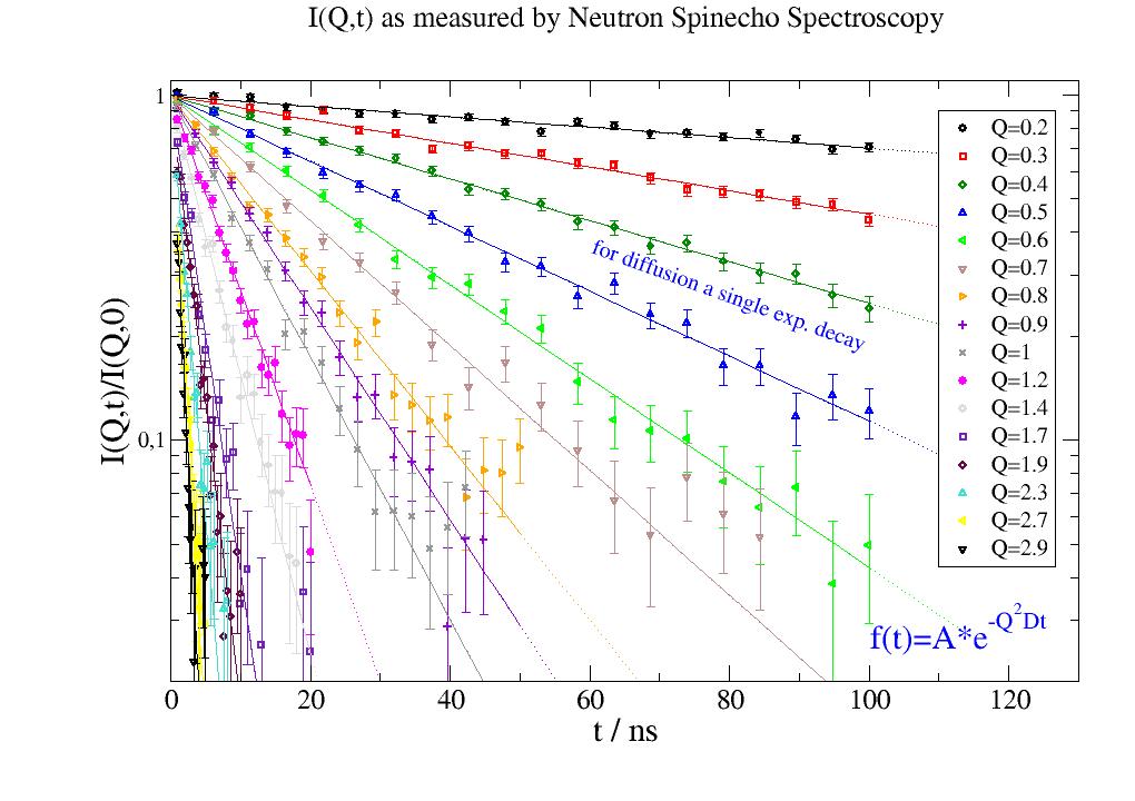
# read the data (16 dataArrays) with attributes as q, Dtrans .... into dataList
i5 = js.dL(js.examples.datapath + '/iqt_1hho.dat')

# define a model for the fit
diffusion = lambda A, D, t, wavevector, e=0: A*np.exp(-wavevector**2*D*t) + e

# do the fit
# single valued start parameters are the same for all 16 dataArrays
# list start parameters [...] indicate independent fitting for dataArrays
# the command line shows progress and the final result, which is found in i5.lastfit
i5.fit(model=diffusion,                         # the fit function
       freepar={'D': [0.08], 'A': 0.98},        # free start parameters
       fixpar={'e': 0.0},                       # fixed parameters
       mapNames={'t': 'X', 'wavevector': 'q'})  # map names from model to data

# open plot with results and residuals
i5.showlastErrPlot(yscale='l')

# open a plot with fixed size and plot data and fit result
p = js.grace(1.2, 0.8)
# plot the data with Q values in legend as symbols
p.plot(i5, symbol=[-1, 0.4, -1], legend='Q=$q')
# plot fit results in lastfit as lines without symbol or legend
p.plot(i5.lastfit, symbol=0, line=[1, 1, -1])
# extend to longer times by changing a model parameter (points)
p.plot(i5.modelValues(t=np.r_[10:120:5]), symbol=0, line=[2, 1, -1])

# pretty up if needed
p.yaxis(min=0.02, max=1.1, scale='log', charsize=1.5, label='I(Q,t)/I(Q,0)')
p.xaxis(min=0, max=130, charsize=1.5, label='t / ns')
p.legend(x=110, y=0.9, charsize=1)
p.title('I(Q,t) as measured by Neutron Spinecho Spectroscopy', size=1.3)
p.text('for diffusion a single exp. decay', x=60, y=0.35, rot=360 - 20, color=4)
p.text(r'f(t)=A*e\S-Q\S2\N\SDt', x=100, y=0.025, rot=0, charsize=1.5)
Shortcuts:
import jscatter as js
js.showDoc()                  # Show html documentation in browser
exampledA=js.dA('test.dat')   # shortcut to create dataArray from file
exampledL=js.dL('test.dat')   # shortcut to create dataList from file
p=js.grace()                  # create plot in XmGrace
p=js.mplot()                  # create plot in matplotlib
p.plot(exampledL)             # plot the read dataList
|
Switch between using mpl and grace in dataArray/dataList fitting. |
|
Switch to headless mode (NO-GUI) to work on a cluster. |
|
Jscatter version is changed in pyproject.toml |
Jscatter package contents
- 1. Beginners Guide / Help
- 1.1. What are dataArray/dataList
- 1.2. First basic examples
- 1.3. Reading ASCII files
- 1.4. Creating from numpy arrays
- 1.5. Manipulating dataArray/dataList
- 1.6. Indexing dataArray/dataList and reducing
- 1.7. Fitting experimental data
- 1.8. Why Fits may fail
- 1.9. Plot experimental data and fit result
- 1.10. Save data and fit results
- 1.11. Additional stuff
- 1.12. Using AI assistants for Jscatter analysis
- 2. dataArray
- 3. dataList
- 4. formel
- 5. smallanglescattering (sas)
- 6. formfactor (ff)
- 7. structurefactor (sf)
- 8. dynamic
- 9. biomacromolecules (bio)
- 10. dls
- 11. Plotting
- 12. Examples
- 13. Intention/Extending
- 14. Installation
- 15. Citing Jscatter
- 16. Changelog