Biomacromolecules (bio)
Examples using the biomacromolecule module (bio) for protein and DNA scattering.
Load PDB structure and calc scattering
Load pdb protein structure from the PDB data bank by ID to scatteringUniverse. The pdb file is corrected and hydrogen is added automatically. The protein structure including H is saved to 3rn3_h.pdb.
import jscatter as js
import numpy as np
uni = js.bio.scatteringUniverse('3rn3')
uni.view()
uni.setSolvent('1d2o1')
uni.qlist = js.loglist(0.1, 5, 100)
# calc scattering both here in D2O
S = js.bio.nscatIntUniv(uni.select_atoms('protein'))
S = js.bio.xscatIntUniv(uni.select_atoms('protein'))
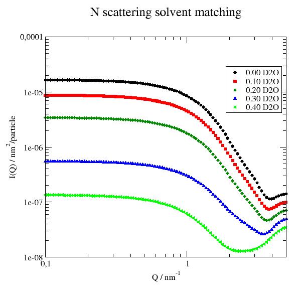
p = js.grace()
p.title('N scattering solvent matching')
p.yaxis(scale='l', label=r'I(Q) / nm\S2\N/particle')
p.xaxis(scale='l', label='Q / nm\S-1')
for x in np.r_[0:0.5:0.1]:
uni.setSolvent([f'{x:.2f}d2o1',f'{1-x:.2f}h2o1' ])
Sn = js.bio.nscatIntUniv(uni.select_atoms('protein'))
p.plot(Sn, le=f'{x:.2f} D2O')
p.legend()
# p.save(js.examples.imagepath+'/biosolventmatching.jpg', size=(2, 2))
Protein scattering and effective diffusion
Protein scattering for different molecular weight proteins at 10 g/l concentration.
We assume here rigid protein structures without internal fluctuations. The diffusion corresponds accordingly to the rigid body diffusion of a protein.
See Exploring internal protein dynamics by neutron spin echo spectroscopy for details.
import jscatter as js
import numpy as np
import scipy.constants as constants
adh = js.bio.fetch_pdb('4w6z.pdb1')
# the 2 dimers in are in model 1 and 2 and need to be merged into one.
adhmerged = js.bio.mergePDBModel(adh)
p = js.grace(1.4, 1)
p.multi(1, 2)
for cc, pdb in enumerate(['3rn3', '3pgk', adhmerged], 1):
# create universe; M and Z are for wrong named Mg and Zn in the pdb files
uni = js.bio.scatteringUniverse(pdb, vdwradii={'M': 1.73, 'Z': 1.7})
uni.setSolvent('1d2o1')
# SANS scattering intensity with conversion to 10g/l mass concentration and 1/cm units
uni.qlist = np.r_[0.01, 0.1:3:0.03, 3:10:0.1]
protein = uni.select_atoms('protein')
Iq = js.bio.nscatIntUniv(protein)
# molarity for 1g/l concentration
mol = 1/protein.masses.sum() # molarity 1g/l
c = 10 * constants.N_A*mol/1000*1e-14 # conversion from 1/nm² per particle to 1/cm for 10g/l concentration
# coherent contribution
p[0].plot(Iq.X, Iq.Y * c, sy=0, li=[1, 3, cc], le=pdb)
# incoherent contribution
p[0].plot(Iq.X, Iq._P_inc * c, sy=0, li=[3, 2, cc], le='')
# effective diffusion as seen by NSE in the initial slope of a rigid protein
D_hr = js.bio.hullRad(uni)
Dt = D_hr['Dt'] * 1e2 # conversion to nm²/ps
Dr = D_hr['Dr'] * 1e-12 # conversion to 1/ps
uni.qlist = np.r_[0.01, 0.1:6:0.06]
Dq = js.bio.diffusionTRUnivTensor(uni.residues, DTT=Dt, DRR=Dr)
p[1].plot(Dq.X, Dq.Y/Dq.DTTtrace, sy=[-1, 0.6, cc, cc], le=pdb)
p[1].plot(Dq.X, Dq._Dinc_eff/Dq.DTTtrace, sy=0, li=[1, 3, cc], le=pdb)
p[0].plot([0, 10], [0.06]*2, sy=0, li=[2, 3, 1], le='')
p[0].xaxis(label=r'Q / nm\S-1', scale='log', min=0.1, max=10)
p[0].yaxis(label=r'I(Q) / 1/cm', scale='log', min=1e-4, max=3)
p[1].xaxis(label=r'Q / nm\S-1', scale='log', min=0.1, max=6)
p[1].yaxis(label=['D(Q)/D(0)', 1.5, 'opposite'], min=0.98, max=1.4)
p[0].legend(x=1, y=2)
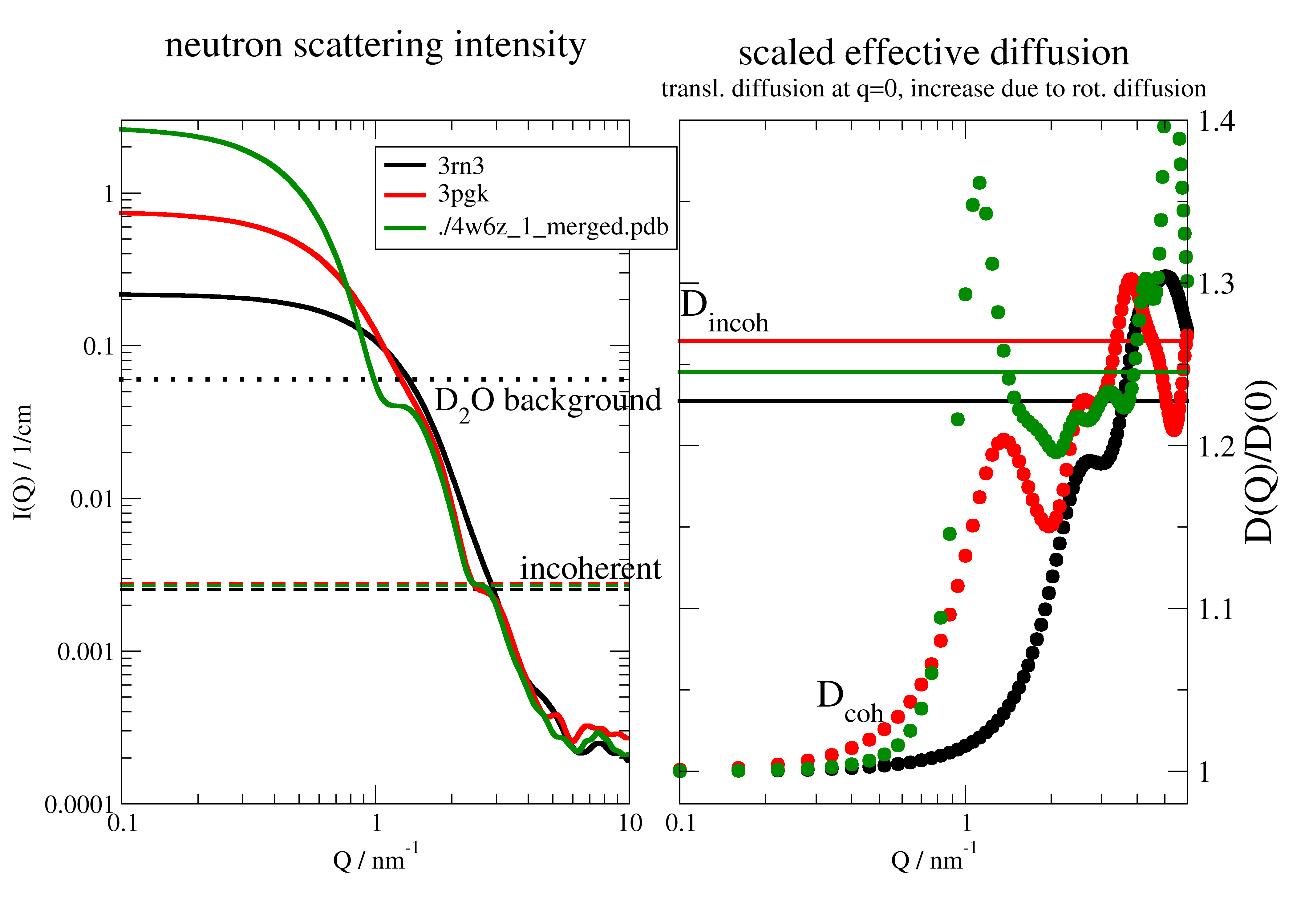
p[0].title('neutron scattering intensity')
p[1].title('scaled effective diffusion')
p[1].subtitle('transl. diffusion at q=0, increase due to rot. diffusion')
p[1].text(r'D\sincoh', x=0.1, y=1.28, charsize=1.5)
p[1].text(r'D\scoh', x=0.3, y=1.04, charsize=1.5)
p[0].text('incoherent', x=3.7, y=0.003, charsize=1.3)
p[0].text(r'D\s2\NO background', x=1.7, y=0.038, charsize=1.3)
# p.save('bio_protein_formfactor+Diffusion.png')
The coherent scattering reflects the shape of the protein at low Q (SANS region) while for \(Q>3 nm^{-1}\) the internal structure is visible (typical backscattering or TOF instruments). For \(Q>>3 nm^{-1}\) the coherent contribution levels between 10-20% of the incoherent scattering for all proteins. The incoherent is slightly dependent on protein amino acid composition but the coherent/incoherent ratio is independent on concentration. The relative D2O background depends on protein concentration.
Above \(Q>>10 nm^{-1}\) the usage of Babinets principle may be questionable and a different calculation method is needed.
\(D_{coh}/D_0\) reflects the shape and size of the protein like the I(Q) does. The incoherent diffusion equals the coherent at larger Q and \(D_{inc}/D_0\) depends slightly on shape. Dependent on the used instrument coherent and incoherent diffusion have to be mixed according to the coherent and incoherent contributions to I(Q). E.g for NSE there is a Q where coherent and incoherent (adds negative) compensate and no signal remains. Often for incoherent measurements only incoherent is taken into account.
Normal mode relaxation as seen by NSE measuring the intermediate scattering function
Alcohol dehydrogenase (yeast) example for normal mode analysis in time domain (NSE)
See Direct Observation of Correlated Interdomain Motion in Alcohol Dehydrogenase for corresponding measurements that show the dynamics.
- In this example we consecutively
Examine the protein
Create normal modes
Calc effective diffusion
Calc the dynamic mode formfactor from normal modes
Show how the intermediate scattering function (ISF) looks with diffusion and internal normal mode relaxation
Finally, we build from this a model that can be used for fitting including H(Q)/S(Q) correction.
# create universe with protein inside that adds hydrogen
# - load PDB structure
# - repair structure e.g. missing atoms
# - add hydrogen using pdb2pqr, saving this to 3cln_h.pdb
# - adds scattering amplitudes, volume determination
%matplotlib
import jscatter as js
import numpy as np
adh = js.bio.fetch_pdb('4w6z.pdb1')
# the 2 dimers in are in model 1 and 2 and need to be merged into one.
adhmerged = js.bio.mergePDBModel(adh)
u = js.bio.scatteringUniverse(adhmerged)
u.atoms.deuteration = 0
protein = u.select_atoms("protein")
S0 = js.bio.nscatIntUniv(protein, cubesize=0.5, getVolume='once')
# ## Calc effective diffusion with trans/rot contributions
# - determine $D_{trans}$ and $D_{rot}$ using HULLRAD
# - calc Deff
D_hr = js.bio.hullRad(u)
Dt = D_hr['Dt'] * 1e2 # conversion to nm²/ps
Dr = D_hr['Dr'] * 1e-12 # conversion to 1/ps
u.qlist = np.r_[0.01, 0.1:3:0.2]
Deff = js.bio.diffusionTRUnivTensor(u.residues, DTT=Dt, DRR=Dr, cubesize=0.5)
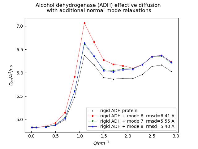
p=js.mplot()
p.Plot(Deff.X, Deff.Y*1e5, li=1, le='rigid ADH protein')
p.Xaxis(label='$Q / nm^{-1}$')
p.Yaxis(label='$D_{eff} /A^2/ns$')
# ## Create normal modes based on residues
nm = js.bio.vibNM(protein.residues,k_b=418)
# ### Normal mode relaxation in small displacement approximation
Ph678 = js.dL()
for NN in [6,7,8]:
Ph = js.bio.intScatFuncPMode(nm, NN, output=0, qlist=Deff.X)
Ph678.append(Ph)
# ## effective diffusion Deff in initial slope (compare to cumulant fit)
a=100.
rate = 1/30000 # 1/ps
for Ph in Ph678:
d = Deff.interp(Ph.X) + rate * a**2 * Ph._Pn / (Ph._Fq+a**2*Ph._Pn) / Ph.X**2
p.Plot(Ph.X,1e5*d ,li='', le=f'rigid ADH + mode {Ph.modeNumber} rmsd={Ph.kTrmsd*a:.2f} A')
p.Title('Alcohol dehydrogenase (ADH) effective diffusion \nwith additional normal mode relaxations')
p.Legend(x=1.5,y=5.5)
# p.savefig(js.examples.imagepath+'/ADHNM_Deff.jpg', dpi=100)
# Assume a common relaxation on top of diffusion
# that we add to Deff
u.qlist = np.r_[0.2:2:0.2] # [1/nm]
u.tlist = np.r_[1, 10:1e5:50] # [ps]
Iqt = js.bio.intScatFuncYlm(u.residues,Dtrans=Dt,Drot=Dr,cubesize=1,getVolume='once')
# ### dynamic mode formfactor P() and relaxation in small displacement approximation with amplitude A(Q)
sumP = Ph678.Y.array.sum(axis=0)
def Aq(a):
# NM mode formfactor amplitude sum
aq = a**2*sumP / (Ph678[0]._Fq + a**2*sumP)
return js.dA(np.c_[Ph678[0].X, aq].T)
p2=js.mplot()
p2.Yaxis(min=0.01, max=1, label='I(Q,t)/I(Q,0)')
p2.Xaxis(min=0, max=100000, label='t / ps')
Iqt2 = Iqt.copy()
l=1/10000 # 1/ps
Aqa = Aq(a)
for i, qt in enumerate(Iqt2):
diff = qt.Y *(1-Aqa.interp(qt.q))
qt.Y = qt.Y *((1-Aqa.interp(qt.q)) + Aqa.interp(qt.q)*np.exp(-l*qt.X))
p2.Plot(qt.X, qt.Y * 0.8**i,sy=0,li=[3,2,i+1],le=f'{qt.q:.1f}')
p2.Plot(qt.X, diff* 0.8**i,sy=0,li=[1,2,i+1])
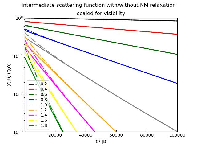
p2.Yaxis(min=0.001,max=1,label='I(Q,t)/I(Q,0)',scale='log')
p2.Xaxis(min=0.1,max=100000,label='t / ps')
p2.Title('Intermediate scattering function with/without NM relaxation')
p2.Subtitle('scaled for visibility')
p2.Legend()
# p2.savefig(js.examples.imagepath+'/ADHNM_Iqt.jpg', dpi=100)
if 0 :
# look at A(Q)
p1=js.mplot()
Aqa = Aq(a)
p1.Plot(Aqa, sy=0, li=1)
p1.Yaxis(min=0, max=0.8)
The ISF shows in the initial slope the combined Deff and relaxes for longer times > 30ns to the rigid protein Deff.
How strong the change is depends on the mode amplitudes and the relaxation times of the modes.
For the model we use the ISF of multiple modes (see intScatFuncPMode())
and the Rayleigh expansion for diffusing rigid proteins/particles (intScatFuncYlm()) :
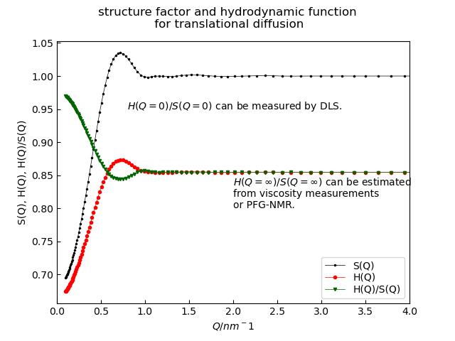
Translational and rotational diffusion are corrected for direct interparticle interactions described by the structure factor \(S(Q)\) and hydrodynamic interactions within the hydrodynamic function \(H(Q)\) as \(D_t(Q) = D_{t,0} H(Q)/S(Q)\) and \(D_r = D_{r.0}H_r\).
The intermediate scattering function \(F(Q)\) assuming dynamic decoupling with translational/rotational and domain motions is
trans/rot diffusion contribution
\[F_{t,r}(Q,t) = e^{-D_{t}Q^2t}\sum_l S_l(Q)e^{-l(l+1)D_{r}t}\]normal mode contributions
\[\begin{split}F_a(Q,t) &= \frac{F(Q) + \sum_{\alpha} e^{-\lambda_{\alpha} t} P_{\alpha}(Q)}{[F(Q) + \\ \sum_{\alpha} P_{\alpha}(Q)]} &= (1-A(Q)) + A(Q) e^{-\lambda t}\end{split}\]with with common relaxation rate \(\lambda\) and \(A(Q) = \frac{\sum_{\alpha} P_{\alpha}(Q)}{[F(Q) + \sum_{\alpha} P_{\alpha}(Q)]}\)
We can also use the Ornstein-Uhlenbeck like relaxation
intScatFuncOU()for \(F_a(Q,t)\) that allows description within internal friction in the protein. The above description corresponds to a small displacement approximation of the Ornstein-Uhlenbeck process.
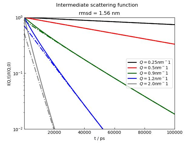
Finally NSE data can be read including Q values like IN15 or JNSE. Typically we measure 10-15 different Q values between \(0.025-0.2 nm^{-1}\). The read dataList should contain for each dataArray an attribute q with the scattering vector. For demonstration we just use simulated data here
# A fit model to fit Iqt from NSE measurements
# Include H(Q) and S(Q)
# and repeat what we need from part 1

%matplotlib
import jscatter as js
import numpy as np

# create universe
adh = js.bio.fetch_pdb('4w6z.pdb1')
adhmerged = js.bio.mergePDBModel(adh)
u = js.bio.scatteringUniverse(adhmerged)
u.setSolvent('1d2o1')
u.qlist = js.loglist(0.1, 5, 100)
u.atoms.deuteration = 0
protein = u.select_atoms('protein')
S0 = js.bio.nscatIntUniv(protein, cubesize=0.5, getVolume='once')


# structure factor Sq and hydrodynamic function Hq
# This should be determined from SAXS/SANS measurements at same concentration like NSE
# and maybe fit including concentration dependence
mol = 0.0003
R=4
def Sqbeta(q, R, molarity):
    # this function should be used for structure factor fitting of experimental data
    # as it contains the shape correction from Kotlarchyk and S.-H. Chen, J. Chem. Phys. 79, 2461 (1983)
    # structure factor without correction
    Sq = js.sf.PercusYevick(q=q, R=R, molarity=molarity)  # about 50mg/ml protein like experimental data
    # factor beta from formfactor calculation
    beta = S0.interp(q, col='beta')
    # correct Sq for beta
    Sq.Y = 1 + beta * (Sq.Y-1)
    return Sq

# Hq can be determined by fitting Rh or be determined by other measurements
# We assume here larger hydrodynamic interaction
# The Kotlarchyk correction from above is included by using Sqbeta
Hq = js.sf.hydrodynamicFunct(S0.X, Rh=R*1.1, molarity=mol,
                             structureFactor=Sqbeta,
                             structureFactorArgs={'R': R}, )


# look at the  D_t = D_0 H(Q)/S(Q) correction for translational diffusion
p3 = js.mplot()
p3.plot(Hq.X,Hq._sf,le='S(Q)')
p3.plot(Hq,le='H(Q)')
p3.plot(Hq.X, Hq.Y/Hq._sf,le='H(Q)/S(Q)')
p3.Yaxis(label='S(Q), H(Q), H(Q)/S(Q)')
p3.Xaxis(min=0.,max=4,label='$Q / nm^-1$')
p3.Title('structure factor and hydrodynamic function\n for translational diffusion')
p3.Text('$H(Q=\infty)/S(Q=\infty)$ can be estimated \nfrom viscosity measurements \nor PFG-NMR.',x=2,y=0.8)
p3.Text('$H(Q=0)/S(Q=0)$ can be measured by DLS.',x=0.8,y=0.95)
p3.Legend()
# p3.savefig(js.examples.imagepath+'/ADHNM_SqHq.jpg', dpi=100)

D_hr = js.bio.hullRad(u)
Dt = D_hr['Dt'] * 1e2  # conversion to nm²/ps
Dr = D_hr['Dr'] * 1e-12  # conversion to 1/ps
# u.qlist = np.r_[0.01, 0.1:3:0.2]
Deff = js.bio.diffusionTRUnivTensor(u.residues, DTT=Dt, DRR=Dr, cubesize=0.5)

# make normal modes and calc A(Q)
ca = u.residues
nm = js.bio.vibNM(ca)
Ph678 = js.dL()
for NN in [6,7,8]:
   Ph = js.bio.intScatFuncPMode(nm, NN, output=0, qlist=Deff.X)
   Ph678.append(Ph)
sumP = Ph678.Y.array.sum(axis=0)


def Aq(a):
    aq = a**2*sumP / (Ph678[0]._Fq + a**2*sumP)
    A = js.dA(np.c_[Ph678[0].X, aq].T)
    A.rmsdNM = a * Ph678.kTrmsdNM.array.sum()
    return A

# this is the model for a fit
def transRotModes(t, q, Dt, Dr, Rhf=1, R=4, a=1000, l=10, mol=0.0003):
    # trans rot diffusion including H(Q)/S(Q)
    # default values for R, mol are determined from preparation or experiments

    Sq = Sqbeta(q=q, R=R, molarity=mol)
    # assume a factor between the interaction radius R and hydrodynamic radius Rh
    Hq = js.sf.hydrodynamicFunct(q, Rh=R*Rhf, molarity=mol, structureFactor=Sqbeta,
                                structureFactorArgs={'R': R}, )

    Dth = Dt * Hq.interp(q) / Sq.interp(q)
    # assume Hr =1-(1-DsoverD0)/3 for rotational diffusion
    Drh = Dr*(1-(1-Hq.DsoverD0)/3)
    Iqt = js.bio.intScatFuncYlm(u.residues, qlist=np.r_[q],tlist=t, Dtrans=Dth, Drot=Drh, cubesize=1)[0]

    # add Pmode relaxation
    Aqa = Aq(a)
    diff = Iqt.Y *(1-Aqa.interp(q))
    Iqt.Y = Iqt.Y *((1-Aqa.interp(q)) + Aqa.interp(q)*np.exp(-1/(l*1000)*Iqt.X))
    Iqt2 = Iqt.addColumn(1,diff)

    # for later reference in lastfit save parameters
    Iqt2.Dt = Dt
    Iqt2.Dr = Dr
    Iqt2.H0= Hq.DsoverD0
    Iqt2.R = R
    Iqt2.Rh = R * Rhf
    Iqt2.rmsdNM = Aqa.rmsdNM

    return Iqt2

# simulate data
tlist = np.r_[1, 10:1e5:50]
sim = js.dL()
for q in np.r_[0.25,0.5,0.9,1.2,2]:
    sim.append(transRotModes(t=tlist, q=q, Dt=Dt, Dr=Dr,a=100,l=10))

p4=js.mplot()
for c, si in enumerate(sim,1):
    p4.plot(si,sy=0,li=[1,2,c],le=f'$Q={si.q} nm^{-1}$')
    p4.plot(si.X,si[2], sy=0, li=[3,2,c ])
p4.Yaxis(min=0.01,max=1,label='I(Q,t)/I(Q,0)',scale='log')
p4.Xaxis(min=0.1,max=100000,label='t / ps')
p4.Title('Intermediate scattering function')
p4.Subtitle(f'rmsd = {si.rmsdNM:.2f} nm')
p4.Legend()
# p4.savefig(js.examples.imagepath+'/ADHNM_IQTsim.jpg', dpi=100)

if 0:
    # A fit to exp. NSE data might be done like this (using sim as measured data)
    # fixpar are determined from other experiments (e.g. Dt0 extrapolating DLS to zero conc.)
    # or Dr0 from calculation from structure (using HULLRAD or HYDROPRO), mol from sample preparation
    Dt0 = 4.83e-05   #  nm²/ps
    Dr0 = 1.64e-06  #  1/ps
    sim.fit(model=transRotModes,
                freepar={'Rhf':1, 'a':100, 'l':10},
                fixpar={'Dt':Dt0, 'Dr':Dr0,'R':4, 'mol':0.0003 },
                mapNames={'t':'X'})
Load trajectory from MD simulation
A scatteringUniverse with a complete trajectory from MD simulation is created. The PSF needs atomic types to be guessed from names to identify atoms in the used format. You may need to install MDAnalysisTests to get the files.( python -m pip install MDAnalysisTests)
It might be necessary to transform the box that the protein is not crossing boundaries of the universe box.
from MDAnalysisTests.datafiles import PSF, DCD
import jscatter as js
import numpy as np
import MDAnalysis as mda
from MDAnalysis.topology.guessers import guess_types
upsf1 = js.bio.scatteringUniverse(PSF, DCD, assignTypes={'from_names':1})
upsf1.view(frames="all")
upsf1.setSolvent('1d2o1')
upsf1.qlist = js.loglist(0.1, 5, 100)
Sqtraj = js.dL()
# select protein and not the solvent if this is present
protein = upsf1.select_atoms('protein')
if 0:
# only if needed to avoid crossing boundaries
# add a transform that puts the protein into the center of the box and wrap the solvent into the new box
# for details see MDAnalysis Trajectory transformations
protein = upsf1.select_atoms('protein')
not_protein = upsf1.select_atoms('not protein')
transforms = [trans.unwrap(protein),
trans.center_in_box(protein, wrap=True),
trans.wrap(not_protein, compound='fragments')]
# now loop over trajectory
for ts in upsf1.trajectory[2::13]:
Sq = js.bio.nscatIntUniv(protein)
Sq.time = upsf1.trajectory.time
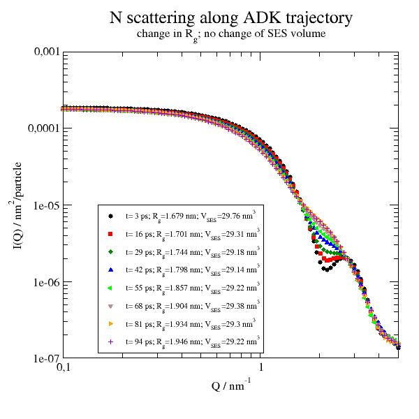
print(Sq.RgInt)
Sqtraj.append(Sq)
# show
p = js.grace()
p.title('N scattering along ADK trajectory')
p.subtitle(r'change in R\sg\N; no change of SES volume')
p.yaxis(scale='l',label=r'I(Q) / nm\S2\N/particle')
p.xaxis(scale='l',label='Q / nm\S-1')
p.plot(Sqtraj,le=r't= $time ps; R\sg\N=$RgInt nm; V\sSES\N=$SESVolume nm\S3')
p.legend(x=0.15,y=1e-5,charsize=0.7)
# p.save(js.examples.imagepath+'/uniformfactorstraj.jpg', size=(2, 2))
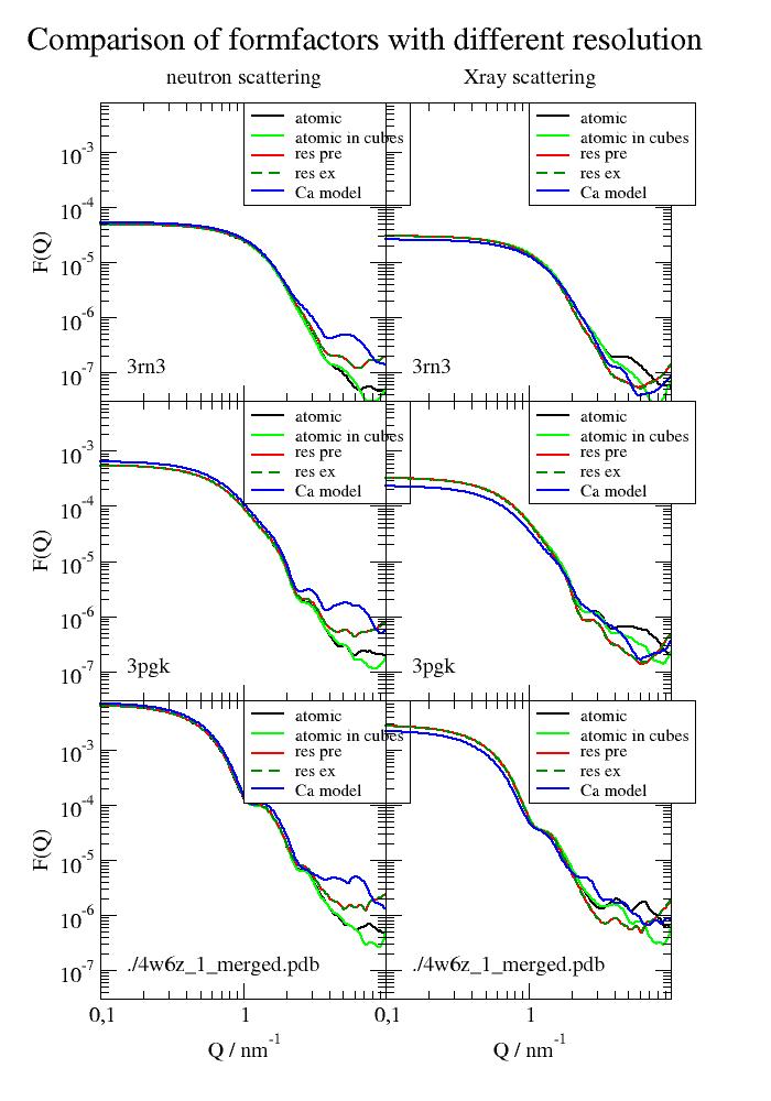
Compare different resolution options for coarse graining
PDB structures without explicit solvent for small angle scattering.
The example shows the validity of residue coarse graining up to around 3/nm. With coarse graining in cubes (cubesize) the approximation seems best. This might be useful to speed up computations that take long (e.g. ISF at low Q)
There is basically no difference between precalculated and averaged residue formfactors and explicit calculated residue formfactors for each residue (uni.explicitResidueFormFactorAmpl = True) The explicit ones include better deuteration of specific atoms.
Cα models loose some precision in volume respectively in forward scattering. C-alpha models need a .calphaCoarseGrainRadius = 0.342 nm because of the missing atoms. In addition, the mean residue position is not the C-alpha position. We use 0.342 nm as a good average to get same forward scattering over a bunch of proteins (see example_bio_proteinCoarseGrainRadius.py).
import jscatter as js

# first get and create the biological unit ('.pdb1') of alcohol dehydrogenase (tetramer, 144 kDa)
adh = js.bio.fetch_pdb('4w6z.pdb1')
# the 2 dimers in are in model 1 and 2 and need to be merged into one.
adhmerged = js.bio.mergePDBModel(adh)

# Ribonuclease A and Phosphoglycerate kinase are monomers and can be used without modifications.
# 3pgk has a Mg atom that is misinterpreted (as M), to use it we add this
vdwradii = {'M': js.data.vdwradii['Mg'] * 10}  # in A

p = js.grace(1, 1.4)
p.multi(3, 2, vgap=0, hgap=0)
for c, pdbid in enumerate(['3rn3', '3pgk', adhmerged]):
    # load from pdb id, scatteringUniverse adds hydrogens automatically
    uni = js.bio.scatteringUniverse(pdbid, vdwradii=vdwradii)
    uni.setSolvent('1d2o1')
    uni.qlist = js.loglist(0.1, 9.9, 200)
    u = uni.select_atoms("protein")
    ur = u.residues

    S = js.bio.nscatIntUniv(u)
    Sx = js.bio.xscatIntUniv(u)

    # use an averaging in cubes filled with the atoms, cubesize approximates residue size
    Scu = js.bio.nscatIntUniv(u, cubesize=0.6)
    Sxcu = js.bio.xscatIntUniv(u, cubesize=0.6)

    # use now the precalculated formfactors on residue level coarse graining
    uni.explicitResidueFormFactorAmpl = False  # default
    Sr = js.bio.nscatIntUniv(ur)
    Sxr = js.bio.xscatIntUniv(ur)

    # calc residue formfactors explicit (not precalculated)
    # useful for changes of residue deuteration or backbone N-H exchange of IDP
    uni.explicitResidueFormFactorAmpl = True
    Ser = js.bio.nscatIntUniv(ur)
    Sxer = js.bio.xscatIntUniv(ur)

    # create a C-alpha pdb file and then the Ca-only universe for calculation
    ca = uni.select_atoms('name CA')
    ca.write('pdb_ca.pdb')
    # addHydrogen=False prevents addition of 4H per C atom
    unica = js.bio.scatteringUniverse('pdb_ca.pdb', addHydrogen=False)
    # To use precalculated residue formfactors explicit... should be False
    unica.explicitResidueFormFactorAmpl = False
    unica.setSolvent('1d2o1')
    unica.qlist = js.loglist(0.1, 10, 200)
    uca = unica.residues
    Sca = js.bio.nscatIntUniv(uca, getVolume='now')
    Sxca = js.bio.xscatIntUniv(uca)

    p[2 * c].plot(S, li=[1, 2, 1], sy=0, le='atomic')
    p[2 * c].plot(Scu, li=[1, 2, 5], sy=0, le='atomic in cubes')
    p[2 * c].plot(Sr, li=[1, 2, 2], sy=0, le='res pre')
    p[2 * c].plot(Ser, li=[3, 2, 3], sy=0, le='res ex')
    p[2 * c].plot(Sca, li=[1, 2, 4], sy=0, le='Ca model')
    p[2 * c].legend(x=1, y=8e-3, charsize=0.8)
    p[2 * c].text(x=0.15, y=1e-7, charsize=1, string=pdbid)

    p[2 * c + 1].plot(Sx, li=[1, 2, 1], sy=0, le='atomic')
    p[2 * c + 1].plot(Sxcu, li=[1, 2, 5], sy=0, le='atomic in cubes')
    p[2 * c + 1].plot(Sxr, li=[1, 2, 2], sy=0, le='res pre')
    p[2 * c + 1].plot(Sxer, li=[3, 2, 3], sy=0, le='res ex')
    p[2 * c + 1].plot(Sxca, li=[1, 2, 4], sy=0, le='Ca model')
    p[2 * c + 1].legend(x=1, y=8e-3, charsize=0.8)
    p[2 * c + 1].text(x=0.15, y=1e-7, charsize=1, string=pdbid)

    p[2 * c].xaxis(label='', ticklabel=False, scale='log', min=1e-1, max=9.9)
    p[2 * c + 1].xaxis(label='', ticklabel=False, scale='log', min=1e-1, max=9.9)
    p[2 * c].yaxis(label='F(Q)', ticklabel='power', scale='log', min=3e-8, max=8e-3)
    p[2 * c + 1].yaxis(ticklabel=False, scale='log', min=3e-8, max=8e-3)

p[2 * c].xaxis(label=r'Q / nm\S-1', ticklabel=True, scale='log', min=1e-1, max=9.9)
p[2 * c + 1].xaxis(label=r'Q / nm\S-1', ticklabel=True, scale='log', min=1e-1, max=9.9)
p[0].subtitle('neutron scattering')
p[1].subtitle('Xray scattering')
p[0].title(' ' * 30 + 'Comparison of formfactors with different resolution')
# p.save(js.examples.imagepath+r'/uniformfactors.jpg', size=(700/300, 1000/300))
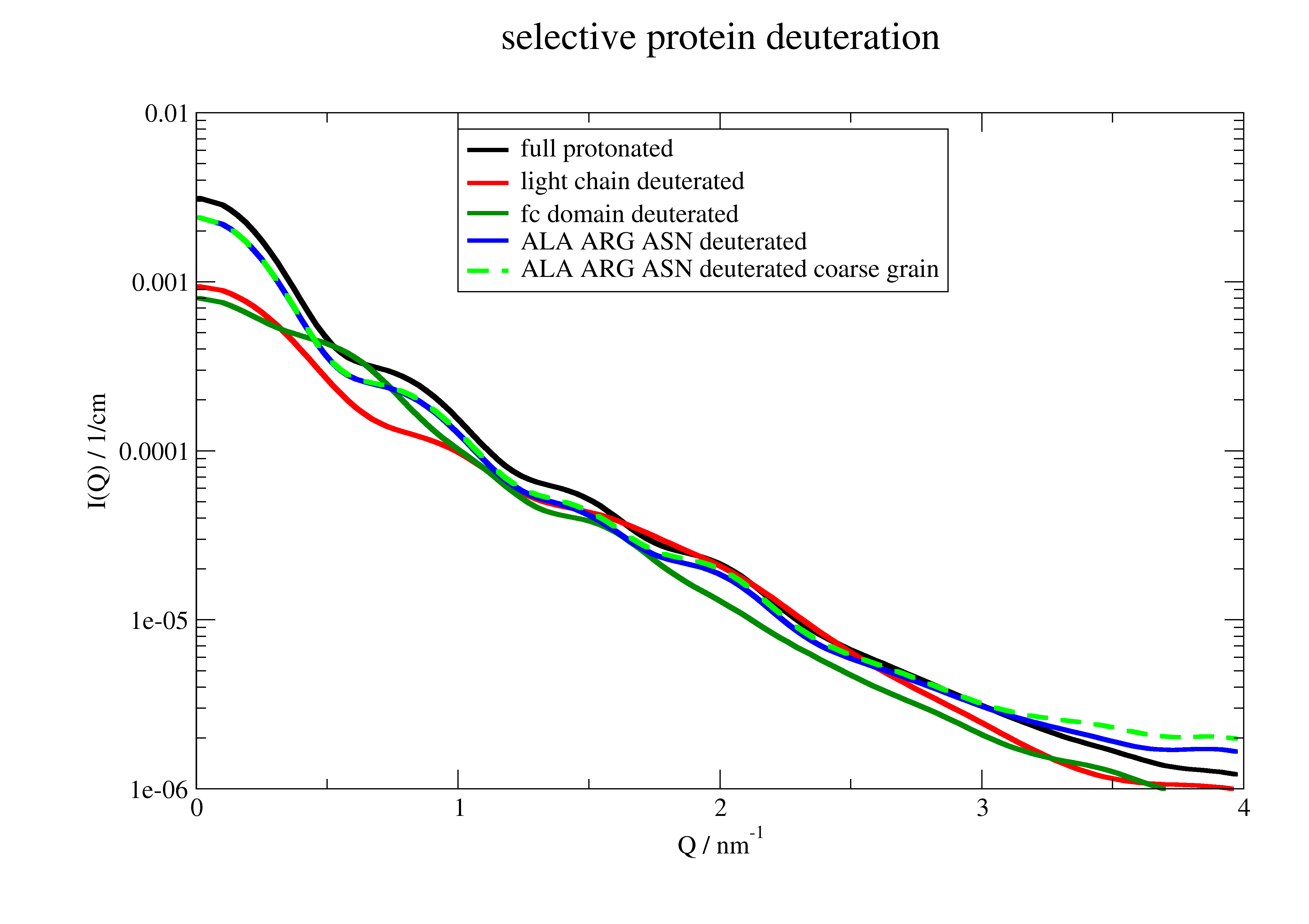
Selective partial deuteration
Partial deuteration of protein complexes is a promising tool for examination of protein structure function relationship. E.g. see an interesting example about the complex in the cyanobacterial circadian clock system Sugiyama et al, Nature Communications Biology (2022). https://doi.org/10.1038/s42003-022-03143-z
Here we see how to selectively deuterate domains or specific aminoacids and how scattering is influenced. The deuteration is considered in all bio methods.
import jscatter as js
import numpy as np
import scipy.constants as constants

# create universe
mab = js.bio.scatteringUniverse('1igt')
mab.setSolvent('1d2o1')

mab.qlist = np.r_[0.01, 0.1:4:0.03]
# use explicit residue formfactors for EACH residue
mab.explicitResidueFormFactorAmpl = True

# use a atom selection
lightchains = mab.select_atoms('segid A C')  # light chains

mab.atoms.deuteration = 0  # default protonated
I_protonated = js.bio.nscatIntUniv(mab.atoms)

lightchains.atoms.deuteration = 1
I_lightdeuterated = js.bio.nscatIntUniv(mab.atoms)

mab.atoms.deuteration = 0
# select fc domain
mab.select_atoms('segid B D and resid 240-700').deuteration = 1
I_fcdeuterated = js.bio.nscatIntUniv(mab.atoms)

mab.atoms.deuteration = 0
# select 3 residue
mab.select_atoms('resname ALA ARG ASN ').deuteration = 1
I_someAA = js.bio.nscatIntUniv(mab.atoms)
#

I_someresidue = js.bio.nscatIntUniv(mab.residues)

p = js.grace()
p[0].plot(I_protonated, sy=0, li=[1, 3, 1], le='full protonated')
p[0].plot(I_lightdeuterated, sy=0, li=[1, 3, 2], le='light chain deuterated')
p[0].plot(I_fcdeuterated, sy=0, li=[1, 3, 3], le='fc domain deuterated')
p[0].plot(I_someAA, sy=0, li=[1, 3, 4], le='ALA ARG ASN deuterated')
p[0].plot(I_someresidue, sy=0, li=[3, 3, 5], le='ALA ARG ASN deuterated coarse grain')


p.xaxis(label=r'Q / nm\S-1', min=0, max=4)
p.yaxis(label=r'I(Q) / 1/cm', scale='log', min=1e-6, max=0.01)
p.legend(x=1, y=0.008)
p.title('selective protein deuteration')

# p.save('bio_protein_partialmatching.png')
A protein normal mode animation
Creating a trajectory from normal modes and show I(Q) together with the configuration.
The calculation can also be done along a MD simulation in .trajectory .
MDAnalysis allows a bunch of trajectory manipulations like center of mass removal or rotations.
import jscatter as js
import numpy as np
import tempfile
import os
import pymol2
import matplotlib.image as mpimg


def savepng(u, fname):
    """Save png image from pymol"""
    p1 = pymol2.PyMOL()
    p1.start()
    with tempfile.TemporaryDirectory() as tdir:
        name = os.path.splitext(u.filename)[0] + '.pdb'
        tfile = os.path.join(tdir, name)
        u.atoms.write(tfile)
        p1.cmd.load(tfile)
        p1.cmd.rotate('x', 90, 'all')
        p1.cmd.color('red', 'ss h')
        p1.cmd.color('yellow', 'ss s')
        p1.cmd.color('blue', 'ss l+')
        p1.cmd.set('cartoon_discrete_colors',1)
        p1.cmd.png(fname, width=600, height=600, dpi=-1, ray=1)
    p1.stop()


uni=js.bio.scatteringUniverse(js.examples.datapath+'/arg61.pdb', addHydrogen=False)

uni=js.bio.scatteringUniverse('3pgk')
uni.setSolvent('1d2o1')
u = uni.select_atoms("protein and name CA")
# create normal modes
nm = js.bio.vibNM(u)
# make a trajectory similar to a MD simulation
moving = nm.animate([6,7,8,9], scale=120)
moving.qlist = js.loglist(0.1, 5, 100)

p = js.mplot(16, 8)
# loop over trajectory timesteps
for i, ts in enumerate(moving.trajectory):
    # calc th scattering and plot it
    Sq = js.bio.xscatIntUniv(moving.atoms, refreshVolume=False)
    p.Multi(1, 2)
    p[1].axis('off')
    p[0].Plot(Sq, li=[1,2,1], sy=0)
    p[0].Yaxis(label='F(Q) / nm²', scale='log', min=3e-7, max=6e-4)
    p[0].Xaxis(label=r'$Q / nm^{-1}$')
    name = f'test_{i:.0f}.png'
    savepng(moving, name)
    img = mpimg.imread(name)
    p[1].imshow(img)
    # p.savefig(name, transparent=True, dpi=100)
    p.clear()

p.Close()

# In Ipython use ImageMagic to generate animated gif
# %system convert -delay 10 -loop 0  -dispose Background test*.png mode_animation.gif
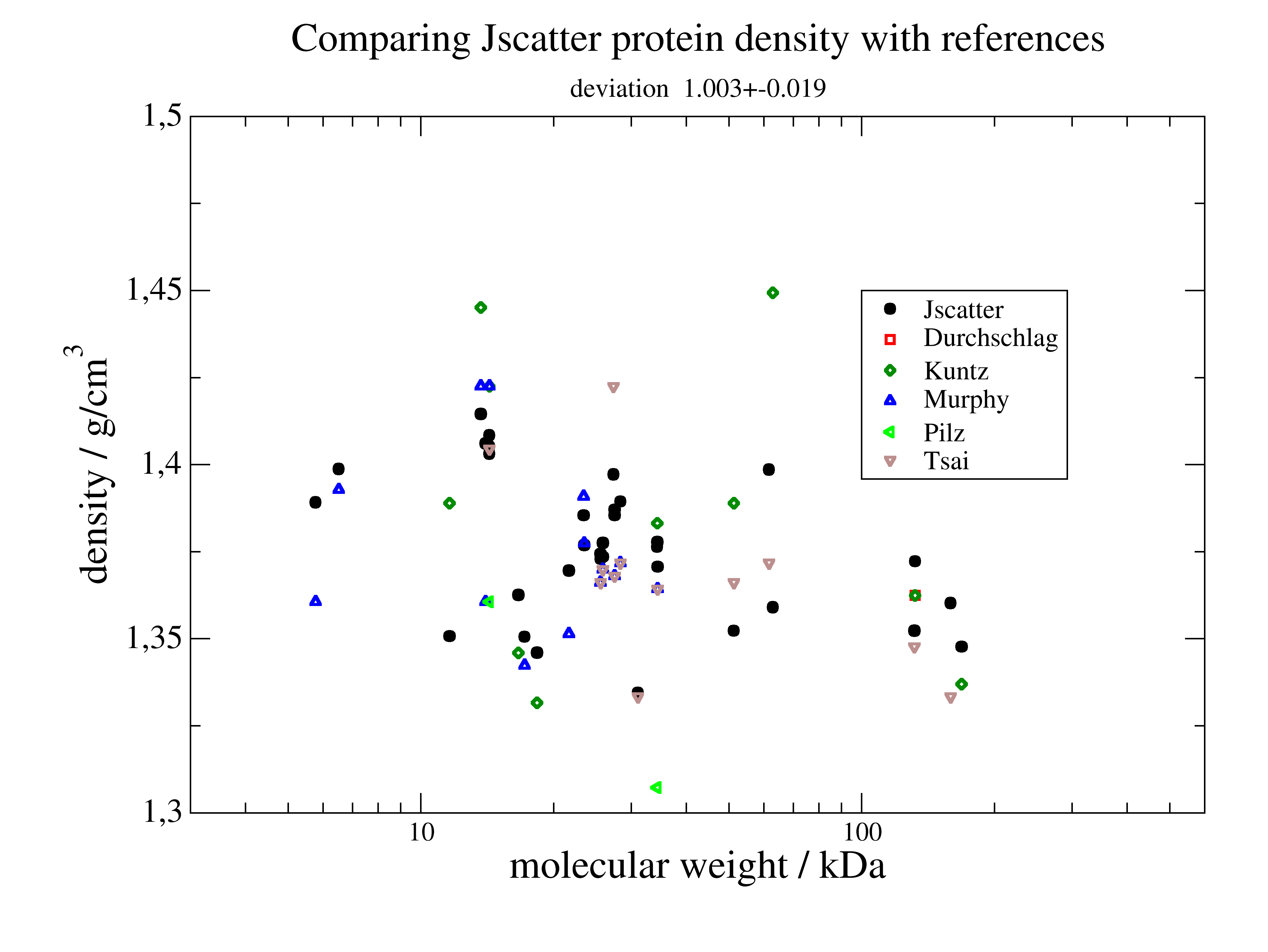
Protein density determination
We compare measured protein density data with the density calculated by Jscatter
to check the SESVolume accuracy in the module jscatter.bio .
Respective references are given in js.examples.datapath+'/proteinSpecificVolumes.txt'
import os.path
import jscatter as js
import numpy as np

# Comparison of the calculated protein density with several references

# read partial specific volumes
with open(js.examples.datapath+'/proteinSpecificVolumes.txt') as f:
    lines = f.readlines()

universes = []
for line in lines:
    words = line.split()
    if len(words)==0 or words[0].startswith('#'):
        continue
    print(words)
    author = words[3]
    if os.path.exists(words[1]+'_h.pdb'):
        uni = js.bio.scatteringUniverse(words[1]+'_h.pdb', addHydrogen=False)
    else:
        uni = js.bio.scatteringUniverse(words[1])
    uni.densityPaper= 1/float(words[2])
    uni.qlist = js.loglist(0.1, 4, 40)
    uni.solvent = ['0D2O1', '1H2O1']
    uni.pdb = words[1]
    uni.author = author
    universes.append(uni)

Slist = js.dL()
for uni in universes:
    uni.probe_radius = 0.13
    u = uni.select_atoms("protein")
    S = js.bio.scatIntUniv(u, mode='xray')
    S.densityPaper = uni.densityPaper
    S.author = uni.author
    Slist.append(S)

p=js.grace()
p.plot(Slist.mass.array/1000., Slist.massdensity, sy=[1, 0.5, 1, 1], le='Jscatter')
for c, author in enumerate(Slist.author.unique, 2):
    Sl = Slist.filter(author=author)
    p.plot(Sl.mass.array/1000., Sl.densityPaper.array, sy=[c, 0.5, c], le=author)
dev = Slist.massdensity/Slist.densityPaper.array
p.xaxis(min=3, max=600, label=r'molecular weight / kDa', charsize=1.5, scale='log')
p.yaxis(label=r'density / g/cm\S3\N', charsize=1.5)
st = fr'Mean density {Slist.densityPaper.mean:.2f}+-{Slist.densityPaper.std:.2f} g/cm\S3\N;' \
      +fr' Jscatter deviation  {dev.mean():.3f}+-{dev.std():.3f}'
p.subtitle(st)
p.title(r'Comparing Jscatter protein density with references ')
p.legend(x=100, y=1.45)
# p.save('proteinDensityTest.png')
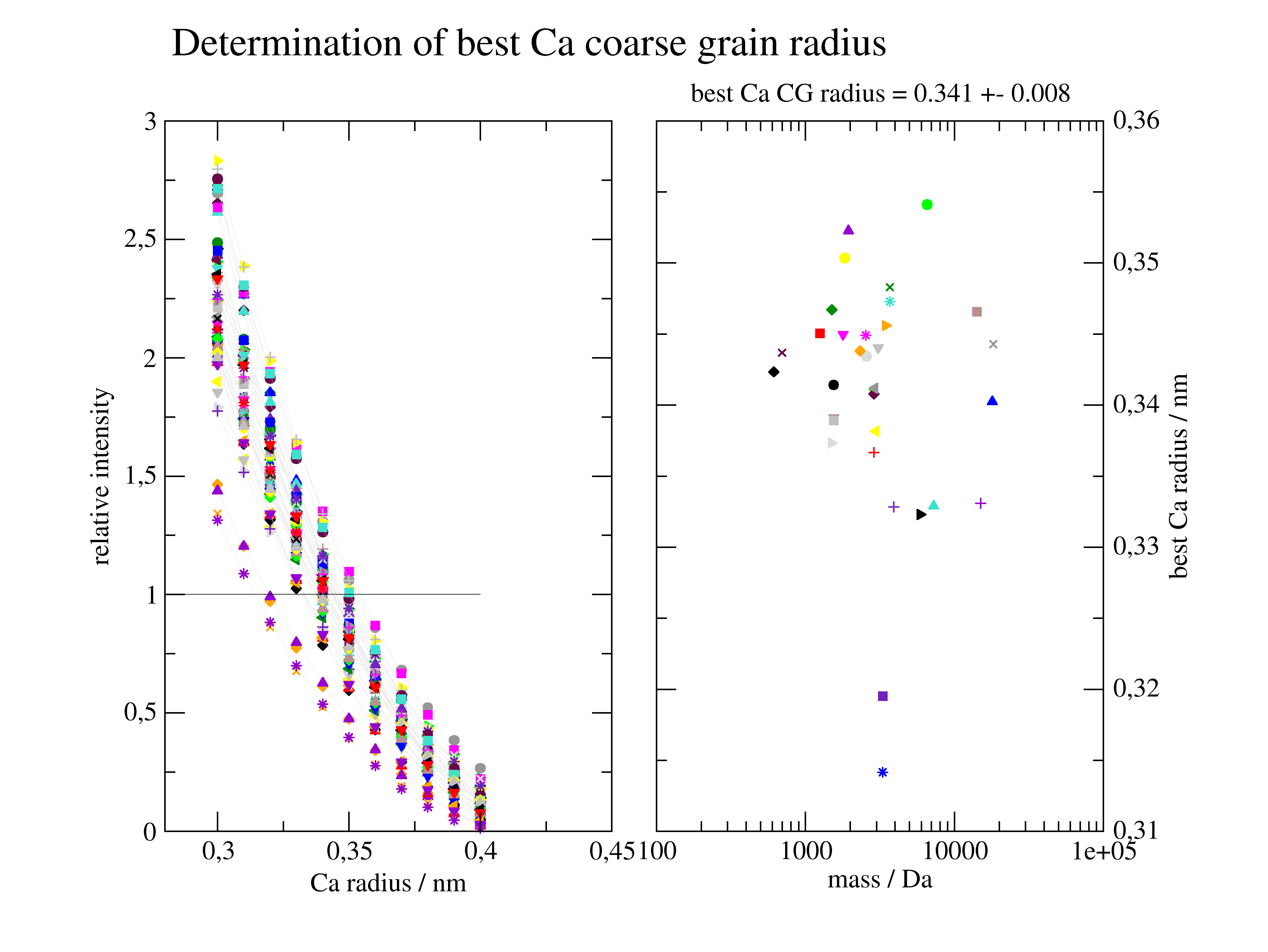
Cα coarse grain radius
We calculate an appropriate Size of residues dummy atoms for Cα atom models to get a reasonable protein scattering intensity.
"""
This test determines the best calphaCoarseGrainRadius to result in
best approximated forward scattering I0 of the selected proteins.

The best result is for calphaCoarseGrainRadius = 0.362

Dependent on the protein structure slightly different values might be better.
But anyway bead models and Cα models are always a rough approximation.

"""
import jscatter as js
import numpy as np
import os

with open(js.examples.datapath + '/proteinSpecificVolumes.txt') as f:
    lines = f.readlines()

vdw = {'CO': 0.15, 'Z': js.data.vdwradii['Zn'] * 10, 'M': js.data.vdwradii['Mg'] * 10}

Slist = js.dL()
for line in lines:
    words = line.split()
    if len(words)==0 or words[0].startswith('#'):
        continue
    if len(Slist)>0 and words[1] in Slist.proteinID:
        continue
    if os.path.exists(words[1]+'_h.pdb'):
        uni = js.bio.scatteringUniverse(words[1]+'_h.pdb', addHydrogen=False)
    else:
        uni = js.bio.scatteringUniverse(words[1])
    u = uni.select_atoms("protein")
    S = js.bio.xscatIntUniv(u)
    ca = uni.select_atoms('name CA')
    ca.write('uniCA.pdb')
    unica = js.bio.scatteringUniverse('uniCA.pdb', addHydrogen=False)
    uca = unica.residues
    pr = np.r_[0.3:0.4:0.01]
    for r in pr:
        print(words[1], r)
        unica.calphaCoarseGrainRadius = r
        Sca = js.bio.xscatIntUniv(uca)
        Sca.relVolume = Sca.SESVolume / S.SESVolume
        Sca.relI0 = Sca.I0 / S.I0
        Sca.atomVolume = S.SESVolume
        Sca.proteinID = words[1]
        Sca.pr = r
        Slist.append(Sca)

p2 = js.grace()
p2.multi(1, 2)
xx = []
for id in Slist.proteinID.unique:
    sl = Slist.filter(proteinID=id)
    rV = js.dA(np.c_[sl.pr, sl.relI0].T)
    rV.fit(lambda x, b, x0: (b * (x - x0) + 1) ** 2, {'b': 11, 'x0': 0.35}, {}, {'x': 'X'})
    p2[0].plot(rV, le=f'{rV.x0:.3f}')
    p2[0].plot(rV.lastfit, li=[1,0.3,11])
    p2[1].plot([sl[0].mass], [rV.x0])
    xx.append(rV.x0)
xx = np.array(xx)
p2[0].plot([0.1, 0.4], [1] * 2, sy=0, li=1)
p2[0].xaxis(label='Ca radius / nm', min=0.28, max=0.45)
p2[0].yaxis(label='relative intensity')
p2[1].xaxis(scale='log', label='mass / Da')
p2[1].yaxis(label=['best Ca radius / nm',1,'opposite'],ticklabel= ['general',2,1,'opposite'])
p2[1].subtitle(f'best Ca CG radius = {np.mean(xx):.3f} +- {np.std(xx):.3f} ')
p2[0].title('                            Determination of best Ca coarse grain radius')
# p2.save('proteinCacoarsegrainRadius.png')

# Conclusion CA model with vdWradius 0.342 is appropriate