3. dataList¶

dataList contain a list of dataArray.

List of dataArrays allowing variable sizes and attributes.
Basic list routines as read/save, appending, selection, filter, sort, prune, interpolate, spline…
Multidimensional least square fit that uses the attributes of the dataArray elements.
Higher dimesions (>1) are in the attributes.
Read/Write in human readable ASCII text of multiple files in one run (gzip possible) or pickle.
A file may contain several datasets and several files can be read.
For programmers: Subclass of list

For Beginners:

Create a dataList and use the methods from this object in point notations.:

data=js.dL('filename.dat').
data.prune(number=100)
data.attr
data.save('newfilename.dat')

The dataList methods should not be used directly from this module.

See dataList for details.

Example:

p=js.grace()
dlist2=js.dL()
x=np.r_[0:10:0.5]
D,A,q=0.45,0.99,1.2
for q in np.r_[0.1:2:0.2]:
   dlist2.append(js.dA(np.vstack([x,np.exp(-q**2*D*x),np.random.rand(len(x))*0.05])) )
   dlist2[-1].q=q
p.clear()
p.plot(dlist2,legend='Q=$q')
p.legend()
dlist2.save('test.dat.gz')

The dataarray module can be run standalone in a new project.

3.1. dataList Class¶

dataList([objekt, block, usecols, ...])

A list of dataArrays with attributes for analysis, fitting and plotting.

dataList creating by dataL=js.dL(‘filename.dat’) or from numpy arrays.
List columns can be accessed as automatic generated attributes like .X,.Y,.eY (see protectedNames). or by indexing as *dataL[:,0] -> .X * for all list elements.
Corresponding column indices are set by setColumnIndex() (default X,Y,eY = 0,1,2).
Multidimensional fitting of 1D,2D,3D (.X,.Z,.W) data including additional attributes. .Y (scalar) are used as function values at coordinates.
Attributes can be set like: dataL.aName= 1.2345 or dataL[2].aName= 1.2345
Individual elements and dataArray methods can be accessed by indexing data[2].bName
Methods are used as dataL.methodname(arguments)

3.2. Attribute Methods¶

`attr`	Returns all attribute names (including commonAttr of elements) of the dataList.
`dlattr`([attr])	Get attribute or list of existing attribute names excluding common attributes from dataArrays.
`commonAttr`	Returns list of attribute names existing in elements.
`dtype`	return dtype of elements
`names`	List of element names.
`whoHasAttributes`	Lists which attribute is found in which element.
`showattr`([maxlength, exclude])	Show data specific attributes for all elements.

3.3. Fit Methods¶

Least square fit and Bayes

`fit`(model[, freepar, fixpar, mapNames, ...])	Least square fit of model that minimizes $\chi^2$ (uses scipy.optimize methods) or Bayesian analysis.
`modelValues`(**kwargs)	Get modelValues allowing simulation with changed parameters.
`estimateError`([method, output])	Estimate error using a refined fit (`method='lm'`) if no error is present.
`refineFit`([method])	Refined fit with starting values from previous fit.
`getBayesSampler`()	Returns Bayes sampler after Bayesian fit for further analysis.
`setLimit`(**kwargs)	Set upper and lower limits for parameters in least square fit.
`hasLimit`	Return existing limits
`setConstrain`(*args)	Set inequality constrains for constrained minimization in fit.
`hasConstrain`	Return list with defined constrained source code.
`makeErrPlot`([title])	Creates a GracePlot for intermediate output from fit with residuals.
`makeNewErrPlot`(**kwargs)	Creates a NEW ErrPlot without destroying the last.
`detachErrPlot`()	Detaches ErrPlot without killing it and returns a reference to it.
`killErrPlot`([filename])	Kills ErrPlot
`showlastErrPlot`([title, modelValues])	Shows last ErrPlot as created by makeErrPlot with last fit result.
`errPlot`(args, *kwargs)	Plot into an existing ErrPlot.
`savelastErrPlot`(filename[, format, size, dpi])	Saves errplot to file with filename.
`simulate`(**kwargs)	Simulate model results (showing errPlot but without fitting).

Prediction

`interpolate`([func, invfunc, deg, col])	2D interpolation of .Y values at new attribute and .X values using piecewise spline interpolation.
`polyfit`([func, invfunc, xfunc, invxfunc, exfunc])	Inter/Extrapolated .Y values along attribute for all given X values using a polyfit.
`extrapolate`([func, invfunc, xfunc, ...])	Inter/Extrapolated .Y values along attribute for all given X values using a polyfit.
`bispline`([func, invfunc, tx, ta, deg, eps, ...])	Weighted least-squares bivariate spline approximation for interpolation of Y at given attribute values for X values.

3.4. Housekeeping Methods¶

`savetxt`([name, exclude, fmt])	Saves dataList to ASCII text file, optional compressed (gzip).
`setColumnIndex`(arg, *kwargs)	Set the columnIndex where to find X,Y,Z,W, eY, eX, eZ
`append`([objekt, index, usecols, skiplines, ...])	Reads/creates new dataArrays and appends to dataList.
`extend`([objekt, index, usecols, skiplines, ...])	Reads/creates new dataArrays and appends to dataList.
`insert`(i[, objekt, index, usecols, ...])	Reads/creates new dataArrays and inserts in dataList.
`prune`(args, *kwargs)	Reduce number of values between upper and lower limits.
`sort`([key, reverse])	Sort dataList -> INPLACE!!!
`reverse`()	Reverse dataList -> INPLACE!!! original doc from list Reverse IN PLACE.
`delete`(index)	Delete element at index
`nakedCopy`()	Returns copy without attributes, thus only the data.
`extractAttribut`(parName[, func, newParName])	Extract a simpler attribute from a complex attribute in each element of dataList.
`filter`([filterfunction])	Filter elements according to filterfunction and kwargs.
`index`(value[, start, stop])	original doc from list Return first index of value.
`merge`(indices[, isort, missing])	Merges elements of dataList.
`mergeAttribut`(parName[, limit, isort, func])	Merges elements of dataList if attribute values are closer than limit (in place).
`pop`([i])	original doc from list Remove and return item at index (default last).
`copyattr2elements`([maxndim, exclude])	Copy dataList specific attributes to all elements.
`getfromcomment`(attrname[, convert, ignorecase])	Extract a non number parameter from comment with attrname in front
`transposeAttribute`(attr)	Use attribute as new X axis (like transpose .X and attribute).

class jscatter.dataarray.dataList(objekt=None, block=None, usecols=None, delimiter=None, takeline=None, index=slice(None, None, None), replace=None, skiplines=None, ignore='#', XYeYeX=None, lines2parameter=None, encoding=None)[source]¶

Bases: dataListBase

A list of dataArrays with attributes for analysis, fitting and plotting.

Allows reading, appending, selection, filter, sort, prune, least square fitting, ….
Saves to human readable ASCII text format (optional gziped). For file format see dataArray.
The dataList allows simultaneous fit of all dataArrays dependent on attributes.
and with different parameters for the dataArrays (see fit).
dataList creation parameters (below) mainly determine how a file is read from file.
.Y are used as function values at coordinates [.X,.Z,.W] in fitting.

Parameters:

objektstrings, list of array or dataArray

Objects or filename(s) to read.

Filenames with extension ‘.gz’ are decompressed (gzip).
Filenames with asterisk like exda=dataList(objekt=’aa12*’) as input for multiple files.
An in-memory stream for text I/O (Python3 -> io.StringIO).

lines2parameterlist of integer

List of line numbers to use as attribute with attribute name ‘line_i’. Used to mark lines with parameters without name (only numbers in a line as in .pdh files in the header). E.g. to skip the first lines.

takelinestring,list of string, function

Filter lines to be included according to keywords or filter function. If the first 2 words contain non-float it should be combined with: replace (e.g. replace starting word by number {‘ATOM’:1} to be detected as data) and usecols to select the needed columns. Examples (function gets words in line):

lambda words: any(w in words for w in [‘ATOM’,’CA’]) # one of both words somewhere in line

lambda w: (w[0]==’ATOM’) & (w[2]==’CA’) # starts with ‘ATOM’ and third is ‘CA’

For word or list of words first example is generated automatically.

skiplinesboolean function, list of string or single string

Skip if line meets condition. Function gets the list of words in a data line. Examples:

lambda words: any(w in words for w in [‘’,’ ‘,’NAN’,’’*]) # remove missing data, with exact match

lambda words: any(float(w)>3.1411 for w in words)

lambda words: len(words)==1 # e.g. missing data with incomplete number of values

If a list is given, the lambda function is generated automatically as in above example. If single string is given, it is tested if string is a substring of a word ( ‘abc’ in ‘123abc456’)

replacedictionary of [string,regular expression object]:string

String replacement in read lines as {‘old’:’new’,…} (after takeline). String pairs in this dictionary are replaced in each line. This is done prior to determining line type and can be used to convert strings to number or ‘,’:’.’. If dict key is a regular expression object (e.g. rH=re.compile(‘Hd+’) ),it is replaced by string. See python module re for syntax.

ignorestring, default ‘#’

Ignore lines starting with string e.g. ‘#’.

delimiterstring, default any whitespace

Separator between words (data fields) in a line. E.g. ‘t’ tabulator

usecolslist of integer

Use only given columns and ignore others (evaluated after skiplines).

blockstring, slice (or slice indices), default None

Indicates separation of dataArray in file if multiple blocks of data are present.

NoneAuto detection of blocks according to change between datalines and non-datalines.
A new dataArray is created if data and attributes are present.
string : If block is found at beginning of line a new dataArray is created and appended. block can be something like “next” or the first parameter name of a new block as block=’Temp’
slice or slice indices : block=slice(2,100,3) slices the file lines in file as lines[i:j:k] . If only indices are given these are converted to slice.

indexinteger, slice list of integer, default is a slice for all.

Selects which dataArray to use from read file if multiple are found. Can be integer , list of integer or slice notation.

XYeYeXlist integers, default=[0,1,2,None,None,None]

Sets column indices for X, Y, eY, eX, Z, eZ, W, eW. Change later by: data.setColumnIndex .

encodingNone, ‘utf-8’, ‘cp1252’, ‘ascii’,…

The encoding of the files read. By default, the system default encoding is used. Others: python2.7 ‘ascii’, python3 ‘utf-8’ For files written on Microsoft Windows use ‘cp1252’ (US),’cp1251’ (with German öäüß) ‘latin-1’ codes also the first 256 ascii characters correctly.

Returns:

dataListlist of dataArray

Notes

Attribute access as attributelist: Attributes of the dataArray elements can be accessed like in dataArrays by .name notation. The difference is that a dataList returns attributelist -a subclass of list- with some additional methods as the list of attributes in the dataList elements. This is necessary as it is allowed that dataList elements miss an attribute (indicated as None) or have different type. A numpy ndarray can be retrieved by the array property (as .name.array).
Global attributes: We have to discriminate attributes stored individual in each dataArray and in the dataList as a kind of global attribute. dataArray attributes belong to a dataArray and are saved with the dataArray, while global dataList attributes are only saved with the whole dataList at the beginning of a file. If dataArrays are saved as single files global attributes are lost.

Examples

For more about usage see Beginners Guide / Help.

import jscatter as js
ex=js.dL('aa12*')       # read aa files
ex.extend('bb12*')      # extend with other bb files
ex.sort(...)            # sort by attribute e.g. "q"
ex.prune(number=100)    # reduce number of points; default is to calc the mean in an interval
ex.filter(lambda a:a.Temperature>273)  # to filter for an attribute "Temperature" or .X.mean() value

# do a linear fit
ex.fit(model=lambda a,b,t:a*t+b,freepar={'a':1,'b':0},mapNames={'t':'X'})

# fit using parameters in example the Temperature stored as parameter.
ex.fit(model=lambda Temperature,b,x:Temperature*x+b,freepar={'b':0},mapNames={'x':'X'})

import jscatter as js
import numpy as np
t=np.r_[1:100:5];D=0.05;amp=1

# using list comprehension creating a numpy array
i5=js.dL([np.c_[t,amp*np.exp(-q*q*D*t),np.ones_like(t)*0.05].T for q in np.r_[0.2:2:0.4]])

# calling a function returning dataArrays
i5=js.dL([js.dynamic.simpleDiffusion(q,t,amp,D) for q in np.r_[0.2:2:0.4]])

# define a function and add dataArrays to dataList
ff=lambda q,D,t,amp:np.c_[t,amp*np.exp(-q*q*D*t),np.ones_like(t)*0.05].T
i5=js.dL()  # empty list
for q in np.r_[0.2:2:0.4]:
   i5.append(ff(q,D,t,amp))

Get elements of dataList with specific attribute values.

i5=js.dL([js.dynamic.simpleDiffusion(q,t,amp,D) for q in np.r_[0.2:2:0.4]])
# get q=0.6
i5[i5.q.array==0.6]
# get q > 0.5
i5[i5.q.array > 0.5]

Rules for reading of ASCII files

How files are interpreted :

Reads simple formats as tables with rows and columns like numpy.loadtxt.

The difference is how to treat additional information like attributes or comments and non float data.

Line format rules: A dataset consists of comments, attributes and data (and optional other datasets).

First two words in a line decide what it is:

string + value -> attribute with attribute name and list of values
string + string -> comment ignore or convert to attribute by getfromcomment
value + value -> data line of an array; in sequence without break, input for the ndarray
single words -> are appended to comment
string+@unique_name-> link to other dataArray with unique_name

Even complex ASCII file can be read with a few changes as options.

Datasets are given as blocks of attributes and data.

A new dataArray is created if:

a data block with a parameter block (preceded or appended) is found.
a keyword as first word in line is found: - Keyword can be eg. the name of the first parameter. - Blocks are separated as start or end of a number data block (like a matrix). - It is checked if parameters are prepended or append to the datablock. - If both is used, set block to the first keyword in first line of new block (name of the first parameter).

Example of an ASCII file with attributes temp, pressure, name:

this is just a comment or description of the data
temp     293
pressure 1013 14
name     temp1bsa
XYeYeX 0 1 2
0.854979E-01  0.178301E+03  0.383044E+02
0.882382E-01  0.156139E+03  0.135279E+02
0.909785E-01  0.150313E+03  0.110681E+02
0.937188E-01  0.147430E+03  0.954762E+01
0.964591E-01  0.141615E+03  0.846613E+01
0.991995E-01  0.141024E+03  0.750891E+01
0.101940E+00  0.135792E+03  0.685011E+01
0.104680E+00  0.140996E+03  0.607993E+01

this is just a second comment
temp     393
pressure 1011 12
name     temp2bsa
XYeYeX 0 1 2
0.236215E+00  0.107017E+03  0.741353E+00
0.238955E+00  0.104532E+03  0.749095E+00
0.241696E+00  0.104861E+03  0.730935E+00
0.244436E+00  0.104052E+03  0.725260E+00
0.247176E+00  0.103076E+03  0.728606E+00
0.249916E+00  0.101828E+03  0.694907E+00
0.252657E+00  0.102275E+03  0.712851E+00
0.255397E+00  0.102052E+03  0.702520E+00
0.258137E+00  0.100898E+03  0.690019E+00

optional:

string + @name: Link to other data in same file with name given as “name”. Content of @name is used as identifier. Think of an attribute with 2dim data.
Attribute xyeyx defines column index for [‘X’, ‘Y’, ‘eY’, ‘eX’, ‘Z’, ‘eZ’, ‘W’, ‘eW’]. Non integer evaluates to None. If not given default is ‘0 1 2’ Line looks like
XYeYeX 0 2 3 - 1 - - -

Reading of complex files with filtering of specific information To read something like a pdb structure file with lines like

...
ATOM      1  N   LYS A   1       3.246  10.041  10.379  1.00  5.28           N
ATOM      2  CA  LYS A   1       2.386  10.407   9.247  1.00  7.90           C
ATOM      3  C   LYS A   1       2.462  11.927   9.098  1.00  7.93           C
ATOM      4  O   LYS A   1       2.582  12.668  10.097  1.00  6.28           O
ATOM      5  CB  LYS A   1       0.946   9.964   9.482  1.00  3.54           C
ATOM      6  CG  LYS A   1      -0.045  10.455   8.444  1.00  3.75           C
ATOM      7  CD  LYS A   1      -1.470  10.062   8.818  1.00  2.85           C
ATOM      8  CE  LYS A   1      -2.354   9.922   7.589  1.00  3.83           C
ATOM      9  NZ  LYS A   1      -3.681   9.377   7.952  1.00  1.78           N
...

combine takeline, replace and usecols.

usecols=[6,7,8] selects the columns as x,y,z positions

# select all atoms
xyz = js.dA('3rn3.pdb',takeline=lambda w:w[0]=='ATOM',replace={'ATOM':1},usecols=[6,7,8])
# select only CA atoms
xyz = js.dA('3rn3.pdb',takeline=lambda w:(w[0]=='ATOM') & (w[2]=='CA'),replace={'ATOM':1},usecols=[6,7,8])
# in PDB files different atomic structures are separate my "MODEL","ENDMODEL" lines.
# We might load all by using block
xyz = js.dA('3rn3.pdb',takeline=lambda w:(w[0]=='ATOM') & (w[2]=='CA'),
                       replace={'ATOM':1},usecols=[6,7,8],block='MODEL')

append(objekt=None, index=slice(None, None, None), usecols=None, skiplines=None, replace=None, ignore='#', XYeYeX=None, delimiter=None, takeline=None, lines2parameter=None, encoding=None)¶

Reads/creates new dataArrays and appends to dataList.

See dataList for description of all keywords. If objekt is dataArray or dataList all options except XYeYeX,index are ignored.

Parameters:

objekt,index,usecols,skiplines,replace, ignore,delimiter,takeline,lines2parameteroptions: See dataArray or dataList
original doc from list
Append object to the end of the list.

property aslist¶: Return as simple list.

property attr¶: Returns all attribute names (including commonAttr of elements) of the dataList.

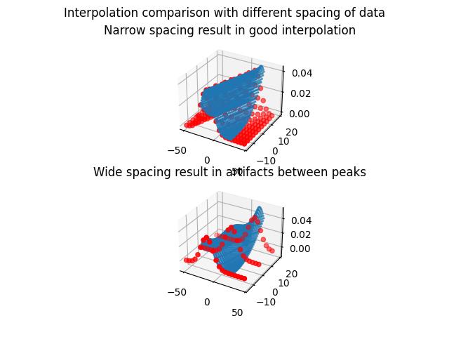
bispline(func=None, invfunc=None, tx=None, ta=None, deg=[3, 3], eps=None, addErr=False, **kwargs)¶

Weighted least-squares bivariate spline approximation for interpolation of Y at given attribute values for X values.

Uses scipy.interpolate.LSQBivariateSpline . Weights are (1/eY**2) if .eY is present.

Parameters:

kwargs: Keyword arguments The first keyword argument found as attribute is used for interpolation. E.g. conc=0.12 defines the attribute ‘conc’ to be interpolated to 0.12 Special kwargs see below.
Xarray: List of X values were to evaluate. If X not given the .X of first element are used as default.
funcnumpy ufunction or lambda: Simple function to be used on Y values before interpolation. see dataArray.polyfit
invfuncnumpy ufunction or lambda: To invert func after extrapolation again.
tx,taarray like, None, int: Strictly ordered 1-D sequences of knots coordinates for X and attribute. If None the X or attribute values are used. If integer<len(X or attribute) the respective number of equidistant points in the interval between min and max are used.
deg[int,int], optional: Degrees of the bivariate spline for X and attribute. Default is 3. If single integer given this is used for both.
epsfloat, optional: A threshold for determining the effective rank of an over-determined linear system of equations. eps should have a value between 0 and 1, the default is 1e-16.
addErrbool: If errors are present spline the error column and add it to the result.

Returns:

dataArray

Notes

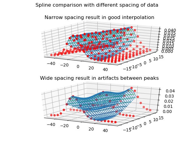
The spline interpolation results in a good approximation if the data are narrow. Around peaks values are underestimated if the data are not dense enough as the flank values are included in the spline between the maxima. See Examples.
Without peaks there should be no artifacts.
To estimate new errors for the spline data use .setColumnIndex(iy=ii,iey=None) with ii as index of errors. Then spline the errors and add these as new column.
Interpolation can not be as good as fitting with a prior known model and use this for extrapolating.

Examples

import jscatter as js
import numpy as np
import matplotlib.pyplot as plt
from mpl_toolkits.mplot3d import Axes3D
fig = plt.figure()
ax1 = fig.add_subplot(211, projection='3d')
ax2 = fig.add_subplot(212, projection='3d')

i5=js.dL([js.formel.gauss(np.r_[-50:50:5],mean,10) for mean in np.r_[-15:15.1:3]])
i5b=i5.bispline(mean=np.r_[-15:15:1],X=np.r_[-25:25:1],tx=10,ta=5)

fig.suptitle('Spline comparison with different spacing of data')
ax1.set_title("Narrow spacing result in good interpolation")
ax1.scatter3D(i5.X.flatten, np.repeat(i5.mean,[x.shape[0] for x in i5.X]), i5.Y.flatten,s=20,c='red')
ax1.scatter3D(i5b.X.flatten,np.repeat(i5b.mean,[x.shape[0] for x in i5b.X]), i5b.Y.flatten,s=2)
ax1.tricontour(i5b.X.flatten,np.repeat(i5b.mean,[x.shape[0] for x in i5b.X]), i5b.Y.flatten)

i5=js.dL([js.formel.gauss(np.r_[-50:50:5],mean,10) for mean in np.r_[-15:15.1:15]])
i5b=i5.bispline(mean=np.r_[-15:15:1],X=np.r_[-25:25:1])

ax2.set_title("Wide spacing result in artifacts between peaks")
ax2.scatter3D(i5.X.flatten, np.repeat(i5.mean,[x.shape[0] for x in i5.X]), i5.Y.flatten,s=20, c='red')
ax2.scatter3D(i5b.X.flatten,np.repeat(i5b.mean,[x.shape[0] for x in i5b.X]), i5b.Y.flatten,s=2)
ax2.tricontour(i5b.X.flatten,np.repeat(i5b.mean,[x.shape[0] for x in i5b.X]), i5b.Y.flatten)
plt.show(block=False)
# fig.savefig(js.examples.imagepath+'/bispline.jpg')

clear(/)¶: Remove all items from list.

property commonAttr¶: Returns list of attribute names existing in elements.

copy()¶

Deepcopy of dataList

To make a normal shallow copy use copy.copy

copyattr2elements(maxndim=1, exclude=['comment'])¶

Copy dataList specific attributes to all elements.

Parameters:

excludelist of str: List of attr names to exclude from show
maxndimint, default 2: Maximum dimension e.g. to prevent copy of 2d arrays like covariance matrix

Notes

Main use is for copying fit parameters.

count(value, /)¶: Return number of occurrences of value.

delete(index)¶: Delete element at index

detachErrPlot()[source]¶: Detaches ErrPlot without killing it and returns a reference to it.

dlattr(attr=None)¶

Get attribute or list of existing attribute names excluding common attributes from dataArrays.

Parameters:

attrstring: Name of dataList attribute to return. If None a list of all attribute names is returned

property dtype¶: return dtype of elements

errPlot(*args, **kwargs)[source]¶: Plot into an existing ErrPlot. See Graceplot.plot for details.

errPlotTitle(title)[source]¶: dummy

property errplot¶: Errplot handle

estimateError(method='lm', output=True)¶

Estimate error using a refined fit (method='lm') if no error is present.

As default .fit method is used with method='lm' to result in an error. A previous fit determines the starting parameters to refine the previous fit. It needs min. around 2*number_freepar function evaluations for a good $\chi^2$ minimum.

Errors are found as attributes .parname_err.

See .fit for error determination.

Parameters:

methodfit method, default ‘lm’

Fit method to use. The default ‘lm’ results in error bars.

Some other methods may not deliver errors, but can be used to restart a fit with the result of a previous fit.

outputbool

Suppress output

Examples

import jscatter as js
import numpy as np
data=js.dL(js.examples.datapath+'/iqt_1hho.dat')[::3]
diffusion=lambda t,wavevector,A,D,b:A*np.exp(-wavevector**2*D*t)+b

data.fit(model=diffusion ,
     freepar={'D':0.1,'A':1},
     fixpar={'b':0.} ,
     mapNames= {'t':'X','wavevector':'q'},method='Powell')

data.estimateError()

extend(objekt=None, index=slice(None, None, None), usecols=None, skiplines=None, replace=None, ignore='#', XYeYeX=None, delimiter=None, takeline=None, lines2parameter=None, encoding=None)¶

Reads/creates new dataArrays and appends to dataList.

See dataList for description of all keywords. If objekt is dataArray or dataList all options except XYeYeX,index are ignored.

Parameters:

objekt,index,usecols,skiplines,replace, ignore,delimiter,takeline,lines2parameteroptions: See dataArray or dataList
original doc from list
Append object to the end of the list.

extractAttribut(parName, func=None, newParName=None)¶

Extract a simpler attribute from a complex attribute in each element of dataList.

e.g. extract the mean value from a list in an attribute

Parameters:

parNamestring: Name of the parameter to process
funcfunction or lambda: A function (e.g. lambda ) that creates a new content for the parameter from the original content e.g. lambda a:np.mean(a)*5.123 The function gets the content of parameter whatever it is
newParName :string: New parname, if None old parameter is overwritten.

extrapolate(func=None, invfunc=None, xfunc=None, invxfunc=None, exfunc=None, **kwargs)¶

Inter/Extrapolated .Y values along attribute for all given X values using a polyfit.

To extrapolate along an attribute using twice a polyfit (first along X then along attribute). E.g. from a concentration series to extrapolate to concentration zero.

Parameters:

**kwargs: Keyword arguments The first keyword argument found as attribute is used for extrapolation e.g. q=0.01 attribute with values where to extrapolate to Special kwargs see below.
Xarraylike: list of X values were to evaluate
funcfunction or lambda: Function to be used in Y values before extrapolating. See Notes.
invfuncfunction or lambda: To invert function after extrapolation again.
xfuncfunction or lambda: Function to be used for X values before interpolating along X.
invxfuncfunction or lambda: To invert xfunction again.
exfuncfunction or lambda: Weight for extrapolating along X
degx,degyinteger default degx=0, degy=1: polynom degree for extrapolation in x,y If degx=0 (default) no extrapolation for X is done and values are linear interpolated.

Returns:

dataArray

Notes

funct/invfunc is used to transfer the data to a simpler smoother or polynominal form.

Think about data describing diffusion like $I=exp(-q^2Dt)$ and we want to interpolate along attribute q. If funct is np.log we interpolate on a simpler parabolic q**2 and linear in t.
Same can be done with X axis e.g. for subdiffusion $I=exp(-q^2Dt^a) \ with \ a < 1$.

Examples

# Task: Extrapolate to zero q for 3 X values for an exp decaying function.
# Here first log(Y) is used (problem linearized), then linear extrapolate and exp function used for the result.
# This is like lin extrapolation of the exponent.
#
i5.polyfit(q=0,X=[0,1,11],func=lambda y:np.log(y),invfunc=lambda y:np.exp(y),deg=1)
#
# Concentration data with conc and extrapolate to conc=0.
data.polyfit(conc=0,X=data[0].X,deg=1)
#
# Interpolate for specified X and a list of attributes. ::
i5=js.dL(js.examples.datapath+'/iqt_1hho.dat')
i5.polyfit(X=np.r_[1:5.1],q=i5.q)

filter(filterfunction=None, **kwargs)¶

Filter elements according to filterfunction and kwargs.

Parameters:

filterfunctionfunction or lambda function returning boolean: Return those items of sequence for which function(item) is true.
kwargs: Any given keyword with value is combined with filterfunction (logical AND).

Examples

i5=js.dL('exampleData/iqt_1hho.dat')
i1=i5.filter(lambda a:a.q>0.1)
i1=i5.filter(lambda a:(a.q>0.1) )
i5.filter(lambda a:(a.q>0.1) & (a.average[0]>1)).average
i5.filter(lambda a:(max(a.q*a.X)>0.1) & (a.average[0]>1))
# with kwargs
i5.filter(q=0.5,conc=1)

fit(model, freepar={}, fixpar={}, mapNames={}, method='lm', xslice=slice(None, None, None), condition=None, output=True, **kw)¶

Least square fit of model that minimizes $\chi^2$ (uses scipy.optimize methods) or Bayesian analysis.

A fit of scalar .Y values dependent on coordinates (X,Z,W) and attributes (multidimensional fitting).
Data attributes are used automatically in model if they have the same name as a parameter.
Resulting errors are 1-sigma errors as estimated from the covariance matrix diagonal for $\chi^2$ minimization or std deviation of the distribution for Bayesian inference. Errors be accessed for fit parameter D as D_err (see Fit result attributes below).
Results can be simulated with changed parameters in .modelValues, .showlastErrPlot or .simulate.

Parameters:

modelfunction or lambda

Model function, should accept arrays as input (use numpy ufunctions).

Return value should be dataArray (.Y is used) or only Y values.
Failed model evaluation should return single negative integer.

Example ( see How to build simple models ):

diffusion=lambda A,D,t,wavevector: A*np.exp(-wavevector**2*D*t)

freepardictionary

Fit parameter names with start values.

{'D':2.56,..} float, one common value for all
{'D':[1,2.3,4.5,...],..} list of float, individual parameters for independent fit.
[..] is extended with missing values equal to last given value. [2,1] -> [2,1,1,1,1,1]
It is sufficient to add [] around a float to switch between common value and independent fit values.

fixpardictionary

Fixed parameters (see freepar for syntax). Overwrites data attributes with same name.

mapNamesdictionary

Map parameter names from model to attribute names in data e.g. {‘t’:’X’,’wavevector’:’q’,}

method‘lm’, ‘trf’, ‘dogbox’, ‘Nelder-Mead’, ‘bayes’, ‘differential_evolution’, ‘BFGS’,

or scipy.optimize.minimize methods

Type of solver for minimization

See later fit methods for usage hints and a speed comparison. Fastest are ‘lm’, “trf”, “dogbox”.

‘lm’ (default) and what you typically expect for fitting and should be first choice without bounds. It is a wrapper around MINPACK’s lmdif and lmder algorithms which are a modification of the Levenberg-Marquardt algorithm. Returns errors. With limits ‘trf’ is used.
‘trf’ (default with limits) trust-region reflective algorithm, similar to ‘lm’ but with bounds. Returns errors.
‘dogbox’ a trust-region algorithm, but considers rectangular trust regions. Returns errors.
‘Nelder-Mead’ allows optimization of integer variables. Additionally it is sometime more robust if gradient methods (like above) break early or stick in a local minimum. NO errors.
‘BFGS’ quasi-Newton method of Broyden, Fletcher, Goldfarb, and Shanno. Uses the first derivatives only. Returns errors.
‘bayes’ uses Bayesian inference for modeling and the MCMC algorithms for sampling (we use emcee). Requires a larger amount of function evaluations but returns errors from Bayesian statistical analysis. Check additional description and parameters below. Needs limits, which are set as for differential_evolution. See getBayesSampler() with example. The model should not use multiprocessing as ‘bayes’ uses this already. The prior can be changed using the additional parameter ln_prior.
‘differential_evolution’ is a stochastic population based method that is useful for global optimization problems. Needs bounds for all parameters as used from .setlimit.
- If no bounds are set bounds are generated automatic around start value x0 as [x0/10**0.5,x0*10**0.5].
- The optional workers argument allows parallel processing in a pool of workers. workers=-1 uses all cpus, otherwise the number of cpus (default all).
NO errors.
All methods use bounds set by .setlimits to allow bounds as described there. For ‘trf’, ‘dogbox’ the bounds implemented in the method are used taken from setlimit soft bounds.
For additonal options passed to scipy.optimize least_square (‘lm’, ‘trf’, ‘dogbox’) or minimize (others) see scipy.optimize. For some methods the Jacobian is required.

xsliceslice object

Select datapoints to include by slicing

xslice=slice(2,-3,2)       To skip first 2,last 3 and take each second.

conditionfunction or lambda

A function to determine which datapoints to include.

The function should evaluate to boolean with dataArray as input and combines with xslice used on full set (first xslice then the condition is used)

local operation on numpy arrays as “&”(and), “|”(or), “^”(xor)

sel = lambda a:(a.X>1) & (a.Y<1)
sel = lambda a:(a.X>1) & (a.X<100)
sel = lambda a: a.X>a.q * a.X
Rg = 4 # nm
gunier = lambda a: a.X**2*Rg**2/3 < 1

Use as condition = sel or condition=lambda a:(a.X>1) & (a.Y<1)

output‘last’,’best’, False, default True

By default write some text messages (fit progress).

‘last’ return lastfit and text messages
‘best’ return best (parameters,errors) and text messages
False : No printed output.

debug1,2,3,int

Debug modus returns:

1 simulation mode: parameters sent to model, errPlot and modelValues without fitting.
2 Free and fixed parameters but not mappedNames.
3 Fitparameters in modelValues as dict to call model as model(**kwargs) with mappedNames.
4 Prints parameters sent to model and returns the output of model without fitting.
>4 -> 1

kwadditional keyword arguments

Additional kw forwarded to fit method as given in scipy.optimize for least_square or minimize or emcee.

See simple additional kwargs

Returns:

By default no return value.

Final results with errors are in .lastfit
Fitparameters are additional in dataList object as .parname and corresponding errors as .parname_err.
If the fit fails an exception is raised and last parameters are printed.
!!_These_are_NOT_a_valid_fit_result_!!.

Notes

For $\mathbf{\chi^2 minimization}$ the unbiased estimate

\[\chi^2 = \frac{1}{n-p} \sum_i \frac{[X_i-f(X_i,a)]^2}{\sigma_i^2}\]

with number of datapoints $n$, number of parameters $p$ and function $f(X_i,a)$ dependent on parameters $a_i$ is minimized. Differences are weighted by measurement errors $\sigma_i^2$. Methods from scipy.optimize are used.

For Bayesian analysis (‘bayes’) the log probability $\ln\,p(y\,|\,x,\sigma,a) + log(p(a_i))$ is maximized with the log likelihood $ln (p(y\,|\,x,\sigma,a))$

\[\ln\,p(y\,|\,x,\sigma,a) = -\frac{1}{2} \sum_i \left[\frac{(X_i-f(X_i,a))^2}{\sigma_i^2} + \ln \left ( 2\pi\,\sigma_i^2 \right )\right]`\]

and the prior $p(a_i)$. By default an uniform (so-called “uninformative”) prior is used

\[\begin{split}log(p(a_i)) = \left\{ \begin{array}{ll} 0 & \mbox{if $a_i$ in limits};\\ -inf & \mbox{otherwise}.\end{array} \right.\end{split}\]

which can be changed using the parameter ln_prior to a more informative prior.

See emcee for details how this works and further analysis or options.
For $\mathbf{\chi^2}$ minimization the resulting parameter errors are 1-sigma errors as determined from the covariance matrix (see [1]). This holds under some (and some more) assumptions :
- We have a well-behaved likelihood function (same as in ‘bayes’) which is asymptotically Gaussian near its maximum (equal to minimum in $\chi^2$).
- The error estimate is reasonable (1-sigma measurement errors in data).
- The model is the correct model.
- The model parameters are linear close to the $\chi^2$ minimum.
These reasons might also limit the best $\chi^2$ values reached in a fit (e.g. it reaches only 2 instead of 1) if a simplified model is used.

Practically, the resulting parameter error is (roughly) independent of the absolute value of errors in the data as long as the relative contributions are well represented. Thus scaling of the errors by a factor leads to same 1-sigma error, respectively the 1-sigma errors are independent of the absolute error scale. Please try this by modifying the examples given, it can be proved analytically.
For Bayesian estimations (‘bayes’) errors are determined from the likelihood and represent the standard deviation of the mean in the real likelyhood. (see [1] 3.4 ).

By default an uninfomative prior within set limits is used. This can be changed passing a log_prior function to the parameter ln_prior which contains any prior information about the parameters (NOT the data). This might be e.g. that some parameters are itself distributed like a Gaussian around a mean or their differences. The log_prior function gets as parameters all freepar and fixpar arrays (but not the .X values from data). If likelyhood and prior are correctly weighted ( for each $\mathbf{\chi^2}$ is 1 ) both contribute equally to the probability. An example with a prior is given in Bayesian inference for fitting.

A sufficient requirement for the here used methods from emcee is that the sample number $N > tolerance * \tau_f$ with the autocorrelation time $\tau_f$ and the tolerance =50, which means having just enough samples to get reasonable statistics. The fit method tries in steps of bayesnsteps to determine $\tau_f$ and proceeds until the requirement is satisfied. tolerance is by default =50 but can be reduced for testing before a production run. Also, nwalkers (default 2*number of parameters) can be changed. $2\tau_f$ is discarded from the chain for analysis to remove bias. See getBayesSampler() to get the emcee sampler and for example usage.

The disadvantage of ‘bayes’ is that simple problems need a quite large number of function evaluations. E.g. the below comparison needs around 10000 evaluations for a single dataArray compard to around 30 for method ‘lm’ for the full dataList. More complex models that need longer than 1s to evaluate need hours to days to finish. For single datasets with fast evaluated functions ‘bayes’ works reasonable well. For these reasons ‘bayes’ works by default with a pool of workers (multiprocessing) which wins largely on a multicore machine with more than 16 cpus and is not well for a notebook.

For good data with small errors ‘bayes’ should not be used as there is no advantage compared to e.g. ‘lm’ (‘lm’ results in good error estimate in this case). If your data and model have trouble to find a $\chi^2$ minimum or find often local minima give ‘bayes’ a try. After testing (small tolerance) the sampling might run for longer times if needed. The samples can be accessed after the fitting to examine the results. See getBayesSampler().

My personal impression is that if you have a chance to improve your measurement do this and use ‘lm’ or ‘trp’ before spending the time on long ‘bayes’ estimation. For unique data (your spectral analysis of Halley’s comet) one can improve analysis using ‘bayes’.
If data errors exist ($\sigma_i$ = .eY) and are not zero, the error weighted $\chi^2$ is minimized (or respective weighted likelihood is maximized). Without error (or with single errors equal zero) unweighted values respective equal weights are used.
- Using unweighted error means basically equal weight as $\sigma_i^2 =1$ in $\chi^2$ above. This might lead to biased results.
- If no errors are directly available it is useful (or a better error estimate than equal weights) to introduce a weight that represents the statistical nature of the measurement (at least the dominating term in error propagation).
  - equal errors $\sigma_i \propto const$
  - equal relative error $\sigma_i \propto .Y$
  - statistical $\sigma_i \propto .Y^{0.5}$ e.g. Poisson statistics on neutron/Xray detector.
  - with bgr $\sigma_i \propto .Y+b$
  - any other $\sigma_i \propto f(.X,.Y,...)$
  To use one or the other a column needs to be added with the respective values and use .setColumnIndex(iey=…) to mark it as error column .eY . Set values as e.g. data.eY=0.01*data.Y for equal relative errors.
The concept of dataLists is to use data attributes as fixed parameters for the fit (multidimensional fit). This is realized by using data attributes with same name as fixed parameters if not given explicitly in freepar or fixpar.
Fit parameters can be set equal for all elements 'par':1 or independent 'par':[1] just by writing the start value as a single float or as a list of float. The same for fixed parameters.
Changing between free and fixed parameters is easily done by moving 'par':[1] between freepar and fixpar.
Limits for parameters can be set prior to the fit as .setlimit(D=[1,4,0,10]). The first two numbers (min,max) are softlimits (increase $\chi^2$) and second are hardlimits to avoid extreme values. (hard set to these values if outside interval and increasing $\chi^2$).
The change of parameters can be simulated by .modelValues(D=3) which overrides attributes and fit parameters.
.makeErrPlot() creates an errorplot with residuals prior to the fit for intermediate output.
The last errPlot can be recreated after the fit with .showlastErrPlot().
The simulated data can be shown in errPlot with .showlastErrPlot(D=3).

Each dataArray in a dataList can be fit individually (same model function) like this

# see Examples for dataList creation
data[3].fit(model,freepar,fixpar,.....)
# or
for dat in data:
    dat.fit(model,freepar,fixpar,.....)

Most important additional kwargs for ‘least_square’ methods ‘lm’, ‘trf’, ‘dogbox’

arguments passed to least_squares (see scipy.optimize.least_square)
ftol          default  1.e-8      Relative error desired in the sum of squares (also tol accepted)
xtol          default  1.e-8      Relative error desired in the approximate best parameters.
gtol          default  1.e-8      Tolerance for termination by the norm of the gradient.
max_nfev      default ~100*N(*N 'lm')   Maximum model evaluations (also maxiter accepted)
diff_step     default None,       relative step size = x*diff_step for finite differences
                                  approx. of the Jacobian.

Most important additional kwargs for ‘minimize’ methods ‘Nelder-Mead’, ‘BFGS’,…

arguments passed to minimize
tol           tolerance for termination. Depends on algorithm. (also max_nfev excepted)
maxiter       maximum model evaluations (also max_nfev accepted)

Fit result attributes

# exda are fitted example data
exda.D                    freepar 'D' ; same for fixpar but no error.
                          use exda.lastfit.attr to see all attributes of model
exda.D_err                1-sigma error of freepar 'D'
# full result in lastfit
exda.lastfit.X            X values in fit model
exda.lastfit.Y            Y values in fit model
exda.lastfit[i].D         free parameter D result in best fit
exda.lastfit[i].D_err     error of free parameter D as 1-sigma error from diagonal in covariance matrix.
exda.lastfit.chi2         chi2 = sum(((.Y-model(.X,best))/.eY)**2)/dof; should be around 1 with proper weight.
exda.lastfit.cov          covariance matrix = hessian**-1 * chi2
exda.lastfit.dof          degrees of freedom = len(y)-len(best)
exda.lastfit.func_name    name of used model
exda.lastfit.func_code    where to find code of used model

References

About error estimate from covariance Matrix M with the Fischer matrix $F$ (like gradien methods)

\[cM_{i,j}=(\frac{\partial^2 log(F) }{ \partial x_i\partial x_j})^{-1} .\]

[1] (1,2)

https://arxiv.org/pdf/1009.2755.pdf

Examples

How to make a model: The model function gets .X (.Z, .W, .eY, ....) as ndarray and parameters (from attributes and freepar and fixpar) as scalar input. It should return a ndarray as output (only .Y values) or dataArray (.Y is used automatically). Therefore, it is advised to use numpy ufunctions in the model. Instead of math.sin use numpy.sin, which is achieved by import numpy as np and use np.sin see https://numpy.org/doc/stable/reference/ufuncs.html#available-ufuncs

See How to build simple models and How to build a more complex model

A bunch of examples can be found in formel.py, formfactor.py, stucturefactor.py.

Basic examples with synthetic data.

Usually data are loaded from a file. For the following also see 1D fits with attributes and 2D fitting .

An error plot with residuals can be created for intermediate output. The model is here a lambda function

import jscatter as js
import numpy as np
data=js.dL(js.examples.datapath+'/iqt_1hho.dat')
diffusion=lambda t,wavevector,A,D,b:A*np.exp(-wavevector**2*D*t)+b
data.setlimit(D=(0,2))               # set a limit for diffusion values
data.makeErrPlot()                   # create errorplot which is updated
data.fit(model=diffusion ,
     freepar={'D':0.1,               # one value for all (as a first try)
              'A':[1,2,3]},          # extended to [1,2,3,3,3,3,...3] independent parameters
     fixpar={'b':0.} ,               # fixed parameters here, [1,2,3] possible
     mapNames= {'t':'X',             # maps time t of the model as .X column for the fit.
                'wavevector':'q'},   # and map model parameter 'wavevector' to data attribute .q
     condition=lambda a:(a.Y>0.1) )  # set a condition

Fit sine to simulated data. The model is inline lambda function.

import jscatter as js
import numpy as np
x=np.r_[0:10:0.1]
data=js.dA(np.c_[x,np.sin(x)+0.2*np.random.randn(len(x)),x*0+0.2].T)           # simulate data with error
data.fit(lambda x,A,a,B:A*np.sin(a*x)+B,{'A':1.2,'a':1.2,'B':0},{},{'x':'X'})  # fit data
data.showlastErrPlot()                                                         # show fit
print(  data.A,data.A_err)                                                        # access A and error

Fit sine to simulated data using an attribute in data with same name

x=np.r_[0:10:0.1]
data=js.dA(np.c_[x,1.234*np.sin(x)+0.1*np.random.randn(len(x)),x*0+0.1].T)     # create data
data.A=1.234                                                                   # add attribute
data.makeErrPlot()                                                             # makes errorPlot prior to fit
data.fit(lambda x,A,a,B:A*np.sin(a*x)+B,{'a':1.2,'B':0},{},{'x':'X'})          # fit using .A

Fit sine to simulated data using an attribute in data with different name and fixed B

x=np.r_[0:10:0.1]
data=js.dA(np.c_[x,1.234*np.sin(x)+0.1*np.random.randn(len(x)),x*0+0.1].T)       # create data
data.dd=1.234                                                                    # add attribute
data.fit(lambda x,A,a,B:A*np.sin(a*x)+B,{'a':1.2,},{'B':0},{'x':'X','A':'dd'})   # fit data
data.showlastErrPlot()                                                           # show fit

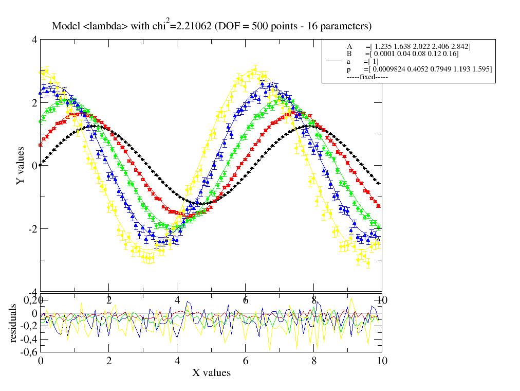
Fit sine to simulated dataList using an attribute in data with different name and fixed B from data. first one common parameter then as parameter list in [].

import jscatter as js
import numpy as np
x=np.r_[0:10:0.1]
data=js.dL()
ef=0.1  # increase this to increase error bars of final result
for ff in [0.001,0.4,0.8,1.2,1.6]:                                                      # create data
    data.append( js.dA(np.c_[x,(1.234+ff)*np.sin(x+ff)+ef*ff*np.random.randn(len(x)),x*0+ef*ff].T) )
    data[-1].B=0.2*ff/2                                                                 # add attributes
#
# fit with a single parameter for all data, obviously wrong result
data.fit(lambda x,A,a,B,p:A*np.sin(a*x+p)+B,{'a':1.2,'p':0,'A':1.2},{},{'x':'X'})
data.showlastErrPlot()                                                                 # show fit
#
# now allowing multiple p,A,B as indicated by the list starting value
data.fit(lambda x,A,a,B,p:A*np.sin(a*x+p)+B,{'a':1.2,'p':[0],'B':[0,0.1],'A':[1]},{},{'x':'X'})
#data.savelastErrPlot(js.examples.imagepath+'/4sinErrPlot.jpg')
# plot p against A , just as demonstration
p=js.grace()
p.plot(data.A,data.p,data.p_err)

2D/3D/xD fit for scalar Y

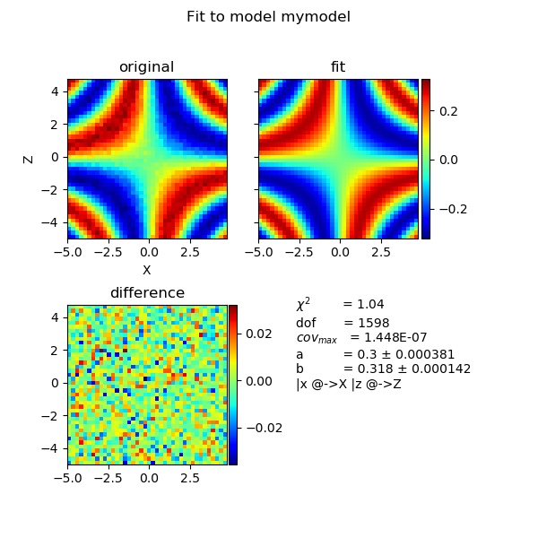
For 2D fit we calc Y values from X,Z coordinates, for 3D fits we use X,Z,W coordinates. For 2D plotting of the result we need data in X,Z,Y column format. This can be combined with attribute dependence to result in higher dimensional fits.

import jscatter as js
import numpy as np
#
# create 2D data with X,Z axes and Y values as Y=f(X,Z)
x,z=np.mgrid[-5:5:0.25,-5:5:0.25]
xyz=js.dA(np.c_[x.flatten(),
                z.flatten(),
                0.3*np.sin(x*z/np.pi).flatten()+0.01*np.random.randn(len(x.flatten())),
                0.01*np.ones_like(x).flatten() ].T)
# set columns where to find X,Y,Z )
xyz.setColumnIndex(ix=0,iz=1,iy=2,iey=3)
#
def mymodel(x,z,a,b):
     return a*np.sin(b*x*z)
xyz.fit(mymodel,{'a':1,'b':1/3.},{},{'x':'X','z':'Z'})
# inspect the result
fig = js.mpl.showlastErrPlot2D(xyz)
#fig.savefig(js.examples.imagepath+'/2dfit.jpg')

Fit for vector valued results

Vectors (multidimensional results or vector Y values) like a vector field are fitted by minimizing a specific norm (L2 or other) of the difference between measured vectors and model vectors. Doing this the fit is reduced to a scalar fit as above.

Comparison of fit methods

import numpy as np
import jscatter as js
diffusion=lambda A,D,t,elastic,wavevector=0:A*np.exp(-wavevector**2*D*t)+elastic

i5=js.dL(js.examples.datapath+'/iqt_1hho.dat')
i5.makeErrPlot(title='diffusion model residual plot')

# default
i5.fit(model=diffusion,freepar={'D':0.2,'A':1}, fixpar={'elastic':0.0},
       mapNames= {'t':'X','wavevector':'q'},
       condition=lambda a:a.X>0.01, method='lm')
# 22 evaluations; error YES -> 'lm'
# with D=[0.2] => 130 evaluations and chi2 = 0.992

i5.fit(model=diffusion,freepar={'D':0.2,'A':1}, fixpar={'elastic':0.0},
       mapNames= {'t':'X','wavevector':'q'},
       condition=lambda a:a.X>0.01, method='trf')
# 22 evaluations; error YES
# with D=[0.2] => 145 evaluations and chi2 = 0.992

i5.fit(model=diffusion,freepar={'D':0.2,'A':1}, fixpar={'elastic':0.0},
       mapNames= {'t':'X','wavevector':'q'},
       condition=lambda a:a.X>0.01, method='dogbox')
# 22 evaluations; error YES
# with D=[0.2] => 145 evaluations and chi2 = 0.992

i5.fit(model=diffusion,freepar={'D':0.2,'A':1}, fixpar={'elastic':0.0},
       mapNames= {'t':'X','wavevector':'q'},
       condition=lambda a:a.X>0.01 ,method='Nelder-Mead' )
# 72 evaluations, error NO

i5.fit(model=diffusion,freepar={'D':0.2,'A':1}, fixpar={'elastic':0.0},
       mapNames= {'t':'X','wavevector':'q'},
       condition=lambda a:a.X>0.01, method='differential_evolution', workers=-1)
# >400 evaluations, error NO ; needs >20000 evaluations using D=[0.2]
# profits strongly from worker>1 (-1 = all) to use multiple processes (not on Windows)
# use only with low number of parameters and polish result with methods yielding errors.

i5.fit(model=diffusion,freepar={'D':0.2,'A':1}, fixpar={'elastic':0.0},
       mapNames= {'t':'X','wavevector':'q'},
       condition=lambda a:a.X>0.01, method='bayes', tolerance=50, bayesnsteps=1000)
# >10000 evaluations; error YES
# tolerance should be >= 50 not smaller
# The full dataset takes some time (for testing -> tolerance=20 or i6=i5[::3])
# use only with low number of parameters and polish result when you really need it

i5.fit(model=diffusion,freepar={'D':0.2,'A':1}, fixpar={'elastic':0.0},
       mapNames= {'t':'X','wavevector':'q'},
       condition=lambda a:a.X>0.01 ,method='Powell' )
# 121 evaluations; error NO

i5.fit(model=diffusion,freepar={'D':0.2,'A':1}, fixpar={'elastic':0.0},
       mapNames= {'t':'X','wavevector':'q'},
       condition=lambda a:a.X>0.01 ,method='SLSQP' )
# 37 evaluations, error NO

i5.fit(model=diffusion,freepar={'D':0.2,'A':1}, fixpar={'elastic':0.0},
       mapNames= {'t':'X','wavevector':'q'},
       condition=lambda a:a.X>0.01 ,method='BFGS' )
# 52 evaluations, error YES
# with D=[0.2] => 931 evaluations and chi2 = 0.992

i5.fit(model=diffusion,freepar={'D':0.2,'A':1}, fixpar={'elastic':0.0},
       mapNames= {'t':'X','wavevector':'q'},
       condition=lambda a:a.X>0.01 ,method='COBYLA' )
# 269 evaluations, error NO

getBayesSampler()¶

Returns Bayes sampler after Bayesian fit for further analysis.

First do a fit with method=’bayes’ then the sampler can be retrieved.

Returns:

emcee sampler

Examples

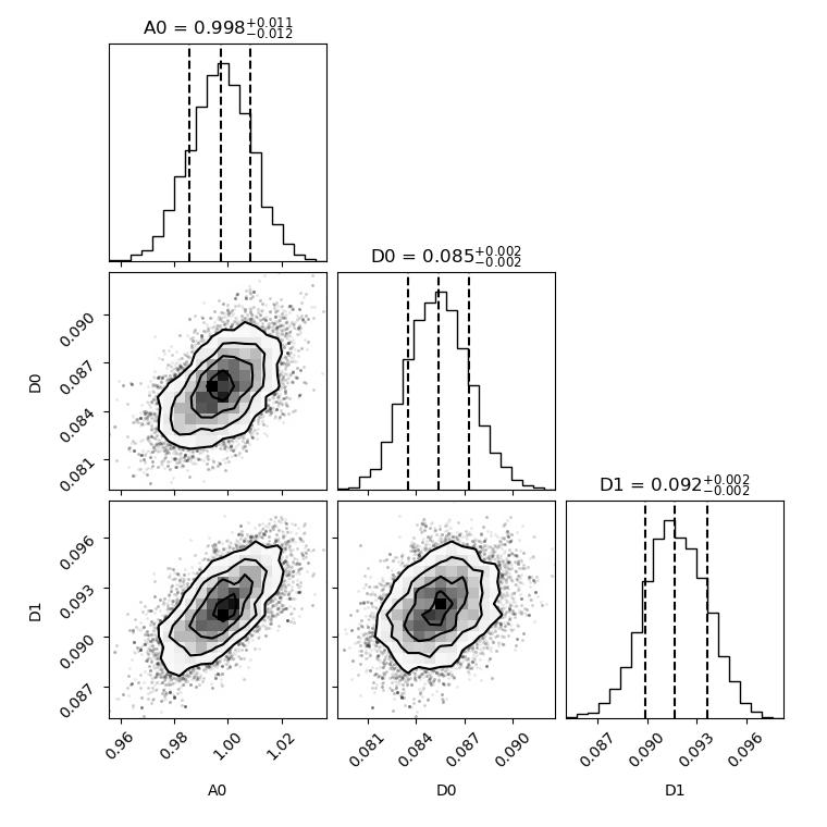
Access the chain and make a corner plot

First install corner for the corner plot pip install corner See https://corner.readthedocs.io/en/latest/index.html

import jscatter as js
import numpy as np
import matplotlib.pyplot as plt
import corner

diffusion=lambda A,D,t,elastic,wavevector=0:A*np.exp(-wavevector**2*D*t)+elastic

i5=js.dL(js.examples.datapath+'/iqt_1hho.dat')[[5,6]]
i5.makeErrPlot(title='diffusion model residual plot')

# get better starting values
i5.fit(model=diffusion,freepar={'D':[0.2],'A':1}, fixpar={'elastic':0.0},
        mapNames= {'t':'X','wavevector':'q'},
        condition=lambda a:a.X>0.01, method='lm')

# do the emcee Bayes fit
i5.fit(model=diffusion,freepar={'D':i5.D,'A':i5.A}, fixpar={'elastic':0.0},
        mapNames= {'t':'X','wavevector':'q'},
        condition=lambda a:a.X<80, method='bayes', tolerance=50, bayesnsteps=1000)

# get sampler chain and examine results removing burn in time 2*tau
tau = i5.getBayesSampler().get_autocorr_time(tol=50)
flat_samples = i5.getBayesSampler().get_chain(discard=int(2*tau.max()), thin=1, flat=True)
labels = i5.getBayesSampler().parlabels

plt.ion()
fig = corner.corner(flat_samples, labels=labels,quantiles=[0.16, 0.5, 0.84],show_titles=True,title_fmt='.3f')
plt.show()
# fig.savefig(js.examples.imagepath+'/bayescorner.jpg')

getChi2Trace()¶

Get the trace of function evaluations after a fit.

Maybee useful in ‘differential evolution’ to get last ensembles or to see fit convergence. Or to restart fits that break because of other conditions.

Works only if fit method does not use multiprocessing like e.g. ‘bayes’. Multiprocessing in the model is allowed.

Returns:

array with [index, chi2, par1, par2,…]

Examples

import jscatter as js
import numpy as np

data=js.dA(js.examples.datapath+'/exampledata0.dat')

def parabola(q,a,b,c):
   return (q-a)**2+b*q+c
par = {'a':2,'b':4}
data.fit( model=parabola ,freepar=par, fixpar={'c':-20}, mapNames={'q':'X'})

trace = data.getChi2Trace()

# to restart a fit or simulate the model values with the last parameters
lastpar = {k.strip():v for k,v in zip(trace.columnname.split(';')[2:], trace.array[2:,-1])}

data.fit( model=parabola ,freepar=lastpar, fixpar={'c':-20}, mapNames={'q':'X'})

getfromcomment(attrname, convert=None, ignorecase=False)¶

Extract a non number parameter from comment with attrname in front

If multiple names start with parname first one is used. Used comment line is deleted from comments

Parameters:

attrnamestring without spaces

Name of the parameter in first place.

convertfunction

Function to convert the remainder of the line to the desired attribut value. E.g.

# line "Frequency - 3.141 MHz "
.getfromcomment('Frequency',convert=lambda a: float(a.split()[1]))

ignorecasebool

Ignore case of attrname.

Notes

A more complex example with unit conversion

f={'GHz':1e9,'MHz':1e6,'KHz':1e3,'Hz':1}
# line "Frequency - 3.141 MHz "
.getfromcomment('Frequency',convert=lambda a: float(a.split()[1]) * f.get(a.split()[2],1))

property hasConstrain¶: Return list with defined constrained source code.

property hasLimit¶

Return existing limits

without limits returns None

property has_limit¶

Return existing limits

without limits returns None

index(value, start=0, stop=-1)¶

original doc from list Return first index of value.

Raises ValueError if the value is not present.

insert(i, objekt=None, index=0, usecols=None, skiplines=None, replace=None, ignore='#', XYeYeX=None, delimiter=None, takeline=None, lines2parameter=None, encoding=None)¶

Reads/creates new dataArrays and inserts in dataList.

If objekt is dataArray or dataList all options except XYeYeX,index are ignored.

Parameters:

iint, default 0

Position where to insert.

objekt,index,usecols,skiplines,replace,ignore,delimiter,takeline,lines2parameteroptions: See dataArray or dataList

original doc from list

Insert object before index.

interpolate(func=None, invfunc=None, deg=1, col='Y', **kwargs)¶

2D interpolation of .Y values at new attribute and .X values using piecewise spline interpolation.

Uses twice an interpolation (first along .X then along attribute). Common and equal attributes are copied automatically to the interpolated dataList.

Parameters:

**kwargskeyword arguments with float or array-like values.: The first keyword argument found as attribute is used for interpolation. E.g. conc=0.12 defines the attribute ‘conc’ to be interpolated to 0.12
Xarray: List of new X values were to evaluate (linear interpolation for X). If X < or > self.X the corresponding min/max border is used. If X not given the .X of first dataList element are used as default.
colindex or char for column, default ‘Y’: Which column to interpolate. Can be column index
funcfunction or lambda: Function to be used on Y values before interpolation. See dataArray.polyfit.
invfuncfunction or lambda: To invert func after extrapolation again.
deg[int,int], optional: Degrees of the spline for X and attribute. Default is 1 for linear. If single integer given this is used for both. Outliers result in Nan. See scipy.interpolate.interp1d for more options.

Returns:

dataArray

Notes

Values outside the range of .X, .Y are extrapolated. Values outside the range of the interpolated attribute are also extrapolated. Both migth produce strange result if to far away.
This interpolation results in a good approximation if the data are narrow. Around peaks values are underestimated if the data are not dense enough. See Examples.
To estimate new errors for the spline data use .setColumnIndex(iy=ii,iey=None) with ii as index of errors. Then spline the errors and add these as new column.
Interpolation can not be as good as fitting with a prior known model and use this for extrapolating.

Examples

import jscatter as js
import numpy as np
import matplotlib.pyplot as plt
from mpl_toolkits.mplot3d import Axes3D
fig = plt.figure()
ax1 = fig.add_subplot(211, projection='3d')
ax2 = fig.add_subplot(212, projection='3d')
# try different kinds of polynominal degree
deg=2
# generate some data (gaussian with mean)
i5=js.dL([js.formel.gauss(np.r_[-50:50:5],mean,10) for mean in np.r_[-15:15.1:3]])
# interpolate for several new mean values and new X values
i5b=i5.interpolate(mean=np.r_[-15:20:1],X=np.r_[-25:25:1],deg=deg)
#
fig.suptitle('Interpolation comparison with different spacing of data')
ax1.set_title("Narrow spacing result in good interpolation")
ax1.scatter3D(i5.X.flatten, np.repeat(i5.mean,[x.shape[0] for x in i5.X]), i5.Y.flatten,s=20,c='red')
ax1.scatter3D(i5b.X.flatten,np.repeat(i5b.mean,[x.shape[0] for x in i5b.X]), i5b.Y.flatten,s=2)
ax1.tricontour(i5b.X.flatten,np.repeat(i5b.mean,[x.shape[0] for x in i5b.X]), i5b.Y.flatten)
#
i5=js.dL([js.formel.gauss(np.r_[-50:50:5],mean,10) for mean in np.r_[-15:15.1:15]])
i5b=i5.interpolate(mean=np.r_[-15:20:1],X=np.r_[-25:25:1],deg=deg)
#
ax2.set_title("Wide spacing result in artifacts between peaks")
ax2.scatter3D(i5.X.flatten, np.repeat(i5.mean,[x.shape[0] for x in i5.X]), i5.Y.flatten,s=20,c='red')
ax2.scatter3D(i5b.X.flatten,np.repeat(i5b.mean,[x.shape[0] for x in i5b.X]), i5b.Y.flatten,s=2)
ax2.tricontour(i5b.X.flatten,np.repeat(i5b.mean,[x.shape[0] for x in i5b.X]), i5b.Y.flatten)
plt.show(block=False)

killErrPlot(filename=None)[source]¶

Kills ErrPlot

If filename given the plot is saved.

makeErrPlot(title=None, **kwargs)[source]¶

Creates a GracePlot for intermediate output from fit with residuals.

ErrPlot is updated only if consecutive steps need more than 2 seconds. The plot can be accessed later as .errplot .

Parameters:

titlestring

Title of plot.

residualsstring

Plot type of residuals (=y-f(x,…)).

‘absolut’ or ‘a’ absolute residuals
‘relative’ or ‘r’ relative =residuals/y
‘x2’ or ‘x’ residuals/eY with chi2 =sum((residuals/eY)**2)

showfixparboolean default: True

Show the fixed parameters in errplot.

yscale,xscale‘n’,’l’ for ‘normal’, ‘logarithmic’

Y scale, log or normal (linear)

fitlinecolorint, [int,int,int]

Color for fit lines (or line style as in plot). If not given same color as data.

legpos‘ll’, ‘ur’, ‘ul’, ‘lr’, [rx,ry]

Legend position shortcut in viewport coordinates. Shortcuts for lower left, upper right, upper left, lower right or relative viewport coordinates as [0.2,0.2].

headlessbool, ‘agr’, ‘png’, ‘jpg’, ‘svg’, ‘pnm’, ‘pdf’

Use errPlot in headless mode (NO-Gui). True saves to lastErrPlot.agr with regular updates (all 2 seconds). A file type changes to specified file type as printed.

size[float, float]

Plot size in inch.

Examples

ErrPlot with fitted data (points), model function (lines) and the difference between both in an additional plot to highlight differences.

makeNewErrPlot(**kwargs)[source]¶

Creates a NEW ErrPlot without destroying the last. See makeErrPlot for details.

Parameters:

**kwargs: Keyword arguments passed to makeErrPlot.

merge(indices, isort=None, missing=None)¶

Merges elements of dataList.

The merged dataArray is stored in the lowest indices. Others are removed.

Parameters:

indicesinteger,’all’

List of indices to merge ‘all’ merges all elements into one.

isortinteger, default None

Sort after merge along specified column e.g.isort=’X’, ‘Y’, or 0,1,2

missingNone, ‘error’, ‘drop’, ‘skip’, ‘first’ default=None

Determines how to deal with missing attributes.

Insert None
Raise AttributeError
‘drop’ attribute value for missing
‘skip’ attribute for all
Use ‘first’ value

Notes

Attributes are copied as lists in the merged dataArray.

mergeAttribut(parName, limit=None, isort=None, func=<function mean>)¶

Merges elements of dataList if attribute values are closer than limit (in place).

If attribute is list the average is taken for comparison. For special needs create new parameter and merge along this.

Parameters:

parNamestring: name of a parameter
limitfloat: The relative limit value. If limit is None limit is determined as standard deviation of sorted differences as limit=np.std(np.array(data.q[:-1])-np.array(data.q[1:]))/np.mean(np.array(self.q)
isort‘X’, ‘Y’ or 0,1,2…, default None: Column for sort.
funcfunction or lambda, default np.mean: A function to create a new value for parameter. see extractAttribut stored as .parName+str(func.func_name)

Examples

i5=js.dL('exampleData/iqt_1hho.dat')
i5.mergeAttribut('q',0.1)
# use qmean instead of q or calc the new value
print(i5.qmean)

modelValues(**kwargs)¶

Get modelValues allowing simulation with changed parameters.

Model parameters are used from dataArray attributes or last fit parameters after a fit. Given arguments overwrite parameters and attributes to simulate modelValues e.g. to extend X range.

Parameters:

**kwargsparname=value: Overwrite parname with value in the dataList attributes or fit results e.g. to extend the parameter range or simulate changed parameters.
debuginternal usage documented for completes: dictionary passed to model to allow calling model as model(**kwargs) for debugging

Returns:

dataList of modelValues with parameters as attributes.

Notes

Example: extend time range

data=js.dL('iqt_1hho.dat')
diffusion=lambda A,D,t,wavevector: A*np.exp(-wavevector**2*D*t)
data.fit(diffusion,{'D':[2],'amplitude':[1]},{},{'t':'X'})    # do fit
# overwrite t to extend range
newmodelvalues=data.modelValues(t=numpy.r_[0:100])   #with more t

Example: 1-sigma interval for D

import jscatter as js
import numpy as np
data=js.dL(js.examples.datapath + '/iqt_1hho.dat')
diffusion=lambda A,D,t,q: A*np.exp(-q**2*D*t)
data.fit(diffusion,{'D':[0.1],'A':[1]},{},{'t':'X'})    # do fit
# add errors of D for confidence limits
upper=data.modelValues(D=data.D+data.D_err)
lower=data.modelValues(D=data.D-data.D_err)
data.showlastErrPlot()
data.errPlot(upper,sy=0,li=[2,1,1])
data.errPlot(lower,sy=0,li=[2,1,1])

nakedCopy()¶: Returns copy without attributes, thus only the data.

property names¶: List of element names.

polyfit(func=None, invfunc=None, xfunc=None, invxfunc=None, exfunc=None, **kwargs)¶

Inter/Extrapolated .Y values along attribute for all given X values using a polyfit.

To extrapolate along an attribute using twice a polyfit (first along X then along attribute). E.g. from a concentration series to extrapolate to concentration zero.

Parameters:

**kwargs: Keyword arguments The first keyword argument found as attribute is used for extrapolation e.g. q=0.01 attribute with values where to extrapolate to Special kwargs see below.
Xarraylike: list of X values were to evaluate
funcfunction or lambda: Function to be used in Y values before extrapolating. See Notes.
invfuncfunction or lambda: To invert function after extrapolation again.
xfuncfunction or lambda: Function to be used for X values before interpolating along X.
invxfuncfunction or lambda: To invert xfunction again.
exfuncfunction or lambda: Weight for extrapolating along X
degx,degyinteger default degx=0, degy=1: polynom degree for extrapolation in x,y If degx=0 (default) no extrapolation for X is done and values are linear interpolated.

Returns:

dataArray

Notes

funct/invfunc is used to transfer the data to a simpler smoother or polynominal form.

Think about data describing diffusion like $I=exp(-q^2Dt)$ and we want to interpolate along attribute q. If funct is np.log we interpolate on a simpler parabolic q**2 and linear in t.
Same can be done with X axis e.g. for subdiffusion $I=exp(-q^2Dt^a) \ with \ a < 1$.

Examples

# Task: Extrapolate to zero q for 3 X values for an exp decaying function.
# Here first log(Y) is used (problem linearized), then linear extrapolate and exp function used for the result.
# This is like lin extrapolation of the exponent.
#
i5.polyfit(q=0,X=[0,1,11],func=lambda y:np.log(y),invfunc=lambda y:np.exp(y),deg=1)
#
# Concentration data with conc and extrapolate to conc=0.
data.polyfit(conc=0,X=data[0].X,deg=1)
#
# Interpolate for specified X and a list of attributes. ::
i5=js.dL(js.examples.datapath+'/iqt_1hho.dat')
i5.polyfit(X=np.r_[1:5.1],q=i5.q)

pop(i=-1)¶

original doc from list Remove and return item at index (default last).

Raises IndexError if list is empty or index is out of range.

prune(*args, **kwargs)¶

Reduce number of values between upper and lower limits.

Prune reduces a dataset to reduced number of data points in an interval between lower and upper by selection or by averaging including errors.

Parameters:

*args,**kwargs

arguments and keyword arguments see below

lowerfloat

Lower bound

upperfloat

Upper bound

numberint

Number of points in [lower,upper] resulting in number intervals.

kind‘log’,’lin’, array, default ‘lin’

Determines how new points were distributed.

explicit list/array of new values as [1,2,3,4,5]. Interval borders were chosen in center between consecutive values. Outside border values are symmetric to inside. number, upper, lower are ignored. The value in column specified by col is the average found in the interval. The explicit values given in kind, can be set after using prune for the column given in col.
‘log’ closest values in log distribution with number points in [lower,upper]
‘lin’ closest values in lin distribution with number points in [lower,upper]
If number is None all points between [lower,upper] are used.

type{None,’mean’,’error’,’mean+error’} default ‘mean’

How to determine the value for a point.

None next original value closest to column col value.
‘mean’ mean values in interval between 2 points;
‘mean+std’ calcs mean and adds error columns as standard deviation in intervals (no weight). Can be used if no errors are present to generate errors as std in intervals. For single values the error is interpolated from neighbouring values. ! For less pruned data error may be bad defined if only a few points are averaged.

col‘X’,’Y’….., or int, default ‘X’

Column to prune along X,Y,Z or index of column.

weightNone, protectedNames as ‘eY’ or int

Column for weight as 1/err**2 in ‘mean’ calculation, weight column gets new error sqrt(1/sum_i(1/err_i**2))

None is equal weight
If weight not existing or contains zeros equal weights are used.

keeplist of int

List of indices to keep in any case e.g. keep=np.r_[0:10,90:101]

Returns:

dataArray with values pruned to number of values

Notes

Attention !!!!
dependent on the distribution of original data a lower number of points can be the result
e.g. think of noisy data between 4 and 5 and a lin distribution from 1 to 10 of 9 points
as there are no data between 5 and 10 these will all result in 5 and be set to 5 to be unique

Examples

import jscatter as js
import numpy as np
x=np.r_[0:10:0.01]
data=js.dA(np.c_[x,np.sin(x)+0.2*np.random.randn(len(x)),x*0+0.2].T)  # simulate data with error
p=js.grace()
p.plot(data)
p.plot(data.prune(lower=1,upper=9,number=100,type='mean+'))

refineFit(method='lm', **kw)¶

Refined fit with starting values from previous fit.

A previous fit determines the starting parameters to refine the previous fit e.g. using a different method.

Parameters:

methodfit method, default ‘lm’: Fit method to use.
**kwkwargs: Additional kwargs for fit. Keywords ‘model’, ‘freepar’, ‘fixpar’, ‘condition’, ‘xslice’ are ignored and used from previous fit.

Examples

import jscatter as js
import numpy as np
data=js.dL(js.examples.datapath+'/iqt_1hho.dat')[::3]
diffusion=lambda t,wavevector,A,D,b:A*np.exp(-wavevector**2*D*t)+b

data.fit(model=diffusion ,
     freepar={'D':0.1,'A':1},
     fixpar={'b':0.} ,
     mapNames= {'t':'X','wavevector':'q'},method='Powell')

data.refineFit()

remove(value, /)¶

Remove first occurrence of value.

Raises ValueError if the value is not present.

reverse()¶: Reverse dataList -> INPLACE!!! original doc from list Reverse IN PLACE.

sCI(*arg, **kwargs)¶

Set the columnIndex where to find X,Y,Z,W, eY, eX, eZ

Default is ix=0,iy=1,iey=2,iz=None,iex=None,iez=None,iw=None,iew=None as it is the most used. There is no limitation and each dataArray can have different ones.

Parameters:

ix,iy,iey,iex,iz,iez,iw,iewinteger, None, default= [0,1,2,None,None,None,None,None]

Set column index, where to find X, Y, eY.

Default from initialisation is ix,iy,iey,iex,iz,iez,iw,iew=0,1,2,None,None,None,None,None. (Usability wins iey=2!!)
If first ix is dataArray the ColumnIndex is copied, others are ignored.
If first ix is list [0,1,3] these are used as [ix,iy,iey,iex,iz,iez,iw,iew].

Remember that negative indices always are counted from back, which changes the column when adding a new column.

Notes

integer column index as 0,1,2,-1 , should be in range
None as not used e. g. iex=None -> no errors for x
anything else does not change

Shortcut sCI

Examples

data.setColumnIndex(ix=2,iy=3,iey=0,iex=None)
# remove y error in (only needed if 3rd column present)
data.setColumnIndex(iey=None)
# add Z, W column  for 3D data
data.setColumnIndex(ix=0, iz=1, iw=2, iy=3)

save(name=None, exclude=[], fmt='%.5e')¶

Saves dataList to ASCII text file, optional compressed (gzip).

Saves dataList with attributes to one file that can be reread retrieving data and attributes.
Dynamic created attributes as e.g. X, Y, eY, are not saved.
If name extension is ‘.gz’ the file is compressed (gzip).

Parameters:

namestring

Filename

excludelist of str, default []

List of attribute names to exclude from being saved.

To exclude dataList attributes (in beginning of dataList files) exclude = [‘XYeYeX’] which also excludes the specific lines to recover columnIndex (“XYeYeX 1 2 3 - - - - “).
To exclude all attributes exclude = data.attr

fmtstring, default ‘%.5e’

Format specifier for writing float as e.g. ‘%.5e’ is exponential with 5 digits precision.

Notes

Format rules:

dataList/dataArray in ASCII text files consists of tabulated data with attributes and comments. Multiple dataArrays are separated by empty lines, attributes and comments come before corresponding data.

First two strings decide for a line if reread:

string + value -> attribute as attribute name + list of values
string + string -> comment line
value + value -> data (line of an array; in sequence without break)
single words -> are comment line

optional:

Attributes containing a dataArray or a 2D ndarray are linked by value = @attrname pointing to a later dataArray with .name = attrname
internal parameters starting with underscore (‘_’) are ignored for writing, also X,Y,Z,eX,eY,eZ and lastfit
only ndarray content is stored; no dictionaries in parameters.
@name is used as identifier or filename, it can be accessed as .name.
attributes of dataList are saved as common attributes marked with a line “@name header_of_common_parameters”

Saving only the data without attributes use numpy.savetxt. Remember that all attribute information is lost.

np.savetxt('filename.dat',i5[0].array.T, fmt='%.5e')

savelastErrPlot(filename, format=None, size=(3.4, 2.4), dpi=300, **kwargs)[source]¶

Saves errplot to file with filename.

See graceplot.save

savetext(name=None, exclude=[], fmt='%.5e')¶

Saves dataList to ASCII text file, optional compressed (gzip).

Saves dataList with attributes to one file that can be reread retrieving data and attributes.
Dynamic created attributes as e.g. X, Y, eY, are not saved.
If name extension is ‘.gz’ the file is compressed (gzip).

Parameters:

namestring

Filename

excludelist of str, default []

List of attribute names to exclude from being saved.

To exclude dataList attributes (in beginning of dataList files) exclude = [‘XYeYeX’] which also excludes the specific lines to recover columnIndex (“XYeYeX 1 2 3 - - - - “).
To exclude all attributes exclude = data.attr

fmtstring, default ‘%.5e’

Format specifier for writing float as e.g. ‘%.5e’ is exponential with 5 digits precision.

Notes

Format rules:

dataList/dataArray in ASCII text files consists of tabulated data with attributes and comments. Multiple dataArrays are separated by empty lines, attributes and comments come before corresponding data.

First two strings decide for a line if reread:

string + value -> attribute as attribute name + list of values
string + string -> comment line
value + value -> data (line of an array; in sequence without break)
single words -> are comment line

optional:

Attributes containing a dataArray or a 2D ndarray are linked by value = @attrname pointing to a later dataArray with .name = attrname
internal parameters starting with underscore (‘_’) are ignored for writing, also X,Y,Z,eX,eY,eZ and lastfit
only ndarray content is stored; no dictionaries in parameters.
@name is used as identifier or filename, it can be accessed as .name.
attributes of dataList are saved as common attributes marked with a line “@name header_of_common_parameters”

Saving only the data without attributes use numpy.savetxt. Remember that all attribute information is lost.

np.savetxt('filename.dat',i5[0].array.T, fmt='%.5e')

savetxt(name=None, exclude=[], fmt='%.5e')¶

Saves dataList to ASCII text file, optional compressed (gzip).

Saves dataList with attributes to one file that can be reread retrieving data and attributes.
Dynamic created attributes as e.g. X, Y, eY, are not saved.
If name extension is ‘.gz’ the file is compressed (gzip).

Parameters:

namestring

Filename

excludelist of str, default []

List of attribute names to exclude from being saved.

To exclude dataList attributes (in beginning of dataList files) exclude = [‘XYeYeX’] which also excludes the specific lines to recover columnIndex (“XYeYeX 1 2 3 - - - - “).
To exclude all attributes exclude = data.attr

fmtstring, default ‘%.5e’

Format specifier for writing float as e.g. ‘%.5e’ is exponential with 5 digits precision.

Notes

Format rules:

dataList/dataArray in ASCII text files consists of tabulated data with attributes and comments. Multiple dataArrays are separated by empty lines, attributes and comments come before corresponding data.

First two strings decide for a line if reread:

string + value -> attribute as attribute name + list of values
string + string -> comment line
value + value -> data (line of an array; in sequence without break)
single words -> are comment line

optional:

Attributes containing a dataArray or a 2D ndarray are linked by value = @attrname pointing to a later dataArray with .name = attrname
internal parameters starting with underscore (‘_’) are ignored for writing, also X,Y,Z,eX,eY,eZ and lastfit
only ndarray content is stored; no dictionaries in parameters.
@name is used as identifier or filename, it can be accessed as .name.
attributes of dataList are saved as common attributes marked with a line “@name header_of_common_parameters”

Saving only the data without attributes use numpy.savetxt. Remember that all attribute information is lost.

np.savetxt('filename.dat',i5[0].array.T, fmt='%.5e')

setColumnIndex(*arg, **kwargs)¶

Set the columnIndex where to find X,Y,Z,W, eY, eX, eZ

Default is ix=0,iy=1,iey=2,iz=None,iex=None,iez=None,iw=None,iew=None as it is the most used. There is no limitation and each dataArray can have different ones.

Parameters:

ix,iy,iey,iex,iz,iez,iw,iewinteger, None, default= [0,1,2,None,None,None,None,None]

Set column index, where to find X, Y, eY.

Default from initialisation is ix,iy,iey,iex,iz,iez,iw,iew=0,1,2,None,None,None,None,None. (Usability wins iey=2!!)
If first ix is dataArray the ColumnIndex is copied, others are ignored.
If first ix is list [0,1,3] these are used as [ix,iy,iey,iex,iz,iez,iw,iew].

Remember that negative indices always are counted from back, which changes the column when adding a new column.

Notes

integer column index as 0,1,2,-1 , should be in range
None as not used e. g. iex=None -> no errors for x
anything else does not change

Shortcut sCI

Examples

data.setColumnIndex(ix=2,iy=3,iey=0,iex=None)
# remove y error in (only needed if 3rd column present)
data.setColumnIndex(iey=None)
# add Z, W column  for 3D data
data.setColumnIndex(ix=0, iz=1, iw=2, iy=3)

setConstrain(*args)¶

Set inequality constrains for constrained minimization in fit.

Inequality constrains are accounted by an exterior penalty function increasing chi2. Equality constrains should be incorporated in the model function to reduce the number of parameters.

Parameters:

argsfunction or lambda function: Function that defines constrains by returning boolean with free and fixed parameters as input. The constrain function should return True in the accepted region and return False otherwise. Without function all constrains are removed.

Notes

Warning:: The fit will find a best solution with violated constrains if the constrains forbid to find a good solution.

A 3 component model with fractional contributions n1,n2,n3 Constrains are:

n1+n2+n3=1

0=<ni<=1 for i=1, 2, 3

Use n3=1-n1-n2 to reduce number of parameters in model function.

Set constrain:

data.setconstrain(lambda n1,n2:(0<=n1<=1) & (0<=n2<=1) & (0<=1-n1-n2<=1))

setLimit(**kwargs)¶

Set upper and lower limits for parameters in least square fit.

Use as .setlimit(parname=(lowlimit, uplimit,lowhardlimit, uphardlimit))

Parameters:

parname[value x 4] , list of 4 x (float/None), default None

lowlimit, uplimit : float, default None soft limits: chi2 increased with distance from limit, non-float resets limit
lowhardlimit, uphardlimit: hardlimit float, None values are set to border , chi2 is increased strongly

Notes

Penalty methods are a certain class of algorithms for solving constrained optimization problems. Here the penalty function increases chi2 by a factor chi*f_constrain.

no limit overrun : 1

softlimits : + 1+abs(val-limit)*10 per limit

hardlimits : +10+abs(val-limit)*10 per limit

Examples

setlimit(D=(1,100),A=(0.2,0.8,0.0001))  # to set low=1 and up=100
                                        # A with a hard limit to avoid zero
setlimit(D=(None,100))                  # to reset lower and set upper=100
setlimit(D=(1,'thisisnotfloat','',))    # to set low=1 and reset up

setlimit(**kwargs)¶

Set upper and lower limits for parameters in least square fit.

Use as .setlimit(parname=(lowlimit, uplimit,lowhardlimit, uphardlimit))

Parameters:

parname[value x 4] , list of 4 x (float/None), default None

lowlimit, uplimit : float, default None soft limits: chi2 increased with distance from limit, non-float resets limit
lowhardlimit, uphardlimit: hardlimit float, None values are set to border , chi2 is increased strongly

Notes

Penalty methods are a certain class of algorithms for solving constrained optimization problems. Here the penalty function increases chi2 by a factor chi*f_constrain.

no limit overrun : 1

softlimits : + 1+abs(val-limit)*10 per limit

hardlimits : +10+abs(val-limit)*10 per limit

Examples

setlimit(D=(1,100),A=(0.2,0.8,0.0001))  # to set low=1 and up=100
                                        # A with a hard limit to avoid zero
setlimit(D=(None,100))                  # to reset lower and set upper=100
setlimit(D=(1,'thisisnotfloat','',))    # to set low=1 and reset up

property shape¶: Tuple with shapes of dataList elements.

showattr(maxlength=75, exclude=None)¶

Show data specific attributes for all elements.

Parameters:

maxlengthinteger: Truncate string representation
excludelist of str: List of attribute names to exclude from show

showlastErrPlot(title=None, modelValues=None, **kwargs)[source]¶

Shows last ErrPlot as created by makeErrPlot with last fit result.

Same arguments as in makeErrPlot.

Additional keyword arguments are passed as in modelValues and simulate changes in the parameters. Without parameters the last fit is retrieved.

simulate(**kwargs)¶

Simulate model results (showing errPlot but without fitting).

Simulate model and show in errPlot if one is open (use .makeErrPlot). Parameters can be set as in fit (using fixpar,freepar dict) or like calling a function (parameter=value).

Parameters:

modelfunction: The model to evaluate. See .fit. If not given the last used fit model is tried.
mapNamesdict, required: Map parameter names from model to attribute names in data e.g. {‘t’:’X’,’wavevector’:’q’}
args, kwargs: Keyword arguments to pass to model or for plotting (same as in fit method).

Returns:

ModelValuesdataList or dataArray

Examples

import numpy as np
import jscatter as js

i5=js.dL(js.examples.datapath+'/iqt_1hho.dat')
diffusion=lambda A,D,t,elastic,wavevector=0:(A-elastic)*np.exp(-wavevector**2*D*t)+elastic
diffusion2=lambda A,D,t,elastic,wavevector=0:A*np.exp(-wavevector**2*D*t)+elastic + 1

# like .fit
sim = i5.simulate(model=diffusion,freepar={'D':0.2,'A':1}, fixpar={'elastic':0.0},
           mapNames= {'t':'X','wavevector':'q'},  condition=lambda a:a.X>0.01  )

# like calling a function
sim = i5.simulate(model=diffusion2, elastic=0.0, A=1, D=0.2,  mapNames= {'t':'X','wavevector':'q'})

i5.makeErrPlot()
i5.fit(model=diffusion,freepar={'D':0.2,'A':1}, fixpar={'elastic':0.0},
      mapNames= {'t':'X','wavevector':'q'},  condition=lambda a:a.X>0.01  )

simulatedValues = i5.simulate(D=i5.lastfit.D*2)
simulatedValues1 = i5.simulate(elastic=0.1)

sort(key=None, reverse=False)¶

Sort dataList -> INPLACE!!!

Parameters:

keyfunction: A function that is applied to all elements and the output is used for sorting. e.g. ‘Temp’ or lambda a:a.Temp convenience: If key is attributename this attribute is used
reverseTrue, False: Normal or reverse order.

Examples

dlist.sort('q',True)
dlist.sort(key=lambda ee:ee.X.mean() )
dlist.sort(key=lambda ee:ee.temperatur )
dlist.sort(key=lambda ee:ee.Y.mean() )
dlist.sort(key=lambda ee:ee[:,0].sum() )
dlist.sort(key=lambda ee:getattr(ee,parname))
dlist.sort(key='parname')

transposeAttribute(attr)¶

Use attribute as new X axis (like transpose .X and attribute).

It is necessary that all X have same values and length. This can be achieved by polyfit, interpolate or prune to shape the dataList.

Parameters:

attrstr: Attribute to use

Returns:

dataList with attribute x as old X values

Examples

i5=js.dL(js.examples.datapath+'/iqt_1hho.dat')
# polyfit and interpolate produce the same .X with control over used values
i6=i5.polyfit(X=np.r_[1:5.1],q=i5.q).transposeAttribute('q')
i7=i5.interpolate(X=i5[-1].X,q=i5.q).transposeAttribute('q')
# .prune allows to use X borders to cut X range
i5.prune(lower=1,upper=5).transposeAttribute('q')

property whoHasAttributes¶

Lists which attribute is found in which element.

Returns:

dictionary of attributes names: list of indices: keys are the attribute names values are indices of dataList where attr is existent

3. dataList¶

3.1. dataList Class¶

3.2. Attribute Methods¶

3.3. Fit Methods¶

3.4. Housekeeping Methods¶

Table of Contents

Previous topic

Next topic

This Page

References

[1]Robust Regression Using Iteratively Reweighted Least-Squares. Holland, P. W.; Welsch, R. E. Communications in Statistics - Theory and Methods 1977, 6 (9), 813–827. https://doi.org/10.1080/03610927708827533.
[2]Optimal Weights and Priors in Simultaneous Fitting of Multiple Small-Angle Scattering Datasets. Larsen, A. H. J Appl Cryst 2025, 58 (3), 934–947. https://doi.org/10.1107/S1600576725002390.
[3]Experimental Noise in Small-Angle Scattering Can Be Assessed Using the Bayesian Indirect Fourier Transformation. Larsen, A. H.; Pedersen, M. C. Journal of Applied Crystallography 2021, 54 (5), 1281–1289. https://doi.org/10.1107/S1600576721006877.
[4]Dynamic fluctuations in a highly cross-linked polybutadiene rubber Rosi et al J. Chem. Phys. 162, 214902 (2025) https://doi.org/10.1063/5.0265589
[5]Fast internal dynamics in alcohol dehydrogenase. Monkenbusch, M., Stadler, A., Biehl, R., Ollivier, J., Zamponi, M. & Richter, D. Journal of Chemical Physics, 143, 075101 (2015), https://doi.org/10.1063/1.4928512
Examples
Usage example