10. dls
Functions to read DLS data, apply the CONTIN analysis and plot the CONTIN results.
|
Inverse Laplace transform known as CONTIN analysis developed by Steven Provencher [1,2,4]_ . |
|
A routine to plot CONTIN results to get an overview over CONTIN output. |
|
Read ASCII file data exported from Malvern Zetasizer Nano (.csv format). |
Functions to read DLS data, apply the CONTIN analysis and plot the CONTIN results.
- jscatter.dls.contin(datalist, Ngrid=256, tmin=-2, tmax=-2, bgr=0, distribution='x', RDG=-1, timescale=1e-06, **kw)[source]
Inverse Laplace transform known as CONTIN analysis developed by Steven Provencher [1,2,4]_ .
This is a wrapper for the original FORTRAN program from Steven Provencher. The CONTIN analysis is developed for heterodisperse, polydisperse, and multimodal systems that cannot be resolved with the cumulant method. The resolution for separating two different particle populations is approximately a factor of five or higher and the difference in relative intensities between two different populations should be less than 1:10−5. (from Wikipedia and own experience). Iuser[i] and Rxx are defined in the original Fortran code.
The typical usage for DLS is to fit a relaxation time distribution and recalculate volume and number weights.
- Parameters:
- datalistdataList or single dataArray
Correlation data as measured e.g. by DLS. Check type parameter dependent on input data g1 or g2! Each dataArray is processed.
- timescalefloat, default 1e-6
Timescale factor. CONTIN uses internal units of seconds. As typical instruments use microseconds (10e-6 s) the time axis needs to be scaled by this factor.
- tmin,tmaxfloat,int
First/last time value to use in fit in same units as above data. If tmin/tmax are negative the number of points are dropped at begin/end of input data. e.g. min=-5 drops the 5 shortest time points; for max the 5 last points
- Ngridint
Number of grid points between gmin and gmax.
- gmin/gmaxfloat
First/last time value in distribution X scale. If not given calculated from tmin/tmax according to used kernel. Maybee first do without to see the scale derived from tmin/tmax.
- qgmin/qgmaxfloat
Only for ‘relax’. Same as gmin,gmax except that gmin=qgmin/q^2. Maybee first do without to see the scale derived from tmin/tmax.
- qtmin/qtmaxfloat
q^2*t scaled times.
- bgrfloat; default 0
If >0: assume background and fit it.
- typint; default 0
0: input is g1 (field correlation)
1: input is intensity correlation g2 as measured by DLS; g1= sign(g2/R21-1)*abs(g2/R21-1)^0.5
-1: input is g2-1, takes only the square root; sign preserved as for 1.
ALV and Malvern Zetasizer save g2-1
- distributionstring, default=’x’ for typical DLS ,
Selects distribution type (Iuser(10)) as {‘m’:1,’D’:2,’L’:2,’r’:3,’u’:4,’x’:4,’d’:4,’T’:4} using RUSER(15,16,17,19).
The kernel \(g_1=l^{R23}*exp(-R21*t*l^{R22})\) describes always the field correlation.
‘x’ intensity weight relaxation times distribution l=T -> exp(-t/T)
R21=1
R22=-1
R23=0
Typical DLS evaluation is done using ‘x’. Most instument software converts the result to radius distribution with intensity, volume or number weight.
‘molweight’=’mass’ mass weight molecular weight (mw) distribution l=mw -> mw*exp(-q**2*R18**t*mw**R22)
E.g. polymers with \(R_h \propto mw^{\nu}\) . See Zimm dynamics.
R18 to be set in input: relates diffusion coefficient to mol weight
R22 to be set in input: exponent e.g.for polymers IN THETA solvent \(D=R18*l^{\nu} with \nu=0.5\))
R21 = R20**2*R18=q**2*R18
R23=1
l=mw and field(0)~ mw for weight fraction (intensity ~ mw**2)
‘Diff’ intensity weight diffusion coefficient distribution with l=D -> exp(-q**2*t*D);
R23 =0
R22 =1
R21 =R20^2=q^2
l is therefore Diffusion coefficient D
‘Laplace’ Laplace transform with exp(-t*Gamma)
R23=0
R22=1
sets R16=0 (wavelength) => R20=undefined and R21=1
l is therefore relaxation rate with transform exp(-t*l)
‘iradius’ intensity weight radius distribution of spheres satisfying Stokes law
with l=rh -> exp(-q**2* [k_B*T*/(0.06*pi*visc*rh)] * t)
R21 = q**2 * k_B*T*/(0.06*pi*visc)
R22=-1
R23=0
‘vradius’ volume weight radius distribution of spheres satisfying stokes law with
l=rh -> rh**3*exp(-q**2* [k_B*T*/(0.06*pi*visc*rh)] * t)
R23=3
R22=-1
R21=k_B*R18*R20^2/(0.06pi*R19)
and l=rh is a the hydrodynamic radius
weight fraction as field(0) ~ V ~ rh**3 for spheres
Results in unstable small peaks from noise overinterpretation. Run example like
js.examples.runExample('example_CONTIN_weights.py')‘T1’ intensity weight relaxation times distribution l=T1 -> T1*exp(-t/T1)
for nmr rotational diffusion T1 with R23=-1 R21=1, R22=-1 neglecting T2
intensity ~ number of contributing atoms ~M ~ V ~ Rh**3
rot correlation time tc=(4pi*visc/kT)*Rh**3 -> intensity(0) ~ tc -> R23=1
‘user’ general case RUSER(15,16,17,19,21,22,23) all user specified
e.g. [R16=0,R23=0,R22=-1,R21=0] is Laplace with Gamma^-1
- RDG1,-1, default = -1
If 1 use Rayleigh Debye Gans formfactor with wall thickness WALL [cm] of hollow sphere (default WALL =0) distribution needs to be the ‘radius’ distribution.
- lfloat , R16 overrides value in dataArray if given
Overrides wavelength in data and set it to 632 nm (except for Laplace and relaxation then l=0 overrides this because no wavelength is used).
- nfloat, R15, overrides value in dataArray if given
Refractive index of solvent, default 1.333.
- afloat, R17, overrides value in dataArray if given
Scattering angle in degrees , default 90°.
- Tfloat, R18, overrides value in dataArray if given
Absolute Temperature in K or factor ; default is 293K
- WALLfloat, R24, overrides value in dataArray if given
Wall thickness in cm for simulation of hollow spheres.
=0 normal sphere as default
If WALL<0 -> WALL=0
- vfloat, R19, overrides value in dataArray if given
Viscosity in centipoise; 1cPoise=1e-3 Pa*s
If v=’d2o’ or ‘h2o’ the viscosity of d2o or h2o at the given Temperature T is used
default is h2o at T
- writeany
If write is given as keyword argument (write=1) the contin output is writen to a file with ‘.con’ appended.
- Returns:
- dataListinput with best solution added as attributes prepended by ‘contin_’
.contin_bestFit : best fit result
.contin_result_fit : fitted correlation function with time unit [s]
.contin_fits : sequence of “not best fits” in CONTIN with same structure as best Fit
.contin_alpha : ALPHA of best solution
.contin_alphalist : list of ALPHA in fits
- bestFit dataArray with best solution distribution content
.contin_bestFit contains for distribution=’x’
[relaxationtimes, intensityweightci, errors, hydrodynamicradii, massweightci, numberweightci, relaxationtimes]
The columns can be adressed with underscore as e.g. .contin_bestFit._hydrodynamicradii. See second example.
For other than ‘x’ check .contin_bestFit.columnname for the first three. The last 4 are always the same as interpreted as relaxation times of hydrodynamic radii and interpreted using a hydrodynamic size for volume and number.
Weighted ci are normalized that the sum over all points is equal 1. The corresponding probability is the probability of the interval around the corresponding relaxation time or Rh. Remember that because of the log scale the interval change width.
.contin_bestFit.attr() shows all available parameters from CONTIN fit and other parameters
.contin_bestFit.fitquality measure for the fit quality ALPHA and …
- Peak results from CONTIN
.contin_bestFit.peaks intensity weight relaxation time distribution as dict, primary result
.contin_bestFit.ipeaks intensity weight relaxation time distribution for all peaks with :
[weight : peak weight (CONTIN output)
mean : peak mean (CONTIN output)
std : peak standard deviation (CONTIN output)
mean_err : error of mean (CONTIN output)
imean : index of mean
1/(q**2*mean) : diffusion constant in cm**2/s determined from mean
Rh : hydrodynamic radius in cm determined from mean
q : wavevector in 1/cm
1/(q**2*mean) : diffusion constant in nm**2/ns
Rh : hydrodynamic radius in nm determined from mean
q] : wavevector in 1/nm
.contin_bestFit.mpeaks : peaks mass weight same content as ipeaks for 2 strongest
.contin_bestFit.npeaks : peaks number weight same content as ipeaks for 2 strongest
.contin_bestFit.ipeaks_name : content of ipeaks
.contin_bestFit.info :
.contin_bestFit.baseline : baseline + error
.contin_bestFit.momentEntireSolution : all peaks together
.contin_bestFit.maximum : maximum value
.contin_bestFit.filename :
.contin_bestFit.imaximum : index maximum value
Notes
CONTIN source and executable can be downloaded from http://s-provencher.com/pages/contin.shtml.
For using CONTIN and the wrapper you need a working CONTIN executable in your path.
# Download the FORTRAN source code from his web page in a browser or
wget http://s-provencher.com/pub/contin/contin.for.gz
gunzip contin.for.gz
# compile with gfortran
gfortran contin.for -o contin  -fallow-argument-mismatch -std=legacy -w

# move to a place in your PATH e.g. $HOME/local/bin
mv contin $HOME/local/bin/contin

# check if it is executable, open a new shell
which contin
# if not found check if the path is in your PATH variable and set it in .bashrc or .profile
# if still not found may be its not executable; so make it
chmod u+x $HOME/local/bin/contin
If Peaks seem small please integrate them as the peak area determines the contributed intensity (see last example). Peak area is strongly dependent on the peak point separation dxi = (x[i]-x[i-1]) in particular on a log scale. This weight is in some plots added to the probability as Pi*dxi resulting in equal height. See [5] for details.
ff=result.contin_bestFit
p1=(10<ff.X) &(ff.X<100) # peak borders 10 and 100
fp1=trapezoid(ff.Y[p1],ff.X[p1])/trapezoid(ff.Y,ff.X) # fraction of full signal
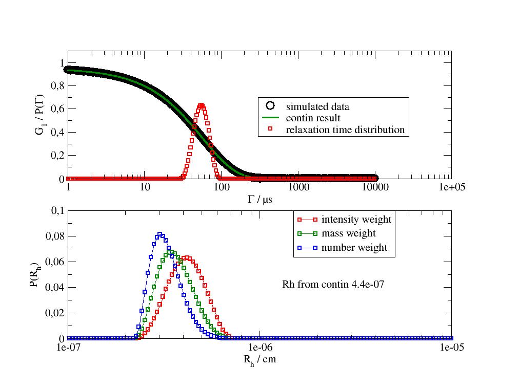
An example dataset with noise In this synthetic example the noise causes a peak width of about 20% (std/mean) as it is typically found for monodisperse samples measured short times (e.g. proteins on a Zetasizer in automatic mode). This contribution is not caused by polydispersity and always present dependent on noise level. Noise level can be reduced using longer measurement times, thus reducing the width. In real measurements one needs to test with different measurement times if polydispersity is present (thus independent on noise level).
D = 0.05 nm²/ns corresponds to a hydrodynamic radius of 4.4 nm and results in a relaxation time \(\Gamma= 1/(q^2D) \approx 58 \mu s\).
The below plots shows the CONTIN result as correlation time distribution with mean 58 µs ±12 µs and peak weight 95% in good approximation.
The second plot shows the radius distribution for different weights. Probabilities are for an interval around a point x value that the sum of all points is normalized. (not the integral on the log scale).
For real measurements one may cut noisy short times or dust contaminated long times.
import jscatter as js
import numpy as np
t=js.loglist(1,10000,1000)   #times in microseconds
q=4*np.pi*1.333/632*np.sin(np.deg2rad(90)/2) # 90 degrees for 632 nm , unit is 1/nm**2
D=0.05*1000  # nm**2/ns * 1000 = units nm**2/microseconds
noise=0.0001  # typical < 1e-3
data=js.dA(np.c_[t,0.95*np.exp(-q**2*D*t)+noise*np.random.randn(len(t))].T)

# add attributes to overwrite defaults
data.Angle      =90    # scattering angle in degrees
data.Temperature=293   # Temperature of measurement  in K
data.Viscosity  =1     # viscosity cPoise
data.Refractive =1.333 # refractive index
data.Wavelength =632   # wavelength

# do CONTIN
dr=js.dls.contin(data,distribution='x')
js.dls.contin_display(dr)         # display overview

# same to demonstrate access to distributions
bf =dr[0].contin_bestFit
p=js.grace(1.,1.)
p.multi(2,1,vgap=0.25)

# access correlation function and relaxation time distribution
p[0].plot(dr[0],sy=[1,0.5,1],legend='simulated data in [s]')
p[0].plot(dr[0].contin_result_fit,li=[1,0.2,3],sy=0,le='contin result [s]')
p[0].plot(bf._relaxationtimes,bf._intensityweightci*10,sy=[2,0.5,2],le='relaxation time distribution')
p[0].xaxis(scale='log',label=r'\xG\f{} / s',min=1e-6,max=0.1)
p[0].yaxis(label=r'G\s1\N / P(\xG\f{})',min=0,max=1.1)
p[0].legend(x=300,y=0.7)
p[0].title('Result in CONTIN units of [s]')

# Hydrodynamic radius distribution in different weights
p[1].plot(bf._hydrodynamicradii,bf._intensityweightci,sy=[2,0.5,2],li=[1,1,''],le='intensity weight')
p[1].plot(bf._hydrodynamicradii,bf._massweightci,sy=[2,0.5,3],li=[1,1,''],le='mass weight')
p[1].plot(bf._hydrodynamicradii,bf._numberweightci,sy=[2,0.5,4],li=[1,1,''],le='number weight')
p[1].xaxis(scale='log',label=r'R\sh\N / cm',min=1e-7,max=1e-5)
p[1].yaxis(label=r'P(R\sh\N)',min=0,max=0.1)
p[1].legend(x=1.5e-6,y=0.1)

# Rh of first peak
p[1].text(f'Rh from contin {bf.ipeaks[0,6]:.2g} cm',x=1.3e-6,y=0.04)
# p.save(js.examples.imagepath+'/contin.jpg')

# access peak values by
dr[0].contin_bestFit.ipeaks_name
dr[0].contin_bestFit.ipeaks
# calc std/mean of first peak
dr[0].contin_bestFit.ipeaks[0,2]/dr[0].contin_bestFit.ipeaks[0,1]
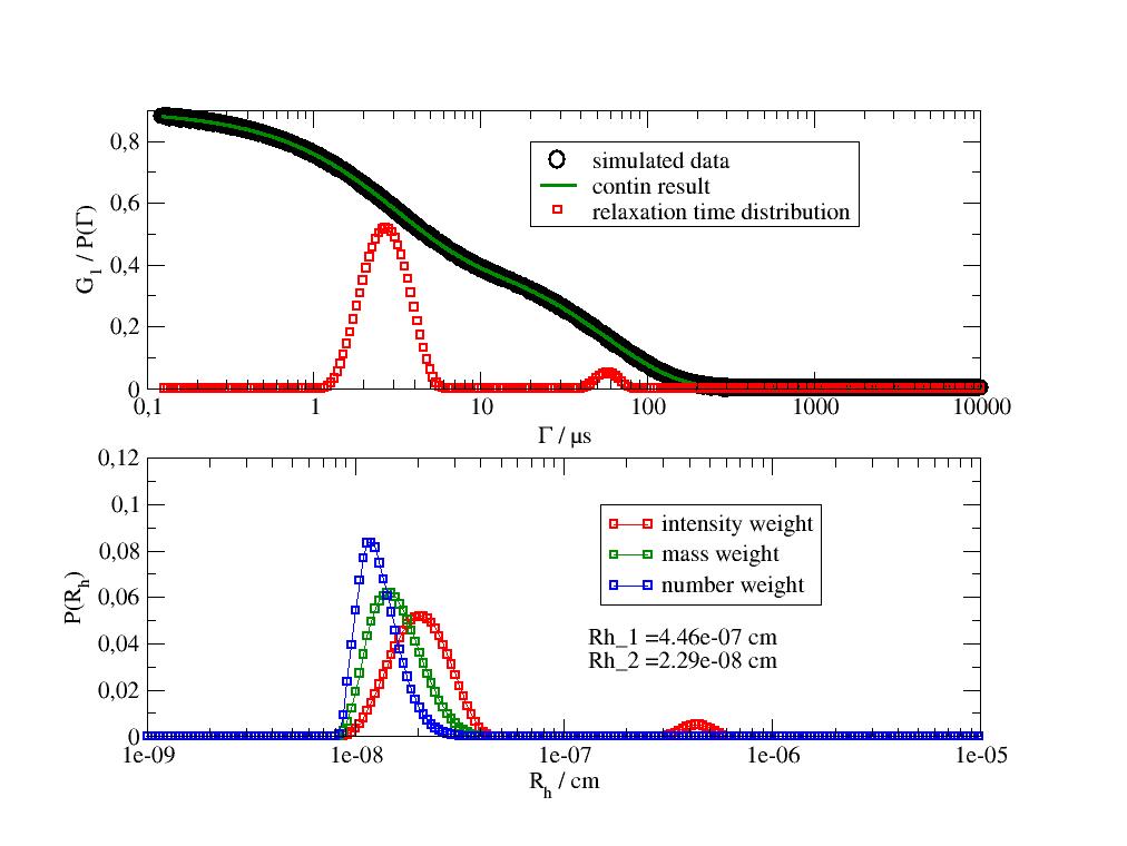
Bimodal distribution and the suppression of larger aggregates in mass and number weight. The two particles sizes with a factor of 20 in radius shows same contribution to the scattering. For mass or number weight the dependence of the scattering intensity on \(R^6\) compensates the contribution of larger aggregates.
The area under both intensity weighted peaks is equal as can be shown by integration.
import jscatter as js
import numpy as np

t=js.loglist(0.125,10000,1000)   #times in microseconds
q=4*np.pi*1.333/632*np.sin(np.deg2rad(90)/2) # 90 degrees for 632 nm , unit is 1/nm**2
D=0.05*1000  # nm**2/ns * 1000 = units nm**2/microseconds
noise=0.0001  # typical < 1e-3
data=js.dA(np.c_[t,0.45*np.exp(-q**2*D*t)+0.45*np.exp(-q**2*D*20*t) +noise*np.random.randn(len(t))].T)

# add attributes to overwrite defaults
data.Angle      =90    # scattering angle in degrees
data.Temperature=293   # Temperature of measurement  in K
data.Viscosity  =1     # viscosity cPoise
data.Refractive =1.333 # refractive index
data.Wavelength =632   # wavelength
# do CONTIN
dr=js.dls.contin(data,distribution='x')

# same to demonstrate access to distributions
bf =dr[0].contin_bestFit
p=js.grace(1.,1.)
p.multi(2,1,vgap=0.25)

# access correlation function and relaxation time distribution
p[0].plot(dr[0],sy=[1,0.5,1],legend='simulated data')
p[0].plot(dr[0].contin_result_fit,sy=[1,0.1,5],li=0,le='contin result')
p[0].plot(bf.X,bf.Y*10,sy=[2,0.5,2],le='relaxation time distribution')

p[0].xaxis(scale='log',label=r'\xG\f{} / s',min=1e-7,max=0.01)
p[0].yaxis(label=r'G\s1\N / P(\xG\f{})')
p[0].legend(x=20e-6,y=0.8)

# Hydrodynamic radius distribution in different weights
p[1].plot(bf._hydrodynamicradii,bf._intensityweightci, sy=[2,0.5,2],li=[1,1,''],le='intensity weight')
p[1].plot(bf._hydrodynamicradii,bf._massweightci, sy=[2,0.5,3],li=[1,1,''],le='mass weight')
p[1].plot(bf._hydrodynamicradii,bf._numberweightci, sy=[2,0.5,4],li=[1,1,''],le='number weight')
p[1].xaxis(scale='log',label=r'R\sh\N / cm',min=1e-9,max=1e-5)
p[1].yaxis(label=r'P(R\sh\N)',min=0,max=0.12)
p[1].legend(x=1.5e-7,y=0.1)

# Rh of first two peaks
p[1].text(fr'Rh_1 ={bf.ipeaks[0,6]:.3g} cm \nRh_2 ={bf.ipeaks[1,6]:.3g} cm',x=1.3e-7,y=0.04)
# p.save(js.examples.imagepath+'/contin_bimodal.jpg')

# Peak integration resulting in about 0.5 for both
p1=(1<bf.X) &(bf.X<20) # peak borders 10 and 100
fp1 = np.trapezoid(bf.Y[p1],bf.X[p1])/np.trapezoid(bf.Y,bf.X) #
p2 = (40<bf.X) &(bf.X<400) # peak borders 10 and 100
fp2 = np.trapezoid(bf.Y[p2],bf.X[p2])/np.trapezoid(bf.Y,bf.X) #
# p.save(js.examples.imagepath+'/contin_bimodal.jpg')
R20 (scattering vector) is calculated as R20= 4e-7*pi*R15/R16*sin(R17/2), if R16!=0. else R20=0
References
[1]CONTIN: A general purpose constrained regularization program for inverting noisy linear algebraic and integral equations Provencher, S Computer Physics Communications 27: 229.(1982) doi:10.1016/0010-4655(82)90174-6.
[3]A constrained regularization method for inverting data represented by linear algebraic or integral equations Provencher, S. W. Comp. Phys. Commu 27: 213–227. (1982) doi:10.1016/0010-4655(82)90173-4
[4]Inverse problems in polymer characterization: Direct analysis of polydispersity with photon correlation spectroscopy. S.W. Provencher, Makromol. Chem. 180, 201 (1979).
[5]Transformation Properties of Probability Density Functions Stanislav Sýkora Permalink via DOI: 10.3247/SL1Math04.001
Original code description in CONTIN
C  THE FOLLOWING ARE THE NECESSARY INPUT -                                  0460
C                                                                           0461
C  DOUSIN = T (DOUSIN MUST ALWAYS BE .TRUE..)                               0462
C                                                                           0463
C  LUSER(3) = T, TO HAVE FORMF2, THE SQUARED FORM FACTORS, COMPUTED IN      0464
C                USERK.                                                     0465
C           = F, TO SET ALL THE FORMF2 TO 1. (AS WOULD BE APPROPRIATE       0466
C                WITH LAPLACE TRANSFORMS).                                  0467
C  RUSER(24) MAY BE NECESSARY INPUT TO SPECIFY THE FORM FACTOR (E.G.,       0468
C            THE WALL THICKNESS OF A HOLLOW SPHERE) IF LUSER(3)=T.  SEE     0469
C            COMMENTS IN USERK.                                             0470
C  IUSER(18) MAY BE NECESSARY INPUT IF LUSER(3)=T (E.G., TO SPECIFY THE     0471
C            NUMBER OF POINTS OVER WHICH THE SQUARED FORM FACTORS WILL      0472
C            BE AVERAGED). SEE COMMENTS IN USERK.                           0473
C                                                                           0474
C  RUSER(16) = WAVELENGTH OF INCIDENT LIGHT (IN NANOMETERS),                0475
C            = 0, IF RUSER(20), THE MAGNITUDE OF THE SCATTERING VECTOR      0476
C                 (IN CM**-1), IS NOT TO BE COMPUTED.  WHEN                 0477
C                 RUSER(16)=0, RUSER(15) AND RUSER(17) NEED NOT BE          0478
C                 INPUT, AND CONTIN WILL SET RUSER(21)=1                    0479
C                 (AS APPROPRIATE WITH LAPLACE TRANSFORMS).                 0480
C                                                                           0481
C  RUSER(15) = REFRACTIVE INDEX.                                            0482
C  RUSER(17) = SCATTERING ANGLE (IN DEGREES).                               0483
C                                                                           0484
C                                                                           0485
C  IUSER(10) SELECTS SPECIAL CASES OF USERK FOR MORE CONVENIENT USE.        0486
C                                                                           0487
C  IUSER(10) = 1, FOR MOLECULAR WEIGHT DISTRIBUTIONS FROM PCS               0488
C                 (WHERE THE SOLUTION, S(G), IS SUCH THAT S(G)DG IS         0489
C                 THE WEIGHT FRACTION WITH MOLECULAR WEIGHT BETWEEN         0490
C                 G AND G+DG).                                              0491
C                 CONTIN SETS -                                             0492
C                   RUSER(23) = 1.,                                         0493
C                   RUSER(21) = RUSER(18)*RUSER(20)**2.                     0494
C                               (SEE ABOVE DISCUSSION OF RUSER(16).)        0495
C                 YOU MUST INPUT -                                          0496
C                   RUSER(18) TO SATISFY THE EQUATION (IN CGS UNITS) -      0497
C                   (DIFFUSION COEFF.)=RUSER(18)*(MOL. WT.)**RUSER(22).     0498
C                   RUSER(22) (MUST ALSO BE INPUT, TYPICALLY ABOUT -.5).    0499
C                                                                           0500
C  IUSER(10) = 2, FOR DIFFUSION-COEFFICIENT DISTRIBUTONS OR LAPLACE         0501
C                 TRANSFORMS (WHERE G IS DIFF. COEFF. IN CM**2/SEC          0502
C                 OR, E.G., TIME CONSTANT).                                 0503
C                 CONTIN SETS -                                             0504
C                   RUSER(23) = 0.,                                         0505
C                   RUSER(22) = 1.,                                         0506
C                   RUSER(21) = RUSER(20)**2 (SEE ABOVE DISCUSSION          0507
C                                             OF RUSER(16).).               0508
C                                                                           0509
C  IUSER(10) = 3, FOR SPHERICAL-RADIUS DISTRIBUTIONS, ASSUMING THE          0510
C                 EINSTEIN-STOKES RELATION (WHERE THE SOLUTION, S(G),       0511
C                 IS SUCH THAT S(G)DG IS THE WEIGHT FRACTION OF             0512
C                 PARTICLES WITH RADIUS (IN CM) BETWEEN G AND G+DG.         0513
C                 WEIGHT-FRACTION DISTRIBUTIONS YIELD BETTER SCALED         0514
C                 PROBLEMS THAN NUMBER-FRACTION DISTRIBUTIONS, WHICH        0515
C                 WOULD REQUIRE RUSER(23)=6.)                               0516
C                 CONTIN SETS -                                             0517
C                   RUSER(23) = 3.,                                         0518
C                   RUSER(22) = -1.,                                        0519
C                   RUSER(21) = RUSER(20)**2*(BOLTZMANN CONST.)*            0520
C                               RUSER(18)/(.06*PI*RUSER(19)).               0521
C                               (SEE ABOVE DISCUSSION OF RUSER(16).)        0522
C                 YOU MUST HAVE INPUT -                                     0523
C                   RUSER(18) = TEMPERATURE (IN DEGREES KELVIN),            0524
C                   RUSER(19) = VISCOSITY (IN CENTIPOISE).                  0525
C                                                                           0526
C  IUSER(10) = 4, FOR GENERAL CASE, WHERE YOU MUST HAVE INPUT -             0527
C                 RUSER(J), J = 21, 22, 23.                                 0528
C                                                                           0529
C                                                                           0530
- jscatter.dls.contin_display(result_list, select=None, npeak=2, *args, **kw)[source]
A routine to plot CONTIN results to get an overview over CONTIN output.
- Parameters:
- result_listdataList
Output of dls.contin.
- selectlist of int
Sequence of integers in result_list to select for output.
- npeakint
Number of peaks in output default 2.
- dlogy
shows distribution in y logscale
Notes
access diffusion of all first peaks by output[:,1,6]mean and std asoutput[:,1,6].mean()output[:,1,6].std()
- jscatter.dls.readZetasizerNano(filename, NANOcoding='cp1257', NANOlocale=None)[source]
Read ASCII file data exported from Malvern Zetasizer Nano (.csv format).
Format of Zetasizer is ‘.csv’ with one measurement per line as defined in the export macro. First line gives names of columns as header line, so header line in NANO export is necessary. Lists as Sizes, Volumes… need to be separated by “sample name” because of different length. Only ‘Size’ lines are read as datalines.
- Parameters:
- filenamestring
Zetasizer filename
- NANOcodingstring
UTF coding from Windows
- NANOlocalelist of string
- encoding of weekday names in NAno textfile[‘de_DE’,’UTF-8’] NANO set to German[‘en_US’,’UTF-8’] NANO set to US…
- Returns:
- dataList with dataArray for each measurement
Dataarray contains :
correlation data [CorrelationDelayTime; g1; g2minus1] (if present otherwise empty dataArray)
.distributions : Distribution fits with columns
[RelaxationTimes, Sizes, Intensities, Volumes, Diffusions] (if present)
fit results of correlation function in attributes (some channels are discarded -> see Zetasizer settings)
.distributionFitDelayTimes timechannels
.distributionFitData measured points
.distributionFit fit result
Check .attr for more attributes like SampleName, MeanCountRate, SizePeak1mean, SizePeak1width, Temperature
If no correlation or distributions are present the data are zero and only parameters are stored. No unit conversion is done.
Notes
Zetasizer software saves \(g_2-1=g_1^2\) which can also be used for fitting and may be prefered for fitting.
CorrelationData.Y contains \(g_1 = sign(g_2-1)|g_2-1|^{1/2}))\) to preserve noise distribution around 0 and not to bias \(g_1\) to positive values.
Zeros in data are from original read data file related to the instrument software.
The template for export in Zetasizer has some requirements:
The header line should be included.
Separator is the tab.
First entries should be “Serial Number” “Type” “Sample Name” “Measurement Date and Time”
Sequence data as “Sizes”, “Intensities” should be separated by “Sample Name” as separator.
Appending to same file is allowed if new header line is included.
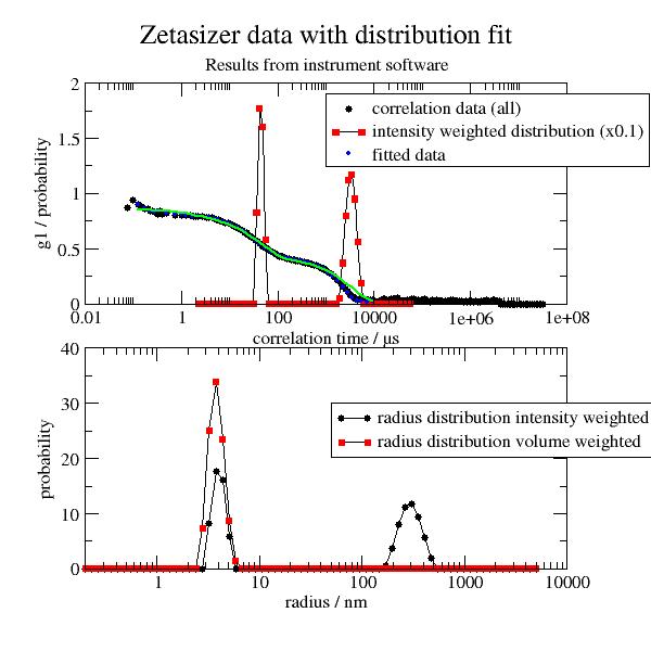
Examples
import jscatter as js
import numpy as np
# read example data
alldls = js.dls.readZetasizerNano(js.examples.datapath + '/dlsPolymerSolution.txt', NANOlocale=['de_DE', 'UTF-8'])
one=alldls[5]
p=js.grace()
p.multi(2,1,vgap=0.2)
p[0].plot(one,legend='correlation data (all)')
p[0].plot(one.distributions.X, one.distributions.Y /  10 , li=1, legend='intensity weighted distribution (x0.1)')
p[0].plot(one.DistributionFitDelayTimes,one.DistributionFitData,sy=[1,0.2,4],le='fitted data')
p[0].plot(one.DistributionFitDelayTimes,one.DistributionFit,sy=0,li=[1,2,5])
p[1].plot(one.distributions[1], one.distributions[2] , li=1, legend='radius distribution intensity weighted')
p[1].plot(one.distributions._Sizes, one.distributions._Volumes, li=1, legend='radius distribution volume weighted')

p[0].xaxis(scale='l', label=r'correlation time / µs ', tick=[10, 9])
p[1].xaxis(scale='l', label=r'radius / nm ')
p[0].yaxis(label=r'g1 / probability ')
p[1].yaxis(label=r'probability ')
p[0].legend(x=1000,y=1.9)
p[1].legend(x=50,y=30)
p[0].title('Zetasizer data with distribution fit')
p[0].subtitle('Results from instrument software')
# p.save(js.examples.imagepath+'/Zetasizerexample.jpg',format='jpeg',size=[600/300,600/300]) #as jpg file