5. smallanglescattering (sas)

This module allows smearing/desmearing of SAXS/SANS data and provides the sasImage class to read and analyse 2D detector images from SAXS cameras.

• Smearing is for line collimation as in Kratky SAXS cameras and for point collimation as SAXS/SANS data. For point collimation the resolution smearing a la Pedersen is realised. This can also be used for SAXS instruments in pinhole geometry collimation with smaller pinholes and distances. Smearing as decorator of model allows simultaneous fit of smeared data from SANS/SAXS at different collimations.

• Desmearing uses the Lake algorithm as an iterative procedure to desmear measured data. We follow here the improvements according to Vad using a convergence criterion and smoothing.

• 2D SAXS data can be read into sasImage to do typical tasks as transmission correction, masking, beamcenter location, 2D background subtraction, radial average (also for sectors).

• Transmission correction and background correction are explained in Analyse SAS data

• As references the waterXray scattering and a AgBe reference spectrum are available.

• For form factors and structure factors see the respective modules. Conversion of sasImage to dataArray allows 2D fit of scattering patterns (see Fitting the 2D scattering of a lattice)

5.1. SAS smear/desmear 1D

The preferred method for convolution with instrument resolution is smear. smear modifies model functions to automatically extend the q range beyond edges for proper smearing as needed to fit smeared SANS/SAXS data. Smearing explicit data by smear or resFunct needs additional information how to extrapolate data at the detector edges. See smear for detailed explanation. Needed beamProfiles are prepared by prepareBeamProfile.

smear([unsmeared, beamProfile])	Smearing model/data for point collimation SANS/SAXS or line-collimated SAXS (Kratky camera) allowing simultaneous SAXS/SANS fitting.
desmear(Ios, beamProfile[, NIterations, ...])	Desmearing of measured data according to Lake algorithm with possibility to stop recursion at best desmearing.
resFunct(S[, collDist, collAperture, ...])	Resolution smearing of small angle scattering for SANS/SAXS according to Pedersen for radial averaged data.
resFunctExplicit(S, beamprofile[, extrapolfunc])	Resolution smearing of small angle scattering for SANS/SAXS according to explict given Gaussian width in unit 1/nm.
prepareBeamProfile([data])	Prepare beamProfile from beam profile measurement or according to given parameters.
getBeamWidth(empty[, minmax, show])	Extract primary beam of empty cell or buffer measurement for semitransparent beam stops.
plotBeamProfile(beam[, p])	Plots beam profile and weight function according to parameters in beam.

5.2. SAS convenience

transmissionCorrection(data[, dark, ...])	Subtract dark current, find primary beam, get transmission count and normalize by transmission and exposure time.
waterXrayScattering([composition, T, units])	Absolute scattering of water with components (salt, buffer) at Q=0 as reference for X-ray.
AgBeReference(q, wavelength[, n, ampn, ...])	The scattering intensity expected from AgBe as a reference for wavelength calibration.

5.3. 2D sasImage

Read 2D image files from SAXS cameras and extract the corresponding data.

The sasImage is a 2D array that allows direct subtraction and multiplication (e.g. transmission) respecting given masks in operations. E.g.

sample=js.sas.sasImage('sample.tiff')
solvent=js.sas.sasImage('solvent.tiff')
corrected = sample/sampletransmission - solvent/solventtransmission

• Image manipulation like Gaussian filter from scipy.ndimage can be used.

• Calibration of detector distance including offset detector positions, radial average, size reduction and more. .pickCenter allows sensitive detection of the beamcenter in SAS geometry. .calibrateOffsetDetector allows sensitive calibration of the detector position parameters.

• TIFF images are read directly. Other image formats as .edf can be treated using the library fabio. Example is given in sasImage .

Examples are shown in sasImage including reading of different images produced by 2D X-ray detectors using the fabio library.

---

sasImage(file[, detector_distance, center, ...])

Creates/reads sasImage as maskedArray from a detector image or array.

5.3.1. sasImage methods

Create above sasImage im = sasImage('image.tif') and use following methods like im.array.

Proccessing/Calibration

asImage([scale, colormap, inverse, ...])	Returns the sasImage as 8bit RGB image using PIL.
saveAsTIF(filename[, fill])	Save the sasImage as float32 tif without loosing information.
radialAverage([center, number, kind, ...])	Radial average of image and conversion to wavevector q.
azimuthAverage([center, qrange, number, ...])	Azimuthal average of image and conversion to wavevector q.
recalibrateDetDistance([center, number, ...])	Recalibration of detectorDistance by AgBe reference for point collimation.
calibrateOffsetDetector([lattice, center, ...])	Compare sasImage to calibration standard in powder average to determine detector position.
gaussianFilter([sigma])	Gaussian filter in place.
getPolar([center, scaleR, offset])	Transform to polar coordinates around center with interpolation.
showPolar([center, scaleR, offset, scale])	Show image transformed to polar coordinates around center.
reduceSize([bin, center, border])	Reduce size of image using uniform average in box.
show(**kwargs)	Show sasImage as matplotlib figure.
array	Strip of all attributes and return a simple array without mask.
asdataArray([masked])	Return representation of sasImage as dataArray with (qx, qy, qz, I(qx,qy,qz)).
interpolateMaskedRadial([radial])	Interpolate masked values from radial averaged image or function.
pickBeamcenter([levels, symmetry])	Pick the beam center from a calibration sample as AgBe in standard SAS geometry if a beamstop is used.
findCenterOfIntensity([center, size])	Find beam center as center of intensity..

line collimation feature

lineFindCenter([minmax, use, show, darkline])	Find center of primary beam for line collimation cameras with semitransparent beamstop.
lineAverage([sigma, darkline, whiteline])	Line average and conversion to wavevector q for Kratky (line) collimation cameras.

Masking

maskReset()	Reset the mask.
maskFromImage(image)	Use/copy mask from image.
maskRegion(xmin, xmax, ymin, ymax)	Mask rectangular region.
maskRegions(regions)	Mask several regions.
maskbelowLine(p1, p2)	Mask points at one side of line.
maskTriangle(p1, p2, p3[, invert])	Mask inside triangle.
mask4Polygon(p1, p2, p3, p4[, invert])	Mask inside polygon of 4 points.
maskCircle(center, radius[, invert])	Mask points inside circle.
maskSectors(angles, width[, radialmax, invert])	Mask sector around center.

Attributes

pQ	3D scattering vector \(q\) for pixels with detector placed in standard SAS or offset geometry.
pQnorm	3D scattering vector \(|q|\) for detector pixel.
pQaxes()	Get scattering vector along detector pixel axes X, Y around center.
attr	Show specific attribute names as sorted list of attribute names.
showattr([maxlength, exclude])	Show specific attributes with values as overview.
setAttrFromImage(image)	Copy center, detector_distance, alpha, beta, gamma wavelength, pixel_size from image.
setDetectorPosition(center, detector_distance)	Set parameters describing the position and orientation of the detector.
setDetectorDistance(detector_distance)	Set detector distance as shortest distance to sample along plane normal vector.
setPlaneCenter(center)	Set beamcenter or center of detector plane where plane normal has shortest distance to sample.
setPlaneOrientation([alpha, beta, gamma])	Set orientation angles of detector plane .
setPixelSize(pixel_size)	Set pixel_size.
setWavelength(wavelength)	Set wavelength.
getfromcomment(name[, replace, newname])	Extract name from .artist or .imageDescription with attribute name in front.

5.4. 2D sasImage convenience

createLogPNG(filenames[, center, size, ...])	Create .png files from grayscale images with log scale conversion to values between [1,255].
createImageDescriptions(images)	Create text file with image descriptions as list of content.
readImages(filenames[, onlyheaders])	Read a list of images returning sasImage`s.

5.5. Housekeeping

readpdh(pdhFileName)	Opens and reads a SAXS data file in the .pdh (Primary Data Handling) format.
autoscaleYinoverlapX(dataa[, key, keep])	Scales elements of data to have same mean .Y value in the overlap region of .X .
removeSpikesMinmaxMethod(dataa[, order, ...])	Takes a dataset and removes single spikes from data by substitution with spline.
removeSpikes(dataa[, xmin, xmax, medwindow, ...])	Takes a dataset and removes single spikes.
locateFiles(pattern[, root])	Locate all files matching supplied filename pattern in and below supplied root directory.
copyFiles(pattern[, root, destination, link])	Copies all files matching pattern in tree below root to destination directory
addXMLParameter(data)	Adds the parameters stored in xml part of a .pdh file as eg.
moveSAXSPACE(pattern[, root, destination, ...])	Read SAXSPACE .pdh files and removes spikes by removeSpikes.

---

This module allows smearing/desmearing of SAXS/SANS data and provides the sasImage class to read and analyse 2D detector images from SAXS cameras.

• Smearing is for line collimation as in Kratky SAXS cameras and for point collimation as SAXS/SANS data. For point collimation the resolution smearing a la Pedersen is realised. This can also be used for SAXS instruments in pinhole geometry collimation with smaller pinholes and distances. Smearing as decorator of model allows simultaneous fit of smeared data from SANS/SAXS at different collimations.

• Desmearing uses the Lake algorithm as an iterative procedure to desmear measured data. We follow here the improvements according to Vad using a convergence criterion and smoothing.

• 2D SAXS data can be read into sasImage to do typical tasks as transmission correction, masking, beamcenter location, 2D background subtraction, radial average (also for sectors).

• Transmission correction and background correction are explained in Analyse SAS data

• As references the waterXray scattering and a AgBe reference spectrum are available.

• For form factors and structure factors see the respective modules. Conversion of sasImage to dataArray allows 2D fit of scattering patterns (see Fitting the 2D scattering of a lattice)

jscatter.sas.AgBeReference(q, wavelength, n=array([1, 2, 3, 4, 5, 6, 7, 8, 9]), ampn=None, domainsize=100, udw=0.1, asym=0, lg=1)

The scattering intensity expected from AgBe as a reference for wavelength calibration.

The intensities assume a d-spacing of 5.8378 nm and a reduction of the intensity as q**-2. The domain size determines the width according to Scherrer equation [2]. The first peak is at 1.076 1/nm. The result needs to be convoluted with the instrument resolution by resFunct or smear. Here only the main planes of AgBe are taken into account. See example.

Parameters:

qarray

Wavevector in units 1/nm.

wavelengthfloat

Wavelength, units nm.

narray of int

Order of the peaks to calculate.

ampnlist of float

Amplitudes of the peaks.

domainsizefloat

Domainsize of AgBe crystals in nm. default 100 nm as is given in [1].

udwfloat

Displacement u in Debye Waller factor exp(-u**2*q**2/3) in units nm.

asymfloat

Factor asymmetry in Voigt function describing the peaks.

lgfloat

Lorenzian/gaussian fraction of both FWHM, describes the contributions of gaussian and lorenzian shape. See Voigt for details.

Returns:

dataArray

References

[1]

T. C. Huang, H. Toraya, T. N. Blanton and Y. Wu X-ray Powder Diffraction Analysis of Silver Behenate, a Possible Low-Angle Diffraction Standard J. Appl.Cryst.(1993).26,180-184

[2]

Patterson, A. The Scherrer Formula for X-Ray Particle Size Determination Phys. Rev. 56 (10): 978–982 (1939) doi:10.1103/PhysRev.56.978.

Examples

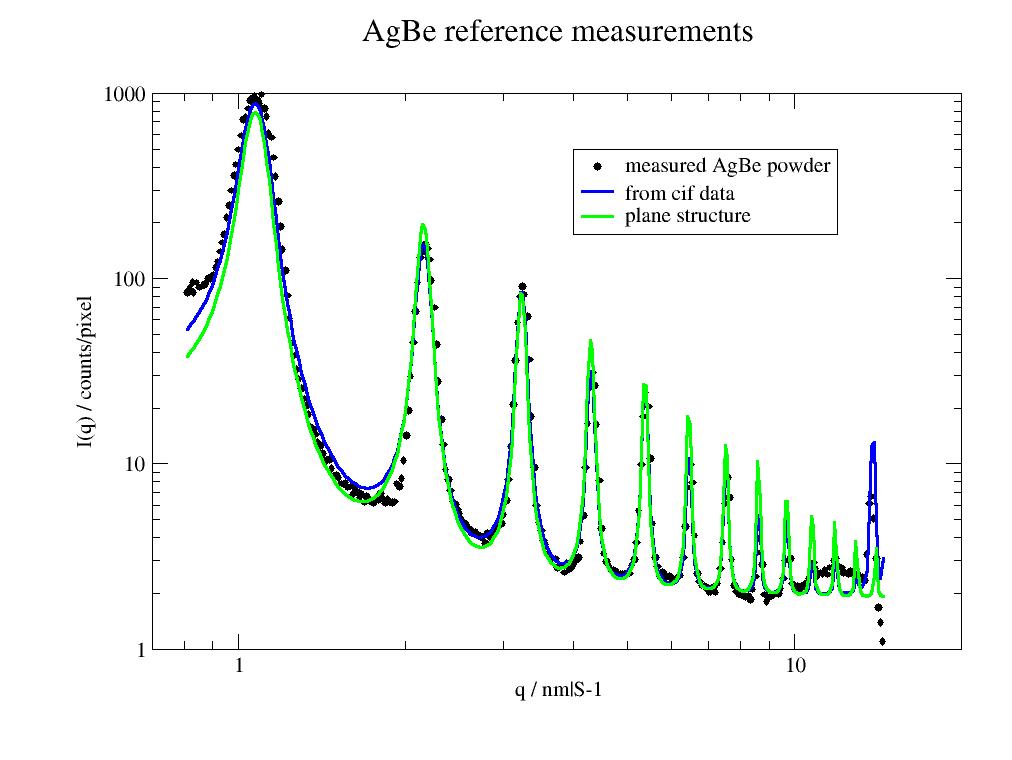
Xray AgBe measurement

The simplified plane model is good enough for peak determination while the crystallographic model gets the high order peaks intensities better.

import numpy as np
import jscatter as js

#
# Look at raw calibration measurement
calibration = js.sas.sasImage(js.examples.datapath+'/calibration.tiff')
bc=calibration.center
calibration.mask4Polygon([bc[0]+8,bc[1]],[bc[0]-8,bc[1]],[bc[0]-8+60,0],[bc[0]+8+60,0])
# mask center
calibration.maskCircle(calibration.center, 18)
# mask outside shadow
calibration.maskCircle([500,320], 280,invert=True)
# calibration.show(axis='pixel',scale='log')
cal=calibration.radialAverage()

# lattice from crystallographic data in cif file.
agbe=js.sf.latticeFromCIF(js.examples.datapath + '/1507774.cif',size=[0,0,0])
sfagbe=js.sf.latticeStructureFactor(cal.X, lattice=agbe,
                                   domainsize=50, rmsd=0.001, lg=1, hklmax=17,wavelength=0.15406)

# simplified model of planes
ag = js.sas.AgBeReference(q=sfagbe.X, wavelength=0.13414, n=np.r_[1:14], domainsize=50)

p=js.grace()
p.plot(cal, le='measured AgBe powder')
# add scaling and background (because of unscaled raw data)
p.plot(sfagbe.X,190*sfagbe.Y+1.9,sy=0,li=[1,3,4],legend='from cif data')
p.plot(ag.X, ag.Y*3+1.9, sy=0, li=[1,3,5],le='plane structure')
p.yaxis(scale='log',label='I(q) / counts/pixel')
p.xaxis(scale='log',label='q / nm|S-1',min=0.7,max=20)
p.title('AgBe reference measurements')
p.legend(x=4,y=500)
# p.save(js.examples.imagepath+'/AgBeplanes.jpg')

SANS calibration check To verify a calibration measurement using a AgBe we use our AgBeReference and allow for a change of Q and wavelength in the model to get a new wavelength. This assumes that the used wavelength for Q determination was wrong. Here we include a resolution from SANS and use wavespread as additional fir parameter.

This function can be used to fit the SANS measurement.

resolution = js.sas.prepareBeamProfile('SANS', detDist=1100,collDist=4000.,wavelength=0.3,wavespread=0.15,
                                   collAperture=30, sampleAperture=8, dpixelWidth=10, dringwidth=1)

@js.sas.smear(beamProfile=resolution)
def ref(q,newwave,wavespread,amp,detDist,collDist,bgr0,dsize,udw,asym,lg,ampn0,ampn1,ampn2):
    # old wavelength
    oldwave = 0.3 # unit nm
    # rescale q and calc reference including the first 3 peaks
    I=js.sas.AgBeReference(q*oldwave/newwave,newwave,udw=udw,domainsize=dsize,lg=lg,
                                               asym=asym,ampn=[ampn0,ampn1,ampn2])
    I.X = q  # restore old q
    I.Y=I.Y * amp + bgr0  # scale intensity and add background
    return I

class jscatter.sas.Button(ax, label, image=None, color='0.85', hovercolor='0.95', *, useblit=True)

Bases: AxesWidget

Parameters:

ax~matplotlib.axes.Axes

The ~.axes.Axes instance the button will be placed into.

labelstr

The button text.

imagearray-like or PIL Image

The image to place in the button, if not None. The parameter is directly forwarded to ~.axes.Axes.imshow.

color:mpltype:`color`

The color of the button when not activated.

hovercolor:mpltype:`color`

The color of the button when the mouse is over it.

useblitbool, default: True

Use blitting for faster drawing if supported by the backend. See the tutorial blitting for details.

Added in version 3.7.

disconnect(cid)

Remove the callback function with connection id cid.

on_clicked(func)

Connect the callback function func to button click events.

Returns a connection id, which can be used to disconnect the callback.

class jscatter.sas.Circle(xy, radius=5, **kwargs)

Bases: Ellipse

Create a true circle at center xy = (x, y) with given radius.

Unlike CirclePolygon which is a polygonal approximation, this uses Bezier splines and is much closer to a scale-free circle.

Valid keyword arguments are:

Properties:

agg_filter: a filter function, which takes a (m, n, 3) float array and a dpi value, and returns a (m, n, 3) array and two offsets from the bottom left corner of the image alpha: unknown animated: bool antialiased or aa: bool or None capstyle: .CapStyle or {‘butt’, ‘projecting’, ‘round’} clip_box: ~matplotlib.transforms.BboxBase or None clip_on: bool clip_path: Patch or (Path, Transform) or None color: :mpltype:`color` edgecolor or ec: :mpltype:`color` or None edgegapcolor: :mpltype:`color` or None facecolor or fc: :mpltype:`color` or None figure: ~matplotlib.figure.Figure or ~matplotlib.figure.SubFigure fill: bool gid: str hatch: {‘/’, ‘\’, ‘|’, ‘-’, ‘+’, ‘x’, ‘o’, ‘O’, ‘.’, ‘*’} hatch_linewidth: unknown hatchcolor: :mpltype:`color` or ‘edge’ or None in_layout: bool joinstyle: .JoinStyle or {‘miter’, ‘round’, ‘bevel’} label: object linestyle or ls: {‘-’, ‘–’, ‘-.’, ‘:’, ‘’, …} or (offset, on-off-seq) linewidth or lw: float or None mouseover: bool path_effects: list of .AbstractPathEffect picker: None or bool or float or callable rasterized: bool sketch_params: (scale: float, length: float, randomness: float) snap: bool or None transform: ~matplotlib.transforms.Transform url: str visible: bool zorder: float

get_radius()

Return the radius of the circle.

property radius

Return the radius of the circle.

set(*, agg_filter=<UNSET>, alpha=<UNSET>, angle=<UNSET>, animated=<UNSET>, antialiased=<UNSET>, capstyle=<UNSET>, center=<UNSET>, clip_box=<UNSET>, clip_on=<UNSET>, clip_path=<UNSET>, color=<UNSET>, edgecolor=<UNSET>, edgegapcolor=<UNSET>, facecolor=<UNSET>, fill=<UNSET>, gid=<UNSET>, hatch=<UNSET>, hatch_linewidth=<UNSET>, hatchcolor=<UNSET>, height=<UNSET>, in_layout=<UNSET>, joinstyle=<UNSET>, label=<UNSET>, linestyle=<UNSET>, linewidth=<UNSET>, mouseover=<UNSET>, path_effects=<UNSET>, picker=<UNSET>, radius=<UNSET>, rasterized=<UNSET>, sketch_params=<UNSET>, snap=<UNSET>, transform=<UNSET>, url=<UNSET>, visible=<UNSET>, width=<UNSET>, zorder=<UNSET>)

Set multiple properties at once.

a.set(a=A, b=B, c=C)

is equivalent to

a.set_a(A)
a.set_b(B)
a.set_c(C)

In addition to the full property names, aliases are also supported, e.g. set(lw=2) is equivalent to set(linewidth=2), but it is an error to pass both simultaneously.

The order of the individual setter calls matches the order of parameters in set(). However, most properties do not depend on each other so that order is rarely relevant.

Supported properties are

Properties:

agg_filter: a filter function, which takes a (m, n, 3) float array and a dpi value, and returns a (m, n, 3) array and two offsets from the bottom left corner of the image alpha: float or None angle: float animated: bool antialiased or aa: bool or None capstyle: .CapStyle or {‘butt’, ‘projecting’, ‘round’} center: (float, float) clip_box: ~matplotlib.transforms.BboxBase or None clip_on: bool clip_path: Patch or (Path, Transform) or None color: :mpltype:`color` edgecolor or ec: :mpltype:`color` or None edgegapcolor: :mpltype:`color` or None facecolor or fc: :mpltype:`color` or None figure: ~matplotlib.figure.Figure or ~matplotlib.figure.SubFigure fill: bool gid: str hatch: {‘/’, ‘\’, ‘|’, ‘-’, ‘+’, ‘x’, ‘o’, ‘O’, ‘.’, ‘*’} hatch_linewidth: unknown hatchcolor: :mpltype:`color` or ‘edge’ or None height: float in_layout: bool joinstyle: .JoinStyle or {‘miter’, ‘round’, ‘bevel’} label: object linestyle or ls: {‘-’, ‘–’, ‘-.’, ‘:’, ‘’, …} or (offset, on-off-seq) linewidth or lw: float or None mouseover: bool path_effects: list of .AbstractPathEffect picker: None or bool or float or callable radius: float rasterized: bool sketch_params: (scale: float, length: float, randomness: float) snap: bool or None transform: ~matplotlib.transforms.Transform url: str visible: bool width: float zorder: float

set_radius(radius)

Set the radius of the circle.

Parameters:

radiusfloat

class jscatter.sas.LinearNDInterpolator(points, values, fill_value=np.nan, rescale=False)

Bases: NDInterpolatorBase

Check shape of points and values arrays, and reshape values to (npoints, nvalues). Ensure the points and values arrays are C-contiguous, and of correct type.

class jscatter.sas.NearestNDInterpolator(x, y, rescale=False, tree_options=None)

Bases: NDInterpolatorBase

Check shape of points and values arrays, and reshape values to (npoints, nvalues). Ensure the points and values arrays are C-contiguous, and of correct type.

class jscatter.sas.PickerBeamCenter(circle, image, destination, symmetry=6)

Bases: object

Class to pick the center of calibration sasImage

circle :

Circle around center to move

image :

image to use for calculation of profiles

destination :

axes where to plot profiles

symmetry :

number of sectors to use for averaging

on_button_press(event)

on_keypress(event)

on_scroll(event)

update()

class jscatter.sas.PickerDetPosition(image, lattice, axes, buttons, latticeparameters)

Bases: object

Class to pick the detector position of calibration sasImage

We have 2 axes with the image and the lines to align. We use buttons to update the image parameters directly and use a single update method for all.

balpha_m(event)

balpha_p(event)

bastep(event)

bbeta_m(event)

bbeta_p(event)

bcenterx_m(event)

bcenterx_p(event)

bcentery_m(event)

bcentery_p(event)

bcstep(event)

bdistance_m(event)

bdistance_p(event)

bgamma_m(event)

bgamma_p(event)

bstep(event)

on_button_press(event)

update()

class jscatter.sas.Rotation(quat: ArrayLike, normalize: bool = True, copy: bool = True, scalar_first: bool = False)

Bases: object

Rotation in 3 dimensions.

This class provides an interface to initialize from and represent rotations with:

• Quaternions

• Rotation Matrices

• Rotation Vectors

• Modified Rodrigues Parameters

• Euler Angles

• Davenport Angles (Generalized Euler Angles)

The following operations on rotations are supported:

• Application on vectors

• Rotation Composition

• Rotation Inversion

• Rotation Indexing

A Rotation instance can contain a single rotation transform or rotations of multiple leading dimensions. E.g., it is possible to have an N-dimensional array of (N, M, K) rotations. When applied to other rotations or vectors, standard broadcasting rules apply.

Indexing within a rotation is supported to access a subset of the rotations stored in a Rotation instance.

To create Rotation objects use from_... methods (see examples below). Rotation(...) is not supposed to be instantiated directly.

Parameters:

quatarray_like, shape (…, 4)

Quaternion representing the rotation.

normalizebool, optional

If True, orthonormalize the rotation matrix using singular value decomposition. If False, the rotation matrix is not checked for orthogonality or right-handedness.

copybool, optional

If True, copy the input matrix. If False, a reference to the input matrix is used. If normalize is True, the input matrix is always copied regardless of the value of copy.

scalar_firstbool, optional

If True then quat is expect in scalar-first format otherwise it is expected in scalar-last format. Defaults to False.

Attributes:

single

Whether this instance represents a single rotation.

Methods

__len__()	Number of rotations contained in this object.
from_quat(quat, *[, scalar_first])	Initialize from quaternions.
from_matrix(matrix, *[, assume_valid])	Initialize from rotation matrix.
from_rotvec(rotvec[, degrees])	Initialize from rotation vectors.
from_mrp(mrp)	Initialize from Modified Rodrigues Parameters (MRPs).
from_euler(seq, angles[, degrees])	Initialize from Euler angles.
from_davenport(axes, order, angles[, degrees])	Initialize from Davenport angles.
as_quat([canonical, scalar_first])	Represent as quaternions.
as_matrix()	Represent as rotation matrix.
as_rotvec([degrees])	Represent as rotation vectors.
as_mrp()	Represent as Modified Rodrigues Parameters (MRPs).
as_euler(seq[, degrees, suppress_warnings])	Represent as Euler angles.
as_davenport(axes, order[, degrees, ...])	Represent as Davenport angles.
concatenate(rotations)	Concatenate a sequence of Rotation objects into a single object.
apply(vectors[, inverse])	Apply this rotation to a set of vectors.
__mul__(other)	Compose this rotation with the other.
__pow__(n[, modulus])	Compose this rotation with itself n times.
inv()	Invert this rotation.
magnitude()	Get the magnitude(s) of the rotation(s).
approx_equal(other[, atol, degrees])	Determine if another rotation is approximately equal to this one.
mean([weights, axis])	Get the mean of the rotations.
reduce([left, right, return_indices])	Reduce this rotation with the provided rotation groups.
create_group(group[, axis])	Create a 3D rotation group.
__getitem__(indexer)	Extract rotation(s) at given index(es) from object.
identity([num, shape])	Get identity rotation(s).
random([num, rng, shape, random_state])	Generate rotations that are uniformly distributed on a sphere.
align_vectors(a, b[, weights, ...])	Estimate a rotation to optimally align two sets of vectors.

See also

Slerp()

Notes

Added in version 1.2.0.

Array API Standard Support

Rotation has experimental support for Python Array API Standard compatible backends in addition to NumPy. Please consider testing these features by setting an environment variable SCIPY_ARRAY_API=1 and providing CuPy, PyTorch, JAX, or Dask arrays as array arguments. The following combinations of backend and device (or other capability) are supported.

Library	CPU	GPU
NumPy	✅	n/a
CuPy	n/a	✅
PyTorch	✅	✅
JAX	✅	✅
Dask	⛔	n/a

The methods as_davenport, apply, and align_vectors are not supported with cupy<14.*.

See dev-arrayapi for more information.

Examples

>>> from scipy.spatial.transform import Rotation as R
>>> import numpy as np

A Rotation instance can be initialized in any of the above formats and converted to any of the others. The underlying object is independent of the representation used for initialization.

Consider a counter-clockwise rotation of 90 degrees about the z-axis. This corresponds to the following quaternion (in scalar-last format):

>>> r = R.from_quat([0, 0, np.sin(np.pi/4), np.cos(np.pi/4)])

The rotation can be expressed in any of the other formats:

>>> r.as_matrix()
array([[ 2.22044605e-16, -1.00000000e+00,  0.00000000e+00],
[ 1.00000000e+00,  2.22044605e-16,  0.00000000e+00],
[ 0.00000000e+00,  0.00000000e+00,  1.00000000e+00]])
>>> r.as_rotvec()
array([0.        , 0.        , 1.57079633])
>>> r.as_euler('zyx', degrees=True)
array([90.,  0.,  0.])

The same rotation can be initialized using a rotation matrix:

>>> r = R.from_matrix([[0, -1, 0],
...                    [1, 0, 0],
...                    [0, 0, 1]])

Representation in other formats:

>>> r.as_quat()
array([0.        , 0.        , 0.70710678, 0.70710678])
>>> r.as_rotvec()
array([0.        , 0.        , 1.57079633])
>>> r.as_euler('zyx', degrees=True)
array([90.,  0.,  0.])

The rotation vector corresponding to this rotation is given by:

>>> r = R.from_rotvec(np.pi/2 * np.array([0, 0, 1]))

Representation in other formats:

>>> r.as_quat()
array([0.        , 0.        , 0.70710678, 0.70710678])
>>> r.as_matrix()
array([[ 2.22044605e-16, -1.00000000e+00,  0.00000000e+00],
       [ 1.00000000e+00,  2.22044605e-16,  0.00000000e+00],
       [ 0.00000000e+00,  0.00000000e+00,  1.00000000e+00]])
>>> r.as_euler('zyx', degrees=True)
array([90.,  0.,  0.])

The from_euler method is quite flexible in the range of input formats it supports. Here we initialize a single rotation about a single axis:

>>> r = R.from_euler('z', 90, degrees=True)

Again, the object is representation independent and can be converted to any other format:

>>> r.as_quat()
array([0.        , 0.        , 0.70710678, 0.70710678])
>>> r.as_matrix()
array([[ 2.22044605e-16, -1.00000000e+00,  0.00000000e+00],
       [ 1.00000000e+00,  2.22044605e-16,  0.00000000e+00],
       [ 0.00000000e+00,  0.00000000e+00,  1.00000000e+00]])
>>> r.as_rotvec()
array([0.        , 0.        , 1.57079633])

It is also possible to initialize multiple rotations in a single instance using any of the from_... functions. Here we initialize a stack of 3 rotations using the from_euler method:

>>> r = R.from_euler('zyx', [
... [90, 0, 0],
... [0, 45, 0],
... [45, 60, 30]], degrees=True)

The other representations also now return a stack of 3 rotations. For example:

>>> r.as_quat()
array([[0.        , 0.        , 0.70710678, 0.70710678],
       [0.        , 0.38268343, 0.        , 0.92387953],
       [0.39190384, 0.36042341, 0.43967974, 0.72331741]])

Applying the above rotations onto a vector:

>>> v = [1, 2, 3]
>>> r.apply(v)
array([[-2.        ,  1.        ,  3.        ],
       [ 2.82842712,  2.        ,  1.41421356],
       [ 2.24452282,  0.78093109,  2.89002836]])

A Rotation instance can be indexed and sliced as if it were an ND array:

>>> r.as_quat()
array([[0.        , 0.        , 0.70710678, 0.70710678],
       [0.        , 0.38268343, 0.        , 0.92387953],
       [0.39190384, 0.36042341, 0.43967974, 0.72331741]])
>>> p = r[0]
>>> p.as_matrix()
array([[ 2.22044605e-16, -1.00000000e+00,  0.00000000e+00],
       [ 1.00000000e+00,  2.22044605e-16,  0.00000000e+00],
       [ 0.00000000e+00,  0.00000000e+00,  1.00000000e+00]])
>>> q = r[1:3]
>>> q.as_quat()
array([[0.        , 0.38268343, 0.        , 0.92387953],
       [0.39190384, 0.36042341, 0.43967974, 0.72331741]])

In fact it can be converted to numpy.array:

>>> r_array = np.asarray(r)
>>> r_array.shape
(3,)
>>> r_array[0].as_matrix()
array([[ 2.22044605e-16, -1.00000000e+00,  0.00000000e+00],
       [ 1.00000000e+00,  2.22044605e-16,  0.00000000e+00],
       [ 0.00000000e+00,  0.00000000e+00,  1.00000000e+00]])

Multiple rotations can be composed using the * operator:

>>> r1 = R.from_euler('z', 90, degrees=True)
>>> r2 = R.from_rotvec([np.pi/4, 0, 0])
>>> v = [1, 2, 3]
>>> r2.apply(r1.apply(v))
array([-2.        , -1.41421356,  2.82842712])
>>> r3 = r2 * r1 # Note the order
>>> r3.apply(v)
array([-2.        , -1.41421356,  2.82842712])

A rotation can be composed with itself using the ** operator:

>>> p = R.from_rotvec([1, 0, 0])
>>> q = p ** 2
>>> q.as_rotvec()
array([2., 0., 0.])

Finally, it is also possible to invert rotations:

>>> r1 = R.from_euler('z', [[90], [45]], degrees=True)
>>> r2 = r1.inv()
>>> r2.as_euler('zyx', degrees=True)
array([[-90.,   0.,   0.],
       [-45.,   0.,   0.]])

The following function can be used to plot rotations with Matplotlib by showing how they transform the standard x, y, z coordinate axes:

>>> import matplotlib.pyplot as plt

>>> def plot_rotated_axes(ax, r, name=None, offset=(0, 0, 0), scale=1):
...     colors = ("#FF6666", "#005533", "#1199EE")  # Colorblind-safe RGB
...     loc = np.array([offset, offset])
...     for i, (axis, c) in enumerate(zip((ax.xaxis, ax.yaxis, ax.zaxis),
...                                       colors)):
...         axlabel = axis.axis_name
...         axis.set_label_text(axlabel)
...         axis.label.set_color(c)
...         axis.line.set_color(c)
...         axis.set_tick_params(colors=c)
...         line = np.zeros((2, 3))
...         line[1, i] = scale
...         line_rot = r.apply(line)
...         line_plot = line_rot + loc
...         ax.plot(line_plot[:, 0], line_plot[:, 1], line_plot[:, 2], c)
...         text_loc = line[1]*1.2
...         text_loc_rot = r.apply(text_loc)
...         text_plot = text_loc_rot + loc[0]
...         ax.text(*text_plot, axlabel.upper(), color=c,
...                 va="center", ha="center")
...     ax.text(*offset, name, color="k", va="center", ha="center",
...             bbox={"fc": "w", "alpha": 0.8, "boxstyle": "circle"})

Create three rotations - the identity and two Euler rotations using intrinsic and extrinsic conventions:

>>> r0 = R.identity()
>>> r1 = R.from_euler("ZYX", [90, -30, 0], degrees=True)  # intrinsic
>>> r2 = R.from_euler("zyx", [90, -30, 0], degrees=True)  # extrinsic

Add all three rotations to a single plot:

>>> ax = plt.figure().add_subplot(projection="3d", proj_type="ortho")
>>> plot_rotated_axes(ax, r0, name="r0", offset=(0, 0, 0))
>>> plot_rotated_axes(ax, r1, name="r1", offset=(3, 0, 0))
>>> plot_rotated_axes(ax, r2, name="r2", offset=(6, 0, 0))
>>> _ = ax.annotate(
...     "r0: Identity Rotation\n"
...     "r1: Intrinsic Euler Rotation (ZYX)\n"
...     "r2: Extrinsic Euler Rotation (zyx)",
...     xy=(0.6, 0.7), xycoords="axes fraction", ha="left"
... )
>>> ax.set(xlim=(-1.25, 7.25), ylim=(-1.25, 1.25), zlim=(-1.25, 1.25))
>>> ax.set(xticks=range(-1, 8), yticks=[-1, 0, 1], zticks=[-1, 0, 1])
>>> ax.set_aspect("equal", adjustable="box")
>>> ax.figure.set_size_inches(6, 5)
>>> plt.tight_layout()

Show the plot:

>>> plt.show()

These examples serve as an overview into the Rotation class and highlight major functionalities. For more thorough examples of the range of input and output formats supported, consult the individual method’s examples.

static align_vectors(a: ArrayLike, b: ArrayLike, weights: ArrayLike | None = None, return_sensitivity: bool = False) → tuple[Rotation, float] | tuple[Rotation, float, Array]

Estimate a rotation to optimally align two sets of vectors.

Find a rotation between frames A and B which best aligns a set of vectors a and b observed in these frames. The following loss function is minimized to solve for the rotation matrix \(C\):

\[L(C) = \frac{1}{2} \sum_{i = 1}^{n} w_i \lVert \mathbf{a}_i - C \mathbf{b}_i \rVert^2 ,\]

where \(w_i\)’s are the weights corresponding to each vector.

The rotation is estimated with Kabsch algorithm [1], and solves what is known as the “pointing problem”, or “Wahba’s problem” [2].

Note that the length of each vector in this formulation acts as an implicit weight. So for use cases where all vectors need to be weighted equally, you should normalize them to unit length prior to calling this method.

There are two special cases. The first is if a single vector is given for a and b, in which the shortest distance rotation that aligns b to a is returned.

The second is when one of the weights is infinity. In this case, the shortest distance rotation between the primary infinite weight vectors is calculated as above. Then, the rotation about the aligned primary vectors is calculated such that the secondary vectors are optimally aligned per the above loss function. The result is the composition of these two rotations. The result via this process is the same as the Kabsch algorithm as the corresponding weight approaches infinity in the limit. For a single secondary vector this is known as the “align-constrain” algorithm [3].

For both special cases (single vectors or an infinite weight), the sensitivity matrix does not have physical meaning and an error will be raised if it is requested. For an infinite weight, the primary vectors act as a constraint with perfect alignment, so their contribution to rssd will be forced to 0 even if they are of different lengths.

Parameters:

aarray_like, shape (3,) or (N, 3)

Vector components observed in initial frame A. Each row of a denotes a vector.

barray_like, shape (3,) or (N, 3)

Vector components observed in another frame B. Each row of b denotes a vector.

weightsarray_like shape (N,), optional

Weights describing the relative importance of the vector observations. If None (default), then all values in weights are assumed to be 1. One and only one weight may be infinity, and weights must be positive.

return_sensitivitybool, optional

Whether to return the sensitivity matrix. See Notes for details. Default is False.

Returns:

rotationRotation instance

Best estimate of the rotation that transforms b to a.

rssdfloat

Stands for “root sum squared distance”. Square root of the weighted sum of the squared distances between the given sets of vectors after alignment. It is equal to sqrt(2 * minimum_loss), where minimum_loss is the loss function evaluated for the found optimal rotation. Note that the result will also be weighted by the vectors’ magnitudes, so perfectly aligned vector pairs will have nonzero rssd if they are not of the same length. This can be avoided by normalizing them to unit length prior to calling this method, though note that doing this will change the resulting rotation.

sensitivity_matrixndarray, shape (3, 3)

Sensitivity matrix of the estimated rotation estimate as explained in Notes. Returned only when return_sensitivity is True. Not valid if aligning a single pair of vectors or if there is an infinite weight, in which cases an error will be raised.

Notes

The sensitivity matrix gives the sensitivity of the estimated rotation to small perturbations of the vector measurements. Specifically we consider the rotation estimate error as a small rotation vector of frame A. The sensitivity matrix is proportional to the covariance of this rotation vector assuming that the vectors in a was measured with errors significantly less than their lengths. To get the true covariance matrix, the returned sensitivity matrix must be multiplied by harmonic mean [4] of variance in each observation. Note that weights are supposed to be inversely proportional to the observation variances to get consistent results. For example, if all vectors are measured with the same accuracy of 0.01 (weights must be all equal), then you should multiple the sensitivity matrix by 0.01**2 to get the covariance.

Refer to [5] for more rigorous discussion of the covariance estimation. See [6] for more discussion of the pointing problem and minimal proper pointing.

This function does not support broadcasting or ND arrays with N > 2.

References

[1]

https://en.wikipedia.org/wiki/Kabsch_algorithm

[2]

https://en.wikipedia.org/wiki/Wahba%27s_problem

[3]

Magner, Robert, “Extending target tracking capabilities through trajectory and momentum setpoint optimization.” Small Satellite Conference, 2018.

[4]

https://en.wikipedia.org/wiki/Harmonic_mean

[5]

F. Landis Markley, “Attitude determination using vector observations: a fast optimal matrix algorithm”, Journal of Astronautical Sciences, Vol. 41, No.2, 1993, pp. 261-280.

[6]

Bar-Itzhack, Itzhack Y., Daniel Hershkowitz, and Leiba Rodman, “Pointing in Real Euclidean Space”, Journal of Guidance, Control, and Dynamics, Vol. 20, No. 5, 1997, pp. 916-922.

Examples

>>> import numpy as np
>>> from scipy.spatial.transform import Rotation as R

Here we run the baseline Kabsch algorithm to best align two sets of vectors, where there is noise on the last two vector measurements of the b set:

>>> a = [[0, 1, 0], [0, 1, 1], [0, 1, 1]]
>>> b = [[1, 0, 0], [1, 1.1, 0], [1, 0.9, 0]]
>>> rot, rssd, sens = R.align_vectors(a, b, return_sensitivity=True)
>>> rot.as_matrix()
array([[0., 0., 1.],
       [1., 0., 0.],
       [0., 1., 0.]])

When we apply the rotation to b, we get vectors close to a:

>>> rot.apply(b)
array([[0. , 1. , 0. ],
       [0. , 1. , 1.1],
       [0. , 1. , 0.9]])

The error for the first vector is 0, and for the last two the error is magnitude 0.1. The rssd is the square root of the sum of the weighted squared errors, and the default weights are all 1, so in this case the rssd is calculated as sqrt(1 * 0**2 + 1 * 0.1**2 + 1 * (-0.1)**2) = 0.141421356237308

>>> a - rot.apply(b)
array([[ 0., 0.,  0. ],
       [ 0., 0., -0.1],
       [ 0., 0.,  0.1]])
>>> np.sqrt(np.sum(np.ones(3) @ (a - rot.apply(b))**2))
0.141421356237308
>>> rssd
0.141421356237308

The sensitivity matrix for this example is as follows:

>>> sens
array([[0.2, 0. , 0.],
       [0. , 1.5, 1.],
       [0. , 1. , 1.]])

Special case 1: Find a minimum rotation between single vectors:

>>> a = [1, 0, 0]
>>> b = [0, 1, 0]
>>> rot, _ = R.align_vectors(a, b)
>>> rot.as_matrix()
array([[0., 1., 0.],
       [-1., 0., 0.],
       [0., 0., 1.]])
>>> rot.apply(b)
array([1., 0., 0.])

Special case 2: One infinite weight. Here we find a rotation between primary and secondary vectors that can align exactly:

>>> a = [[0, 1, 0], [0, 1, 1]]
>>> b = [[1, 0, 0], [1, 1, 0]]
>>> rot, _ = R.align_vectors(a, b, weights=[np.inf, 1])
>>> rot.as_matrix()
array([[0., 0., 1.],
       [1., 0., 0.],
       [0., 1., 0.]])
>>> rot.apply(b)
array([[0., 1., 0.],
       [0., 1., 1.]])

Here the secondary vectors must be best-fit:

>>> a = [[0, 1, 0], [0, 1, 1]]
>>> b = [[1, 0, 0], [1, 2, 0]]
>>> rot, _ = R.align_vectors(a, b, weights=[np.inf, 1])
>>> rot.as_matrix()
array([[0., 0., 1.],
       [1., 0., 0.],
       [0., 1., 0.]])
>>> rot.apply(b)
array([[0., 1., 0.],
       [0., 1., 2.]])

apply(vectors: ArrayLike, inverse: bool = False) → Array

Apply this rotation to a set of vectors.

If the original frame rotates to the final frame by this rotation, then its application to a vector can be seen in two ways:

• As a projection of vector components expressed in the final frame to the original frame.

• As the physical rotation of a vector being glued to the original frame as it rotates. In this case the vector components are expressed in the original frame before and after the rotation.

In terms of rotation matrices, this application is the same as (self.as_matrix() @ vectors[..., np.newaxis])[..., 0]. For a single rotation, this is the same as vectors @ self.as_matrix().T.

Parameters:

vectorsarray_like, shape (…, 3)

Each vectors[…, :] represents a vector in 3D space. The shape of rotations and shape of vectors given must follow standard numpy broadcasting rules: either one of them equals unity or they both equal each other.

inversebool, optional

If True then the inverse of the rotation(s) is applied to the input vectors. Default is False.

Returns:

rotated_vectorsndarray, shape (…, 3)

Result of applying rotation on input vectors. Shape is determined according to numpy broadcasting rules. I.e., the result will have the shape np.broadcast_shapes(r.shape, v.shape[:-1]) + (3,)

Examples

>>> from scipy.spatial.transform import Rotation as R
>>> import numpy as np

Single rotation applied on a single vector:

>>> vector = np.array([1, 0, 0])
>>> r = R.from_rotvec([0, 0, np.pi/2])
>>> r.as_matrix()
array([[ 2.22044605e-16, -1.00000000e+00,  0.00000000e+00],
       [ 1.00000000e+00,  2.22044605e-16,  0.00000000e+00],
       [ 0.00000000e+00,  0.00000000e+00,  1.00000000e+00]])
>>> r.apply(vector)
array([2.22044605e-16, 1.00000000e+00, 0.00000000e+00])
>>> r.apply(vector).shape
(3,)

Single rotation applied on multiple vectors:

>>> vectors = np.array([
... [1, 0, 0],
... [1, 2, 3]])
>>> r = R.from_rotvec([0, 0, np.pi/4])
>>> r.as_matrix()
array([[ 0.70710678, -0.70710678,  0.        ],
       [ 0.70710678,  0.70710678,  0.        ],
       [ 0.        ,  0.        ,  1.        ]])
>>> r.apply(vectors)
array([[ 0.70710678,  0.70710678,  0.        ],
       [-0.70710678,  2.12132034,  3.        ]])
>>> r.apply(vectors).shape
(2, 3)

Multiple rotations on a single vector:

>>> r = R.from_rotvec([[0, 0, np.pi/4], [np.pi/2, 0, 0]])
>>> vector = np.array([1,2,3])
>>> r.as_matrix()
array([[[ 7.07106781e-01, -7.07106781e-01,  0.00000000e+00],
        [ 7.07106781e-01,  7.07106781e-01,  0.00000000e+00],
        [ 0.00000000e+00,  0.00000000e+00,  1.00000000e+00]],
       [[ 1.00000000e+00,  0.00000000e+00,  0.00000000e+00],
        [ 0.00000000e+00,  2.22044605e-16, -1.00000000e+00],
        [ 0.00000000e+00,  1.00000000e+00,  2.22044605e-16]]])
>>> r.apply(vector)
array([[-0.70710678,  2.12132034,  3.        ],
       [ 1.        , -3.        ,  2.        ]])
>>> r.apply(vector).shape
(2, 3)

Multiple rotations on multiple vectors. Each rotation is applied on the corresponding vector:

>>> r = R.from_euler('zxy', [
... [0, 0, 90],
... [45, 30, 60]], degrees=True)
>>> vectors = [
... [1, 2, 3],
... [1, 0, -1]]
>>> r.apply(vectors)
array([[ 3.        ,  2.        , -1.        ],
       [-0.09026039,  1.11237244, -0.86860844]])
>>> r.apply(vectors).shape
(2, 3)

Broadcasting rules apply:

>>> r = R.from_rotvec(np.tile([0, 0, np.pi/4], (5, 1, 4, 1)))
>>> vectors = np.ones((3, 4, 3))
>>> r.shape, vectors.shape
((5, 1, 4), (3, 4, 3))
>>> r.apply(vectors).shape
(5, 3, 4, 3)

It is also possible to apply the inverse rotation:

>>> r = R.from_euler('zxy', [
... [0, 0, 90],
... [45, 30, 60]], degrees=True)
>>> vectors = [
... [1, 2, 3],
... [1, 0, -1]]
>>> r.apply(vectors, inverse=True)
array([[-3.        ,  2.        ,  1.        ],
       [ 1.09533535, -0.8365163 ,  0.3169873 ]])

approx_equal(other: Rotation, atol: float | None = None, degrees: bool = False) → Array | bool

Determine if another rotation is approximately equal to this one.

Equality is measured by calculating the smallest angle between the rotations, and checking to see if it is smaller than atol.

Parameters:

otherRotation instance

Object containing the rotations to measure against this one.

atolfloat, optional

The absolute angular tolerance, below which the rotations are considered equal. If not given, then set to 1e-8 radians by default.

degreesbool, optional

If True and atol is given, then atol is measured in degrees. If False (default), then atol is measured in radians.

Returns:

approx_equalArray or numpy.bool

Whether the rotations are approximately equal, numpy.bool if object contains a single numpy rotation and Array if object contains multiple rotations or is from another library.

Examples

>>> from scipy.spatial.transform import Rotation as R
>>> import numpy as np
>>> p = R.from_quat([0, 0, 0, 1])
>>> q = R.from_quat(np.eye(4))
>>> p.approx_equal(q)
array([False, False, False, True])

Approximate equality for a single rotation:

>>> p.approx_equal(q[0])
np.False_

as_davenport(axes: ArrayLike, order: str, degrees: bool = False, *, suppress_warnings: bool = False) → Array

Represent as Davenport angles.

Any orientation can be expressed as a composition of 3 elementary rotations.

For both Euler angles and Davenport angles, consecutive axes must be are orthogonal (axis2 is orthogonal to both axis1 and axis3). For Euler angles, there is an additional relationship between axis1 or axis3, with two possibilities:

• axis1 and axis3 are also orthogonal (asymmetric sequence)

• axis1 == axis3 (symmetric sequence)

For Davenport angles, this last relationship is relaxed [1], and only the consecutive orthogonal axes requirement is maintained.

A slightly modified version of the algorithm from [2] has been used to calculate Davenport angles for the rotation about a given sequence of axes.

Davenport angles, just like Euler angles, suffer from the problem of gimbal lock [3], where the representation loses a degree of freedom and it is not possible to determine the first and third angles uniquely. In this case, a warning is raised (unless the suppress_warnings option is used), and the third angle is set to zero. Note however that the returned angles still represent the correct rotation.

Parameters:

axesarray_like, shape (…, [1 or 2 or 3], 3) or (…, 3)

Axis of rotation, if one dimensional. If N dimensional, describes the sequence of axes for rotations, where each axes[…, i, :] is the ith axis. If more than one axis is given, then the second axis must be orthogonal to both the first and third axes.

orderstr

If it belongs to the set {‘e’, ‘extrinsic’}, the sequence will be extrinsic. If it belongs to the set {‘i’, ‘intrinsic’}, sequence will be treated as intrinsic.

degreesbool, optional

Returned angles are in degrees if this flag is True, else they are in radians. Default is False.

suppress_warningsbool, optional

Disable warnings about gimbal lock. Default is False.

Returns:

anglesndarray, shape (…, 3)

Shape depends on shape of inputs used to initialize object. The returned angles are in the range:

• First angle belongs to [-180, 180] degrees (both inclusive)

• Third angle belongs to [-180, 180] degrees (both inclusive)

• Second angle belongs to a set of size 180 degrees, given by: [-abs(lambda), 180 - abs(lambda)], where lambda is the angle between the first and third axes.

References

[1]

Shuster, Malcolm & Markley, Landis. (2003). Generalization of the Euler Angles. Journal of the Astronautical Sciences. 51. 123-132. 10.1007/BF03546304.

[2]

Bernardes E, Viollet S (2022) Quaternion to Euler angles conversion: A direct, general and computationally efficient method. PLoS ONE 17(11): e0276302. 10.1371/journal.pone.0276302

[3]

https://en.wikipedia.org/wiki/Gimbal_lock#In_applied_mathematics

Examples

>>> from scipy.spatial.transform import Rotation as R
>>> import numpy as np

Davenport angles are a generalization of Euler angles, when we use the canonical basis axes:

>>> ex = [1, 0, 0]
>>> ey = [0, 1, 0]
>>> ez = [0, 0, 1]

Represent a single rotation:

>>> r = R.from_rotvec([0, 0, np.pi/2])
>>> r.as_davenport([ez, ex, ey], 'extrinsic', degrees=True)
array([90.,  0.,  0.])
>>> r.as_euler('zxy', degrees=True)
array([90.,  0.,  0.])
>>> r.as_davenport([ez, ex, ey], 'extrinsic', degrees=True).shape
(3,)

Represent a stack of single rotation:

>>> r = R.from_rotvec([[0, 0, np.pi/2]])
>>> r.as_davenport([ez, ex, ey], 'extrinsic', degrees=True)
array([[90.,  0.,  0.]])
>>> r.as_davenport([ez, ex, ey], 'extrinsic', degrees=True).shape
(1, 3)

Represent multiple rotations in a single object:

>>> r = R.from_rotvec([
... [0, 0, 90],
... [45, 0, 0]], degrees=True)
>>> r.as_davenport([ez, ex, ey], 'extrinsic', degrees=True)
array([[90.,  0.,  0.],
       [ 0., 45.,  0.]])
>>> r.as_davenport([ez, ex, ey], 'extrinsic', degrees=True).shape
(2, 3)

as_euler(seq: str, degrees: bool = False, *, suppress_warnings: bool = False) → Array

Represent as Euler angles.

Any orientation can be expressed as a composition of 3 elementary rotations. Once the axis sequence has been chosen, Euler angles define the angle of rotation around each respective axis [1].

The algorithm from [2] has been used to calculate Euler angles for the rotation about a given sequence of axes.

Euler angles suffer from the problem of gimbal lock [3], where the representation loses a degree of freedom and it is not possible to determine the first and third angles uniquely. In this case, a warning is raised (unless the suppress_warnings option is used), and the third angle is set to zero. Note however that the returned angles still represent the correct rotation.

Parameters:

seqstr, length 3

3 characters belonging to the set {‘X’, ‘Y’, ‘Z’} for intrinsic rotations, or {‘x’, ‘y’, ‘z’} for extrinsic rotations [1]. Adjacent axes cannot be the same. Extrinsic and intrinsic rotations cannot be mixed in one function call.

degreesbool, optional

Returned angles are in degrees if this flag is True, else they are in radians. Default is False.

suppress_warningsbool, optional

Disable warnings about gimbal lock. Default is False.

Returns:

anglesndarray, shape (…, 3)

Shape depends on shape of inputs used to initialize object. The returned angles are in the range:

• First angle belongs to [-180, 180] degrees (both inclusive)

• Third angle belongs to [-180, 180] degrees (both inclusive)

• Second angle belongs to:

  • [-90, 90] degrees if all axes are different (like xyz)

  • [0, 180] degrees if first and third axes are the same (like zxz)

References

[1] (1,2)

https://en.wikipedia.org/wiki/Euler_angles#Definition_by_intrinsic_rotations

[2]

Bernardes E, Viollet S (2022) Quaternion to Euler angles conversion: A direct, general and computationally efficient method. PLoS ONE 17(11): e0276302. :doi:`10.1371/journal.pone.0276302`.

[3]

https://en.wikipedia.org/wiki/Gimbal_lock#In_applied_mathematics

Examples

>>> from scipy.spatial.transform import Rotation as R
>>> import numpy as np

Represent a single rotation:

>>> r = R.from_rotvec([0, 0, np.pi/2])
>>> r.as_euler('zxy', degrees=True)
array([90.,  0.,  0.])
>>> r.as_euler('zxy', degrees=True).shape
(3,)

Represent a stack of single rotation:

>>> r = R.from_rotvec([[0, 0, np.pi/2]])
>>> r.as_euler('zxy', degrees=True)
array([[90.,  0.,  0.]])
>>> r.as_euler('zxy', degrees=True).shape
(1, 3)

Represent multiple rotations in a single object:

>>> r = R.from_rotvec([
... [0, 0, np.pi/2],
... [0, -np.pi/3, 0],
... [np.pi/4, 0, 0]])
>>> r.as_euler('zxy', degrees=True)
array([[ 90.,   0.,   0.],
       [  0.,   0., -60.],
       [  0.,  45.,   0.]])
>>> r.as_euler('zxy', degrees=True).shape
(3, 3)

as_matrix() → Array

Represent as rotation matrix.

3D rotations can be represented using rotation matrices, which are 3 x 3 real orthogonal matrices with determinant equal to +1 [1].

Returns:

matrixndarray, shape (…, 3)

Shape depends on shape of inputs used for initialization.

Notes

This function was called as_dcm before.

Added in version 1.4.0.

References

[1]

https://en.wikipedia.org/wiki/Rotation_matrix#In_three_dimensions

Examples

>>> from scipy.spatial.transform import Rotation as R
>>> import numpy as np

Represent a single rotation:

>>> r = R.from_rotvec([0, 0, np.pi/2])
>>> r.as_matrix()
array([[ 2.22044605e-16, -1.00000000e+00,  0.00000000e+00],
       [ 1.00000000e+00,  2.22044605e-16,  0.00000000e+00],
       [ 0.00000000e+00,  0.00000000e+00,  1.00000000e+00]])
>>> r.as_matrix().shape
(3, 3)

Represent a stack with a single rotation:

>>> r = R.from_quat([[1, 1, 0, 0]])
>>> r.as_matrix()
array([[[ 0.,  1.,  0.],
        [ 1.,  0.,  0.],
        [ 0.,  0., -1.]]])
>>> r.as_matrix().shape
(1, 3, 3)

Represent multiple rotations:

>>> r = R.from_rotvec([[np.pi/2, 0, 0], [0, 0, np.pi/2]])
>>> r.as_matrix()
array([[[ 1.00000000e+00,  0.00000000e+00,  0.00000000e+00],
        [ 0.00000000e+00,  2.22044605e-16, -1.00000000e+00],
        [ 0.00000000e+00,  1.00000000e+00,  2.22044605e-16]],
       [[ 2.22044605e-16, -1.00000000e+00,  0.00000000e+00],
        [ 1.00000000e+00,  2.22044605e-16,  0.00000000e+00],
        [ 0.00000000e+00,  0.00000000e+00,  1.00000000e+00]]])
>>> r.as_matrix().shape
(2, 3, 3)

as_mrp() → Array

Represent as Modified Rodrigues Parameters (MRPs).

MRPs are a 3 dimensional vector co-directional to the axis of rotation and whose magnitude is equal to tan(theta / 4), where theta is the angle of rotation (in radians) [1].

MRPs have a singularity at 360 degrees which can be avoided by ensuring the angle of rotation does not exceed 180 degrees, i.e. switching the direction of the rotation when it is past 180 degrees. This function will always return MRPs corresponding to a rotation of less than or equal to 180 degrees.

Returns:

mrpsndarray, shape (…, 3)

Shape depends on shape of inputs used for initialization.

Notes

Added in version 1.6.0.

References

[1]

Shuster, M. D. “A Survey of Attitude Representations”, The Journal of Astronautical Sciences, Vol. 41, No.4, 1993, pp. 475-476

Examples

>>> from scipy.spatial.transform import Rotation as R
>>> import numpy as np

Represent a single rotation:

>>> r = R.from_rotvec([0, 0, np.pi])
>>> r.as_mrp()
array([0.        , 0.        , 1.         ])
>>> r.as_mrp().shape
(3,)

Represent a stack with a single rotation:

>>> r = R.from_euler('xyz', [[180, 0, 0]], degrees=True)
>>> r.as_mrp()
array([[1.       , 0.        , 0.         ]])
>>> r.as_mrp().shape
(1, 3)

Represent multiple rotations:

>>> r = R.from_rotvec([[np.pi/2, 0, 0], [0, 0, np.pi/2]])
>>> r.as_mrp()
array([[0.41421356, 0.        , 0.        ],
       [0.        , 0.        , 0.41421356]])
>>> r.as_mrp().shape
(2, 3)

as_quat(canonical: bool = False, *, scalar_first: bool = False) → Array

Represent as quaternions.

Rotations in 3 dimensions can be represented using unit norm quaternions [1].

The 4 components of a quaternion are divided into a scalar part w and a vector part (x, y, z) and can be expressed from the angle theta and the axis n of a rotation as follows:

w = cos(theta / 2)
x = sin(theta / 2) * n_x
y = sin(theta / 2) * n_y
z = sin(theta / 2) * n_z

There are 2 conventions to order the components in a quaternion:

• scalar-first order – (w, x, y, z)

• scalar-last order – (x, y, z, w)

The choice is controlled by scalar_first argument. By default, it is False and the scalar-last order is used.

The mapping from quaternions to rotations is two-to-one, i.e. quaternions q and -q, where -q simply reverses the sign of each component, represent the same spatial rotation.

Parameters:

canonicalbool, default False

Whether to map the redundant double cover of rotation space to a unique “canonical” single cover. If True, then the quaternion is chosen from {q, -q} such that the w term is positive. If the w term is 0, then the quaternion is chosen such that the first nonzero term of the x, y, and z terms is positive.

scalar_firstbool, optional

Whether the scalar component goes first or last. Default is False, i.e. the scalar-last order is used.

Returns:

quatnumpy.ndarray, shape (…, 4)

Shape depends on shape of inputs used for initialization.

References

[1]

https://en.wikipedia.org/wiki/Quaternions_and_spatial_rotation

Examples

>>> from scipy.spatial.transform import Rotation as R
>>> import numpy as np

A rotation can be represented as a quaternion with either scalar-last (default) or scalar-first component order. This is shown for a single rotation:

>>> r = R.from_matrix(np.eye(3))
>>> r.as_quat()
array([0., 0., 0., 1.])
>>> r.as_quat(scalar_first=True)
array([1., 0., 0., 0.])

The resulting shape of the quaternion is always the shape of the Rotation object with an added last dimension of size 4. E.g. when the Rotation object contains an N-dimensional array (N, M, K) of rotations, the result will be a 4-dimensional array:

>>> r = R.from_rotvec(np.ones((2, 3, 4, 3)))
>>> r.as_quat().shape
(2, 3, 4, 4)

Quaternions can be mapped from a redundant double cover of the rotation space to a canonical representation with a positive w term.

>>> r = R.from_quat([0, 0, 0, -1])
>>> r.as_quat()
array([0. , 0. , 0. , -1.])
>>> r.as_quat(canonical=True)
array([0. , 0. , 0. , 1.])

as_rotvec(degrees: bool = False) → Array

Represent as rotation vectors.

A rotation vector is a 3 dimensional vector which is co-directional to the axis of rotation and whose norm gives the angle of rotation [1].

Parameters:

degreesbool, optional

Returned magnitudes are in degrees if this flag is True, else they are in radians. Default is False.

Added in version 1.7.0.

Returns:

rotvecndarray, shape (…, 3)

Shape depends on shape of inputs used for initialization.

References

[1]

https://en.wikipedia.org/wiki/Axis%E2%80%93angle_representation#Rotation_vector

Examples

>>> from scipy.spatial.transform import Rotation as R
>>> import numpy as np

Represent a single rotation:

>>> r = R.from_euler('z', 90, degrees=True)
>>> r.as_rotvec()
array([0.        , 0.        , 1.57079633])
>>> r.as_rotvec().shape
(3,)

Represent a rotation in degrees:

>>> r = R.from_euler('YX', (-90, -90), degrees=True)
>>> s = r.as_rotvec(degrees=True)
>>> s
array([-69.2820323, -69.2820323, -69.2820323])
>>> np.linalg.norm(s)
120.00000000000001

Represent a stack with a single rotation:

>>> r = R.from_quat([[0, 0, 1, 1]])
>>> r.as_rotvec()
array([[0.        , 0.        , 1.57079633]])
>>> r.as_rotvec().shape
(1, 3)

Represent multiple rotations in a single object:

>>> r = R.from_quat([[0, 0, 1, 1], [1, 1, 0, 1]])
>>> r.as_rotvec()
array([[0.        , 0.        , 1.57079633],
       [1.35102172, 1.35102172, 0.        ]])
>>> r.as_rotvec().shape
(2, 3)

static concatenate(rotations: Rotation | Sequence[Rotation]) → Rotation

Concatenate a sequence of Rotation objects into a single object.

This is useful if you want to, for example, take the mean of a set of rotations and need to pack them into a single object to do so.

Parameters:

rotationssequence of Rotation objects

The rotations to concatenate. If a single Rotation object is passed in, a copy is returned.

Returns:

concatenatedRotation instance

The concatenated rotations.

Notes

Added in version 1.8.0.

Examples

>>> from scipy.spatial.transform import Rotation as R
>>> r1 = R.from_rotvec([0, 0, 1])
>>> r2 = R.from_rotvec([0, 0, 2])
>>> rc = R.concatenate([r1, r2])
>>> rc.as_rotvec()
array([[0., 0., 1.],
       [0., 0., 2.]])
>>> rc.mean().as_rotvec()
array([0., 0., 1.5])

Concatenation of a split rotation recovers the original object.

>>> rs = [r for r in rc]
>>> R.concatenate(rs).as_rotvec()
array([[0., 0., 1.],
       [0., 0., 2.]])

Note that it may be simpler to create the desired rotations by passing in a single list of the data during initialization, rather then by concatenating:

>>> R.from_rotvec([[0, 0, 1], [0, 0, 2]]).as_rotvec()
array([[0., 0., 1.],
       [0., 0., 2.]])

classmethod create_group(group: str, axis: str = 'Z') → Rotation

Create a 3D rotation group.

Parameters:

groupstr

The name of the group. Must be one of ‘I’, ‘O’, ‘T’, ‘Dn’, ‘Cn’, where n is a positive integer. The groups are:

• I: Icosahedral group

• O: Octahedral group

• T: Tetrahedral group

• D: Dicyclic group

• C: Cyclic group

axisint

The cyclic rotation axis. Must be one of [‘X’, ‘Y’, ‘Z’] (or lowercase). Default is ‘Z’. Ignored for groups ‘I’, ‘O’, and ‘T’.

Returns:

rotationRotation instance

Object containing the elements of the rotation group.

Notes

This method generates rotation groups only. The full 3-dimensional point groups [PointGroups] also contain reflections.

References

[PointGroups]

Point groups on Wikipedia.

static from_davenport(axes: ArrayLike, order: str, angles: ArrayLike | float, degrees: bool = False) → Rotation

Initialize from Davenport angles.

Rotations in 3-D can be represented by a sequence of 3 rotations around a sequence of axes.

The three rotations can either be in a global frame of reference (extrinsic) or in a body centred frame of reference (intrinsic), which is attached to, and moves with, the object under rotation [1].

For both Euler angles and Davenport angles, consecutive axes must be are orthogonal (axis2 is orthogonal to both axis1 and axis3). For Euler angles, there is an additional relationship between axis1 or axis3, with two possibilities:

• axis1 and axis3 are also orthogonal (asymmetric sequence)

• axis1 == axis3 (symmetric sequence)

For Davenport angles, this last relationship is relaxed [2], and only the consecutive orthogonal axes requirement is maintained.

Parameters:

axesarray_like, shape (3,) or (…, [1 or 2 or 3], 3)

Axis of rotation, if one dimensional. If two or more dimensional, describes the sequence of axes for rotations, where each axes[…, i, :] is the ith axis. If more than one axis is given, then the second axis must be orthogonal to both the first and third axes.

orderstr

If it is equal to ‘e’ or ‘extrinsic’, the sequence will be extrinsic. If it is equal to ‘i’ or ‘intrinsic’, sequence will be treated as intrinsic.

anglesfloat or array_like, shape (…, [1 or 2 or 3])

Angles specified in radians (degrees is False) or degrees (degrees is True). Each angle i in the last dimension of angles turns around the corresponding axis axis[…, i, :]. The resulting rotation has the shape np.broadcast_shapes(np.atleast_2d(axes).shape[:-2], np.atleast_1d(angles).shape[:-1]) Dimensionless angles are thus only valid for a single axis.

degreesbool, optional

If True, then the given angles are assumed to be in degrees. Default is False.

Returns:

rotationRotation instance

Object containing the rotation represented by the sequence of rotations around given axes with given angles.

References

[1]

https://en.wikipedia.org/wiki/Euler_angles#Definition_by_intrinsic_rotations

[2]

Shuster, Malcolm & Markley, Landis. (2003). Generalization of the Euler Angles. Journal of the Astronautical Sciences. 51. 123-132. 10.1007/BF03546304.

Examples

>>> from scipy.spatial.transform import Rotation as R

Davenport angles are a generalization of Euler angles, when we use the canonical basis axes:

>>> ex = [1, 0, 0]
>>> ey = [0, 1, 0]
>>> ez = [0, 0, 1]

Initialize a single rotation with a given axis sequence:

>>> axes = [ez, ey, ex]
>>> r = R.from_davenport(axes, 'extrinsic', [90, 0, 0], degrees=True)
>>> r.as_quat().shape
(4,)

It is equivalent to Euler angles in this case:

>>> r.as_euler('zyx', degrees=True)
array([90.,  0., -0.])

Initialize multiple rotations in one object:

>>> r = R.from_davenport(axes, 'extrinsic', [[90, 45, 30], [35, 45, 90]], degrees=True)
>>> r.as_quat().shape
(2, 4)

Using only one or two axes is also possible:

>>> r = R.from_davenport([ez, ex], 'extrinsic', [[90, 45], [35, 45]], degrees=True)
>>> r.as_quat().shape
(2, 4)

Non-canonical axes are possible, and they do not need to be normalized, as long as consecutive axes are orthogonal:

>>> e1 = [2, 0, 0]
>>> e2 = [0, 1, 0]
>>> e3 = [1, 0, 1]
>>> axes = [e1, e2, e3]
>>> r = R.from_davenport(axes, 'extrinsic', [90, 45, 30], degrees=True)
>>> r.as_quat()
[ 0.701057,  0.430459, -0.092296,  0.560986]

static from_euler(seq: str, angles: ArrayLike, degrees: bool = False) → Rotation

Initialize from Euler angles.

Rotations in 3-D can be represented by a sequence of 3 rotations around a sequence of axes. In theory, any three axes spanning the 3-D Euclidean space are enough. In practice, the axes of rotation are chosen to be the basis vectors.

The three rotations can either be in a global frame of reference (extrinsic) or in a body centred frame of reference (intrinsic), which is attached to, and moves with, the object under rotation [1].

Parameters:

seqstr

Specifies sequence of axes for rotations. Up to 3 characters belonging to the set {‘X’, ‘Y’, ‘Z’} for intrinsic rotations, or {‘x’, ‘y’, ‘z’} for extrinsic rotations. Extrinsic and intrinsic rotations cannot be mixed in one function call.

anglesfloat or array_like, shape (…, [1 or 2 or 3])

Euler angles specified in radians (degrees is False) or degrees (degrees is True). Each character in seq defines one axis around which angles turns. The resulting rotation has the shape np.atleast_1d(angles).shape[:-1]. Dimensionless angles are thus only valid for single character seq.

degreesbool, optional

If True, then the given angles are assumed to be in degrees. Default is False.

Returns:

rotationRotation instance

Object containing the rotation represented by the sequence of rotations around given axes with given angles.

References

[1]

https://en.wikipedia.org/wiki/Euler_angles#Definition_by_intrinsic_rotations

Examples

>>> from scipy.spatial.transform import Rotation as R

Initialize a single rotation along a single axis:

>>> r = R.from_euler('x', 90, degrees=True)
>>> r.as_quat().shape
(4,)

Initialize a single rotation with a given axis sequence:

>>> r = R.from_euler('zyx', [90, 45, 30], degrees=True)
>>> r.as_quat().shape
(4,)

Initialize a stack with a single rotation around a single axis:

>>> r = R.from_euler('x', [[90]], degrees=True)
>>> r.as_quat().shape
(1, 4)

Initialize a stack with a single rotation with an axis sequence:

>>> r = R.from_euler('zyx', [[90, 45, 30]], degrees=True)
>>> r.as_quat().shape
(1, 4)

Initialize multiple elementary rotations in one object:

>>> r = R.from_euler('x', [[90], [45], [30]], degrees=True)
>>> r.as_quat().shape
(3, 4)

Initialize multiple rotations in one object:

>>> r = R.from_euler('zyx', [[90, 45, 30], [35, 45, 90]], degrees=True)
>>> r.as_quat().shape
(2, 4)

static from_matrix(matrix: ArrayLike, *, assume_valid: bool = False) → Rotation

Initialize from rotation matrix.

Rotations in 3 dimensions can be represented with 3 x 3 orthogonal matrices [1]. If the input is not orthogonal, an approximation is created by orthogonalizing the input matrix using the method described in [2], and then converting the orthogonal rotation matrices to quaternions using the algorithm described in [3]. Matrices must be right-handed.

Parameters:

matrixarray_like, shape (…, 3, 3)

A single matrix or an ND array of matrices, where the last two dimensions contain the rotation matrices.

assume_validbool, optional

Must be False unless users can guarantee the input is a valid rotation matrix, i.e. it is orthogonal, rows and columns have unit norm and the determinant is 1. Setting this to True without ensuring these properties is unsafe and will silently lead to incorrect results. If True, normalization steps are skipped, which can improve runtime performance. Default is False.

Returns:

rotationRotation instance

Object containing the rotations represented by the rotation matrices.

Notes

This function was called from_dcm before.

Added in version 1.4.0.

References

[1]

https://en.wikipedia.org/wiki/Rotation_matrix#In_three_dimensions

[2]

https://en.wikipedia.org/wiki/Orthogonal_Procrustes_problem

[3]

F. Landis Markley, “Unit Quaternion from Rotation Matrix”, Journal of guidance, control, and dynamics vol. 31.2, pp. 440-442, 2008.

Examples

>>> from scipy.spatial.transform import Rotation as R
>>> import numpy as np

Initialize a single rotation:

>>> r = R.from_matrix([
... [0, -1, 0],
... [1, 0, 0],
... [0, 0, 1]])
>>> r.single
True
>>> r.as_matrix().shape
(3, 3)

Initialize multiple rotations in a single object:

>>> r = R.from_matrix([
... [
...     [0, -1, 0],
...     [1, 0, 0],
...     [0, 0, 1],
... ],
... [
...     [1, 0, 0],
...     [0, 0, -1],
...     [0, 1, 0],
... ]])
>>> r.as_matrix().shape
(2, 3, 3)
>>> r.single
False
>>> len(r)
2

If input matrices are not special orthogonal (orthogonal with determinant equal to +1), then a special orthogonal estimate is stored:

>>> a = np.array([
... [0, -0.5, 0],
... [0.5, 0, 0],
... [0, 0, 0.5]])
>>> np.linalg.det(a)
0.125
>>> r = R.from_matrix(a)
>>> matrix = r.as_matrix()
>>> matrix
array([[ 0., -1.,  0.],
       [ 1.,  0.,  0.],
       [ 0.,  0.,  1.]])
>>> np.linalg.det(matrix)
1.0

It is also possible to have a stack containing a single rotation:

>>> r = R.from_matrix([[
... [0, -1, 0],
... [1, 0, 0],
... [0, 0, 1]]])
>>> r.as_matrix()
array([[[ 0., -1.,  0.],
        [ 1.,  0.,  0.],
        [ 0.,  0.,  1.]]])
>>> r.as_matrix().shape
(1, 3, 3)

We can also create an N-dimensional array of rotations:

>>> r = R.from_matrix(np.tile(np.eye(3), (2, 3, 1, 1)))
>>> r.shape
(2, 3)

static from_mrp(mrp: ArrayLike) → Rotation

Initialize from Modified Rodrigues Parameters (MRPs).

MRPs are a 3 dimensional vector co-directional to the axis of rotation and whose magnitude is equal to tan(theta / 4), where theta is the angle of rotation (in radians) [1].

MRPs have a singularity at 360 degrees which can be avoided by ensuring the angle of rotation does not exceed 180 degrees, i.e. switching the direction of the rotation when it is past 180 degrees.

Parameters:

mrparray_like, shape (…, 3)

A single vector or an ND array of vectors, where the last dimension contains the rotation parameters.

Returns:

rotationRotation instance

Object containing the rotations represented by input MRPs.

Notes

Added in version 1.6.0.

References

[1]

Shuster, M. D. “A Survey of Attitude Representations”, The Journal of Astronautical Sciences, Vol. 41, No.4, 1993, pp. 475-476

Examples

>>> from scipy.spatial.transform import Rotation as R
>>> import numpy as np

Initialize a single rotation:

>>> r = R.from_mrp([0, 0, 1])
>>> r.as_euler('xyz', degrees=True)
array([0.        , 0.        , 180.      ])
>>> r.as_euler('xyz').shape
(3,)

Initialize multiple rotations in one object:

>>> r = R.from_mrp([
... [0, 0, 1],
... [1, 0, 0]])
>>> r.as_euler('xyz', degrees=True)
array([[0.        , 0.        , 180.      ],
       [180.0     , 0.        , 0.        ]])
>>> r.as_euler('xyz').shape
(2, 3)

It is also possible to have a stack of a single rotation:

>>> r = R.from_mrp([[0, 0, np.pi/2]])
>>> r.as_euler('xyz').shape
(1, 3)

static from_quat(quat: ArrayLike, *, scalar_first: bool = False) → Rotation

Initialize from quaternions.

Rotations in 3 dimensions can be represented using unit norm quaternions [1].

The 4 components of a quaternion are divided into a scalar part w and a vector part (x, y, z) and can be expressed from the angle theta and the axis n of a rotation as follows:

w = cos(theta / 2)
x = sin(theta / 2) * n_x
y = sin(theta / 2) * n_y
z = sin(theta / 2) * n_z

There are 2 conventions to order the components in a quaternion:

• scalar-first order – (w, x, y, z)

• scalar-last order – (x, y, z, w)

The choice is controlled by scalar_first argument. By default, it is False and the scalar-last order is assumed.

Advanced users may be interested in the “double cover” of 3D space by the quaternion representation [2]. As of version 1.11.0, the following subset (and only this subset) of operations on a Rotation r corresponding to a quaternion q are guaranteed to preserve the double cover property: r = Rotation.from_quat(q), r.as_quat(canonical=False), r.inv(), and composition using the * operator such as r*r.

Parameters:

quatarray_like, shape (…, 4)

Each row is a (possibly non-unit norm) quaternion representing an active rotation. Each quaternion will be normalized to unit norm.

scalar_firstbool, optional

Whether the scalar component goes first or last. Default is False, i.e. the scalar-last order is assumed.

Returns:

rotationRotation instance

Object containing the rotations represented by input quaternions.

References

[1]

https://en.wikipedia.org/wiki/Quaternions_and_spatial_rotation

[2]

Hanson, Andrew J. “Visualizing quaternions.” Morgan Kaufmann Publishers Inc., San Francisco, CA. 2006.

Examples

>>> from scipy.spatial.transform import Rotation as R

A rotation can be initialized from a quaternion with the scalar-last (default) or scalar-first component order as shown below:

>>> r = R.from_quat([0, 0, 0, 1])
>>> r.as_matrix()
array([[1., 0., 0.],
       [0., 1., 0.],
       [0., 0., 1.]])
>>> r = R.from_quat([1, 0, 0, 0], scalar_first=True)
>>> r.as_matrix()
array([[1., 0., 0.],
       [0., 1., 0.],
       [0., 0., 1.]])

It is possible to initialize multiple rotations in a single object by passing an N-dimensional array:

>>> r = R.from_quat([[
... [1, 0, 0, 0],
... [0, 0, 0, 1]
... ]])
>>> r.as_quat()
array([[[1., 0., 0., 0.],
        [0., 0., 0., 1.]]])
>>> r.as_quat().shape
(1, 2, 4)

It is also possible to have a stack of a single rotation:

>>> r = R.from_quat([[0, 0, 0, 1]])
>>> r.as_quat()
array([[0., 0., 0., 1.]])
>>> r.as_quat().shape
(1, 4)

Quaternions are normalized before initialization.

>>> r = R.from_quat([0, 0, 1, 1])
>>> r.as_quat()
array([0.        , 0.        , 0.70710678, 0.70710678])

static from_rotvec(rotvec: ArrayLike, degrees: bool = False) → Rotation

Initialize from rotation vectors.

A rotation vector is a 3 dimensional vector which is co-directional to the axis of rotation and whose norm gives the angle of rotation [1].

Parameters:

rotvecarray_like, shape (…, 3)

A single vector or an ND array of vectors, where the last dimension contains the rotation vectors.

degreesbool, optional

If True, then the given magnitudes are assumed to be in degrees. Default is False.

Added in version 1.7.0.

Returns:

rotationRotation instance

Object containing the rotations represented by input rotation vectors.

References

[1]

https://en.wikipedia.org/wiki/Axis%E2%80%93angle_representation#Rotation_vector

Examples

>>> from scipy.spatial.transform import Rotation as R
>>> import numpy as np

Initialize a single rotation:

>>> r = R.from_rotvec(np.pi/2 * np.array([0, 0, 1]))
>>> r.as_rotvec()
array([0.        , 0.        , 1.57079633])
>>> r.as_rotvec().shape
(3,)

Initialize a rotation in degrees, and view it in degrees:

>>> r = R.from_rotvec(45 * np.array([0, 1, 0]), degrees=True)
>>> r.as_rotvec(degrees=True)
array([ 0., 45.,  0.])

Initialize multiple rotations in one object:

>>> r = R.from_rotvec([
... [0, 0, np.pi/2],
... [np.pi/2, 0, 0]])
>>> r.as_rotvec()
array([[0.        , 0.        , 1.57079633],
       [1.57079633, 0.        , 0.        ]])
>>> r.as_rotvec().shape
(2, 3)

It is also possible to have a stack of a single rotation:

>>> r = R.from_rotvec([[0, 0, np.pi/2]])
>>> r.as_rotvec().shape
(1, 3)

static identity(num: int | None = None, *, shape: int | tuple[int, ...] | None = None) → Rotation

Get identity rotation(s).

Composition with the identity rotation has no effect.

Parameters:

numint or None, optional

Number of identity rotations to generate. If None (default), then a single rotation is generated.

shapeint or tuple of ints, optional

Shape of identity rotations to generate. If specified, num must be None.

Returns:

identityRotation object

The identity rotation.

inv() → Rotation

Invert this rotation.

Composition of a rotation with its inverse results in an identity transformation.

Returns:

inverseRotation instance

Object containing inverse of the rotations in the current instance.

Examples

>>> from scipy.spatial.transform import Rotation as R
>>> import numpy as np

Inverting a single rotation:

>>> p = R.from_euler('z', 45, degrees=True)
>>> q = p.inv()
>>> q.as_euler('zyx', degrees=True)
array([-45.,   0.,   0.])

Inverting multiple rotations:

>>> p = R.from_rotvec([[0, 0, np.pi/3], [-np.pi/4, 0, 0]])
>>> q = p.inv()
>>> q.as_rotvec()
array([[-0.        , -0.        , -1.04719755],
       [ 0.78539816, -0.        , -0.        ]])

magnitude() → Array

Get the magnitude(s) of the rotation(s).

Returns:

magnitudendarray or float

Angle(s) in radians, float if object contains a single rotation and ndarray if object contains ND rotations. The magnitude will always be in the range [0, pi].

Examples

>>> from scipy.spatial.transform import Rotation as R
>>> import numpy as np
>>> r = R.from_quat(np.eye(4))
>>> r.as_quat()
array([[ 1., 0., 0., 0.],
       [ 0., 1., 0., 0.],
       [ 0., 0., 1., 0.],
       [ 0., 0., 0., 1.]])
>>> r.magnitude()
array([3.14159265, 3.14159265, 3.14159265, 0.        ])

Magnitude of a single rotation:

>>> r[0].magnitude()
3.141592653589793

mean(weights: ArrayLike | None = None, axis: None | int | tuple[int, ...] = None) → Rotation

Get the mean of the rotations.

The mean used is the chordal L2 mean (also called the projected or induced arithmetic mean) [1]. If A is a set of rotation matrices, then the mean M is the rotation matrix that minimizes the following loss function:

\[L(M) = \sum_{i = 1}^{n} w_i \lVert \mathbf{A}_i - \mathbf{M} \rVert^2 ,\]

where \(w_i\)’s are the weights corresponding to each matrix.

Parameters:

weightsarray_like shape (…, N), optional

Weights describing the relative importance of the rotations. If None (default), then all values in weights are assumed to be equal. If given, the shape of weights must be broadcastable to the rotation shape. Weights must be non-negative.

axisNone, int, or tuple of ints, optional

Axis or axes along which the means are computed. The default is to compute the mean of all rotations.

Returns:

meanRotation instance

Single rotation containing the mean of the rotations in the current instance.

References

[1]

Hartley, Richard, et al., “Rotation Averaging”, International Journal of Computer Vision 103, 2013, pp. 267-305.

Examples

>>> from scipy.spatial.transform import Rotation as R
>>> r = R.from_euler('zyx', [[0, 0, 0],
...                          [1, 0, 0],
...                          [0, 1, 0],
...                          [0, 0, 1]], degrees=True)
>>> r.mean().as_euler('zyx', degrees=True)
array([0.24945696, 0.25054542, 0.24945696])

static random(num: int | None = None, rng: Generator | None = None, *, shape: tuple[int, ...] | None = None, random_state=None) → Rotation

Generate rotations that are uniformly distributed on a sphere.

Formally, the rotations follow the Haar-uniform distribution over the SO(3) group.

Parameters:

numint or None, optional

Number of random rotations to generate. If None (default), then a single rotation is generated.

rng{None, int, numpy.random.Generator}, optional

If rng is passed by keyword, types other than numpy.random.Generator are passed to numpy.random.default_rng to instantiate a Generator. If rng is already a Generator instance, then the provided instance is used. Specify rng for repeatable function behavior.

If this argument is passed by position or random_state is passed by keyword, legacy behavior for the argument random_state applies:

• If random_state is None (or numpy.random), the numpy.random.RandomState singleton is used.

• If random_state is an int, a new RandomState instance is used, seeded with random_state.

• If random_state is already a Generator or RandomState instance then that instance is used.

Changed in version 1.15.0: As part of the SPEC-007 transition from use of numpy.random.RandomState to numpy.random.Generator, this keyword was changed from random_state to rng. For an interim period, both keywords will continue to work, although only one may be specified at a time. After the interim period, function calls using the random_state keyword will emit warnings. The behavior of both random_state and rng are outlined above, but only the rng keyword should be used in new code.

shapetuple of ints, optional

Shape of random rotations to generate. If specified, num must be None.

Returns:

random_rotationRotation instance

Contains a single rotation if num is None. Otherwise contains a stack of num rotations.

See also

scipy.stats.special_ortho_group()

Notes

This function is optimized for efficiently sampling random rotation matrices in three dimensions. For generating random rotation matrices in higher dimensions, see scipy.stats.special_ortho_group.

Examples

>>> from scipy.spatial.transform import Rotation as R

Sample a single rotation:

>>> R.random().as_euler('zxy', degrees=True)
array([-110.5976185 ,   55.32758512,   76.3289269 ])  # random

Sample a stack of rotations:

>>> R.random(5).as_euler('zxy', degrees=True)
array([[-110.5976185 ,   55.32758512,   76.3289269 ],  # random
       [ -91.59132005,  -14.3629884 ,  -93.91933182],
       [  25.23835501,   45.02035145, -121.67867086],
       [ -51.51414184,  -15.29022692, -172.46870023],
       [ -81.63376847,  -27.39521579,    2.60408416]])

reduce(left: Rotation | None = None, right: Rotation | None = None, return_indices: bool = False) → Rotation | tuple[Rotation, Array, Array]

Reduce this rotation with the provided rotation groups.

Reduction of a rotation p is a transformation of the form q = l * p * r, where l and r are chosen from left and right respectively, such that rotation q has the smallest magnitude.

If left and right are rotation groups representing symmetries of two objects rotated by p, then q is the rotation of the smallest magnitude to align these objects considering their symmetries.

Parameters:

leftRotation instance, optional

Object containing the left rotation(s). Default value (None) corresponds to the identity rotation.

rightRotation instance, optional

Object containing the right rotation(s). Default value (None) corresponds to the identity rotation.

return_indicesbool, optional

Whether to return the indices of the rotations from left and right used for reduction.

Returns:

reducedRotation instance

Object containing reduced rotations.

left_best, right_best: int ndarray

Indices of elements from left and right used for reduction.

property shape: tuple[int, ...]

The shape of the rotation’s leading dimensions.

property single: bool

Whether this instance represents a single rotation.

class jscatter.sas.SubArray(arr)

Bases: ndarray

Subclass used in sasImage.

don’t use this directly as intended use is through sasImage.

Defines a generic np.ndarray subclass, that stores some metadata in attributes It seems to be the default way for subclassing maskedArrays to have the array_finalize from this subclass.

property array

As bare array

property attr

Show specific attribute names as sorted list of attribute names.

setattr(objekt, prepend='', keyadd='_')

Set (copy) attributes from objekt.

Parameters:

objektobjekt with attr or dictionary

Can be a dictionary of names:value pairs like {‘name’:[1,2,3,7,9]} If object has property attr the returned attributenames are copied.

prependstring, default ‘’

Prepend this string to all attribute names.

keyaddchar, default=’_’

If reserved attributes (T, mean, ..) are found the name is ‘T’+keyadd

showattr(maxlength=None, exclude=None)

Show specific attributes with values as overview.

Parameters:

maxlengthint

Truncate string representation after maxlength char.

excludelist of str,default=[‘comment’]

List of attribute names to exclude from result.

jscatter.sas.addXMLParameter(data)

Adds the parameters stored in xml part of a .pdh file as eg. in SAXSPACE .pdh files.

Parameters:

datadataArray

Already read pdh file. XML content is found in comments of the read files and starts with ‘<’.

jscatter.sas.autoscaleYinoverlapX(dataa, key=None, keep='lowest')

Scales elements of data to have same mean .Y value in the overlap region of .X .

Parameters:

dataadataList

Data to scale

keystring

Data are grouped into unique values of attribute key before scaling. E.g. to do it for a series of concentrations for each concentration individually.

keepdefault ‘l’

If ‘l’ the lowest X are kept and higher X are scaled successively to next lower X. Anything else highest X are kept and other are scaled to next higher.

Returns:

dataList

new scaled dataList

Notes

First data are sorted along .X.mean() scaling value is stored in .autoscalefactor

jscatter.sas.copyFiles(pattern, root='.', destination='copy', link=False)

Copies all files matching pattern in tree below root to destination directory

Parameters:

patternfile pattern

Pattern used in fnmatch.filter

rootdirectory, default is os.curdir

Directory where to start

destinationdirname

Destination

linkbool

If True links are created.

jscatter.sas.createImageDescriptions(images)

Create text file with image descriptions as list of content.

Parameters:

imageslist of sasImages or glob pattern

List of images

Returns:

file

Examples

import jscatter as js
images = js.sas.readImages('*.tiff')
js.sas.createImageDescriptions(images)

jscatter.sas.createImageFromArray(data, xgrid=None, zgrid=None, method='nearest', fill_value=0)

Create sasImage from 2D dataArray with .X and .Z coordinates and .Y values.

If points are missing these are interpolated using .regrid.

Parameters:

datadataArray

Data to create image.

xgridarray, None, int

New grid in x dimension. If None the unique values in .X are used. For integer the xgrid with these number of points between [min(X),max(X)] is generated.

zgrid :array, None

New grid in z dimension (second dimension). If None the unique values in .Z are used. For integer the zgrid with these number of points between [min(X),max(X)] is generated.

methodfloat,’linear’, ‘nearest’, ‘cubic’

Filling value for new points as float or order of interpolation between existing points. See griddata

fill_value

Value used to fill in for requested points outside of the convex hull of the input points. See griddata

Returns:

sasImage

Examples

import jscatter as js
import numpy as np
import matplotlib.pyplot as pyplot
import matplotlib.tri as tri
def func(x, y):
    return x*(1-x)*np.cos(4*np.pi*x) * np.sin(4*np.pi*y**2)**2

# create random points in [0,1]
xz = np.random.rand(1000, 2)
v = func(xz[:,0], xz[:,1])
# create dataArray
data=js.dA(np.stack([xz[:,0], xz[:,1],v],axis=0),XYeYeX=[0, 2, None, None, 1, None])

newdata=data.regrid(np.r_[0:1:100j],np.r_[0:1:200j],method='cubic')
newdata.Y+=newdata.Y.max()
image=js.sas.createImageFromArray(newdata,100,100)
image.show()

jscatter.sas.createLogPNG(filenames, center=None, size=None, colormap='jet', equalize=False, contrast=None)

Create .png files from grayscale images with log scale conversion to values between [1,255].

This generates images viewable in simple image viewers as overview. The new files are stored in the same folder as the original files.

Parameters:

filenamesstring

Filename with glob pattern as ‘file*.tif’

center[int,int]

Center of crop region.

sizeint

Size of crop region.

• If center is given a box with 2*size around center is used.

• If center is None the border is cut by size.

colormapstring, None

Colormap from matplotlib or None for grayscale. For standard colormap names look in mpl.showColors().

equalizebool

Equalize the images.

contrastNone, float

Autocontrast for the image. The value (0.1=10%) determines how much percent are cut from the intensity histogram before linear spread of intensities.

jscatter.sas.dA

alias of dataArray

jscatter.sas.dL

alias of dataList

class jscatter.sas.deque

Bases: object

deque([iterable[, maxlen]]) –> deque object

A list-like sequence optimized for data accesses near its endpoints.

append()

Add an element to the right side of the deque.

appendleft()

Add an element to the left side of the deque.

clear()

Remove all elements from the deque.

copy()

Return a shallow copy of a deque.

count()

D.count(value) – return number of occurrences of value

extend()

Extend the right side of the deque with elements from the iterable

extendleft()

Extend the left side of the deque with elements from the iterable

index()

D.index(value, [start, [stop]]) – return first index of value. Raises ValueError if the value is not present.

insert()

D.insert(index, object) – insert object before index

maxlen

maximum size of a deque or None if unbounded

pop()

Remove and return the rightmost element.

popleft()

Remove and return the leftmost element.

remove()

D.remove(value) – remove first occurrence of value.

reverse()

D.reverse() – reverse IN PLACE

rotate()

Rotate the deque n steps to the right (default n=1). If n is negative, rotates left.

jscatter.sas.desmear(Ios, beamProfile, NIterations=-25, windowsize=4, qmax=4, output=True, **kwargs)

Desmearing of measured data according to Lake algorithm with possibility to stop recursion at best desmearing.

For negative NIterations the iterations are stopped if a convergence criterion reaches a minimum as described by Vad [2]. In each step a smoothing based on the ratio desmeared/observed as described in [2] is used (point average with windowsize).

Parameters:

IosdataArray

Original smeared data

beamProfiledataArray

Beam profile as prepared with prepareBeamProfile

NIterationsint, default=-15 (<0 automatic mode)

Number of iterations to stop. automatic mode: NIterations<0: stops when convergence criterion increases again (as described by Vad [2]) and abs(NIterations) is maximum number of iterations.

qmaxfloat, default=4

Maximum in scattering vector q up to where the convergence criterion is evaluated. This reduces the influence of the noise at larger a.

windowsizeodd int , default=4

Window size for smoothing in each step of desmearing (running average).

outputbool

Print output.

Returns:

dataArray

Notes

The Lake algorithm approximates the unsmeared scattering cross section iteratively (n>0, with \(u_0(q)=I_{observed}(q)\)) as

\[u_n(q) = \frac{I_{observed}(q)u_{n-1}(q)}{\int_{q`}u_{n-1}(q`)R(q,q`)dq`}\]

The iterative method converges if [2]

\[\gamma_n(q) = \frac{I_{observed}(q)}{\int_{q`}u_{n-1}(q`)R(q,q`)dq`} \to 1\]

The convergence criterion is

\[|<\gamma_n(q)>-1| = minimum\]

which means that the iterative algorithm is stopped if \(<\gamma_n(q)>\) increases again because amplified noise leads to increasing \(<\gamma_n(q)>\).

Here \(<>\) is the average over all \(q\) and \(R(...)\) is the resolution function smearing the measurement.

References

[1]

Lake, J. A. (1967). Acta Cryst. 23, 191–194.

[2] (1,2,3,4)

Comparison of iterative desmearing procedures for one-dimensional small-angle scattering data Vad and Sager, J. Appl. Cryst. (2011) 44,32-42

Examples

See Smearing and desmearing of SAX and SANS data

jscatter.sas.etree_to_dict(root)

jscatter.sas.getBeamWidth(empty, minmax='auto', show=False)

Extract primary beam of empty cell or buffer measurement for semitransparent beam stops. Used for Kratky camera.

The primary beam is searched and cut between the next minima found, then normalized. Additionally a Gaussian fit is done and hwhm is included in result profile.

Parameters:

emptydataArray

Empty cell measurement with the transmitted beam included.

minmax‘auto’,[float,float]

Automatic or interval for search of primary beam. E.g. [-0.03,0.03] allow for explicitly setting the interval.

showbool

Show the fit result

Returns:

dataArray with beam width profile

.sigma sigma of fit with Gaussian .hwhm half width half maximum

jscatter.sas.grace

alias of GracePlot

jscatter.sas.griddata(points, values, xi, method='linear', fill_value=nan, rescale=False, simplex_tolerance=1.0)

Convenience function for interpolating unstructured data in multiple dimensions.

Parameters:

points2-D ndarray of floats with shape (n, D), or length D tuple of 1-D ndarrays with shape (n,)

Data point coordinates.

valuesndarray of float or complex, shape (n,)

Data values.

xi2-D ndarray of floats with shape (m, D), or length D tuple of ndarrays broadcastable to the same shape

Points at which to interpolate data.

method{‘linear’, ‘nearest’, ‘cubic’}, optional

Method of interpolation. One of

nearest

return the value at the data point closest to the point of interpolation. See NearestNDInterpolator for more details.

linear

tessellate the input point set to N-D simplices, and interpolate linearly on each simplex. See LinearNDInterpolator for more details.

cubic (1-D)

return the value determined from a cubic spline.

cubic (2-D)

return the value determined from a piecewise cubic, continuously differentiable (C1), and approximately curvature-minimizing polynomial surface. See CloughTocher2DInterpolator for more details.

fill_valuefloat, optional

Value used to fill in for requested points outside of the convex hull of the input points. If not provided, then the default is nan. This option has no effect for the ‘nearest’ method.

rescalebool, optional

Rescale points to unit cube before performing interpolation. This is useful if some of the input dimensions have incommensurable units and differ by many orders of magnitude.

Added in version 0.14.0.

simplex_tolerancefloat, optional

Multiplier for the default tolerance QHull uses to assign a simplex to the xi. Default is 1.0. Increase if there are difficulties assigning points to simplexes; this is most reproducible with points exatly on the border of a very oblique triangle. Only relevant for linear and 2-D cubic interpolation.

Added in version 1.18.0.

Returns:

ndarray

Array of interpolated values.

Raises:

ValueError

If simplex_tolerance <= 0

See also

LinearNDInterpolator

Piecewise linear interpolator in N dimensions.

NearestNDInterpolator

Nearest-neighbor interpolator in N dimensions.

CloughTocher2DInterpolator

Piecewise cubic, C1 smooth, curvature-minimizing interpolator in 2D.

interpn

Interpolation on a regular grid or rectilinear grid.

RegularGridInterpolator

Interpolator on a regular or rectilinear grid in arbitrary dimensions (interpn wraps this class).

Notes

Added in version 0.9.

Note

For data on a regular grid use interpn instead.

Examples

Suppose we want to interpolate the 2-D function

>>> import numpy as np
>>> def func(x, y):
...     return x*(1-x)*np.cos(4*np.pi*x) * np.sin(4*np.pi*y**2)**2

on a grid in [0, 1]x[0, 1]

>>> grid_x, grid_y = np.mgrid[0:1:100j, 0:1:200j]

but we only know its values at 1000 data points:

>>> rng = np.random.default_rng()
>>> points = rng.random((1000, 2))
>>> values = func(points[:,0], points[:,1])

This can be done with griddata – below we try out all of the interpolation methods:

>>> from scipy.interpolate import griddata
>>> grid_z0 = griddata(points, values, (grid_x, grid_y), method='nearest')
>>> grid_z1 = griddata(points, values, (grid_x, grid_y), method='linear')
>>> grid_z2 = griddata(points, values, (grid_x, grid_y), method='cubic')

One can see that the exact result is reproduced by all of the methods to some degree, but for this smooth function the piecewise cubic interpolant gives the best results:

>>> import matplotlib.pyplot as plt
>>> plt.subplot(221)
>>> plt.imshow(func(grid_x, grid_y).T, extent=(0,1,0,1), origin='lower')
>>> plt.plot(points[:,0], points[:,1], 'k.', ms=1)
>>> plt.title('Original')
>>> plt.subplot(222)
>>> plt.imshow(grid_z0.T, extent=(0,1,0,1), origin='lower')
>>> plt.title('Nearest')
>>> plt.subplot(223)
>>> plt.imshow(grid_z1.T, extent=(0,1,0,1), origin='lower')
>>> plt.title('Linear')
>>> plt.subplot(224)
>>> plt.imshow(grid_z2.T, extent=(0,1,0,1), origin='lower')
>>> plt.title('Cubic')
>>> plt.gcf().set_size_inches(6, 6)
>>> plt.show()

jscatter.sas.locateFiles(pattern, root='.')

Locate all files matching supplied filename pattern in and below supplied root directory.

Parameters:

patternfile pattern

Pattern used in fnmatch.filter

rootdirectory, default is os.curdir

Directory where to start

Returns:

File list

jscatter.sas.loglist(mini=0.1, maxi=5, number=100)

Log like sequence between mini and maxi.

Parameters:

mini,maxifloat, default 0.1, 5

Start and endpoint.

numberint, default 100

Number of points in sequence.

Returns:

ndarray

jscatter.sas.moveSAXSPACE(pattern, root='./', destination='./despiked', medwindow=5, SGwindow=5, sigma=0.2, order=2)

Read SAXSPACE .pdh files and removes spikes by removeSpikes.

This is mainly for use at JCNS SAXSPACE with CCD camera as detector :-))))

Parameters:

patternstring

Search pattern for filenames

rootstring

Root path

destinationstring

Where to save the files

medwindowodd integer

Window size of scipy.signal.medfilt

SGwindowodd int, None

Savitzky-Golay filter see scipy.signal.savgol_filter

orderint

Polynominal order of scipy.signal.savgol_filter

sigmafloat

Deviation factor of eY If datapoint-median> sigma*std its a spike

Notes

Default values are adjusted to typical SAXSPACE measurement.

jscatter.sas.parseXML(text)

jscatter.sas.phase(phases)

Transform to [-pi,pi] range.

jscatter.sas.plotBeamProfile(beam, p=None)

Plots beam profile and weight function according to parameters in beam. Used for Kratky camera.

Parameters:

beam

beam with parameters

pGracePlot instance

Reuse the given plot

jscatter.sas.prepareBeamProfile(data=None, **kwargs)

Prepare beamProfile from beam profile measurement or according to given parameters.

Parameters:

datadataArray,’trapez’,’SANS’, float

Contains measured beam profile, explicit Gaussian width list or type ‘SANS’, ‘trapz’.

• dataArray: Beam profile measurement for line collimation as measured during adjusting of a Kratky camera. The beam profile looks like a trapez. The measured beam profile will be smoothed and made symmetric.

• dataArray + keyword ‘explicit’: Explicit given **Gaussian width for each Q* value (see below). Missing values will be interpolated. The explicit given width should have same units as scattering vector q in the data. Needs additional parameter explicit set. E.g. all data from KWS2@MLZ have this in 4th column of data.

• float : A beam profile (similar to ‘explicit’) with a single Gaussian width will be used. The explicit given width should have same units as scattering vector q in the data. This can be used for explicit measured beam profile from the attenuated primary beam in SAXS/SANS if it looks Gaussian.

• ‘trapez’ : Line collimation with trapezoidal parameters

  Needs: a, b, bxw, dIW.

• ‘SANS’ : Smearing a la Pedersen; see resFunct for parameters

  • Needs: collDist, collAperture, detDist, sampleAperture, wavelength, wavespread, dpixelWidth, dringwidth, extrapolfunc

  • This can also be used for SAXS with appropriate values for wavespread and aperture sizes.

collDist,collAperture,detDist,sampleAperturefloat

Parameters as described in resFunct for SANS. These are determined from the experimental setup.

wavelength,wavespread,dpixelWidth,dringwidth,extrapolfuncfloat

Parameters as described in resFunct for SANS. These are determined from the experimental setup.

explicitint

For explicit given Gaussian width the index of the column with the width. For merged dataFiles of KWS2@MLZ this is the forth column with index 3. The width should have same units as q.

afloat

Larger full length of trapezoidal profile in detector q units. Ignored for measured profile.

bfloat

Shorter full length of trapezoidal profile in detector q units If a=b ==> a=a*(1+1e-7), b=b*(1-1e-7) Ignored for measured profile.

bxwfloat,dataArray

Beam width profile. Use getBeamWidth to cut the primary beam and fit a Gaussian. A float describes the beam half-width at half maximum (hwhm of Gaussian). If bxw is the profile prepared by getBeamWidth the experimental profile is used.

dIWfloat

Detector slit width in detector q units. Length on detector to integrate parallel to beam length for line collimation. On my SAXSpace this is 1.332 as given in the header of the file (20 mm in real coordinates).

wavelengthfloat,

Wavelength in nm default 0.155418 nm for SAXS 0.5 nm for SANS

detDistfloat, default 305.3558

Detector distance in units mm Default is detector distance of SAXSpace

Returns:

beamProfile as dataArray

Notes

• For measured beam profiles in line collimation parameters a,b are determined from the flanks for trapezoidal profile.

• Detector q units are equivalent to the pixel distance as expressed in a corrected measurement.

• For ‘explicit’ Gaussian width a SANS measurement as on KWS2 can be used which has sigma as 4th column. Missing values are interpolated.

• Be careful with merged data sets. If merged data sets with different resolutions are used a part of the q values might be smeared with wrong resolution width. It is meanwhile a common BAD practice. At least there should be no overlap in q range showing consecutive q with alternating resolution. The option ‘explicit’ should work correctly if for all q values the corresponding beamProfile contains a respective width. If these are missing the interpolation of missing values will fail and alternate between next neighbour resolution. The best practice is to use non merged data sets.

Examples

# use as
# a single width for all e.g. primary beam measurement
fbeam= js.sas.prepareBeamProfile(0.01)
# prepare measured beamprofile for line collimation
mbeam = js.sas.prepareBeamProfile(beam, bxw=0.01, dIW=1.)
# prepare profile with trapezoidal shape (a,b are fitted above)
tbeam = js.sas.prepareBeamProfile('trapz', a=mbeam.a, b=mbeam.b, bxw=0.01, dIW=1)
# prepare profile SANS (missing parameters get defaults)
Sbeam = js.sas.prepareBeamProfile('SANS', detDist=2000,wavelength=0.4,wavespread=0.15)
# prepare profile with explicit given Gaussian width in column 3 as e.g. KWS2@MLZ
Gbeam = js.sas.prepareBeamProfile(measurement,explicit=3)

jscatter.sas.readImages(filenames, onlyheaders=False)

Read a list of images returning sasImage`s.

Parameters:

filenamesstring

Glob pattern to read

Returns:

list of sasImage`s

Notes

To get a list of image descriptions:

images=js.sas.readImages(path+'/latest*.tiff')
[i.description for i in images]

jscatter.sas.readpdh(pdhFileName)

Opens and reads a SAXS data file in the .pdh (Primary Data Handling) format.

If data contain X values <0 it is assumed that the primary beam is included as for SAXSpace instruments. Use js.sas.transmissionCorrection to subtract dark counts and do transmission correction.

Parameters:

pdhFileNamestring

File name

Returns:

dataArray

Notes

Alternatively the files can be read ignoring the information in the header (it is stored in the comments)

data=dA(pdhFileName,lines2parameter=[2,3,4])

PDH format used in the PCG SAXS software suite developed by the Glatter group at the University of Graz, Austria. This format is described in the appendix of the PCG manual (below from version 4.05.12 page 159).

In the PDH format, lines 1-5 contain header information, followed by the SAXS data.

line 1:  format A80             -> description
line 2:  format 16(A4,1X)       -> description in 16x4 character groups (1X = space separated)
line 3:  format 8(I9,1X)        -> 8 integers (1X = space separated)
line 4:  format 5(E14.6,1X)     -> 5 float (1X = space separated)
line 5:  format 5(E14.6,1X      -> 5 float(1X = space separated)
line 6+  format 3(E14.6,1X)     - SAXS data x,y,error (1X = space separated)

with:

• line 3 field 0 : number of points

• line 4 field 4 : normalization constant (default 1, never zero!!)

Anything else can have different meanings.

The SAXSpace and SAXSess (AntonPaar) format add:

• line 4 field 2 : detector distance in mm

• line 4 field 5 : wavelength

• line 5 field 2 : detector slit length (equivalent to width of integration area) in q units

Additional xml parameter as in the SAXSPACE format appended can be extracted to attributes by addXMLParameter. Mainly this is “Exposure” time.

Example data for SAXSpace

<emptyline>
SAXS BOX
      2057         0         0         0         0         0         0         0
  0.000000E+00   3.052516E+02   0.000000E+00   1.000000E+00   1.541800E-01
  0.000000E+00   1.332843E+00   0.000000E+00   0.000000E+00   0.000000E+00
-1.033335E-01   2.241656E+03   1.024389E+00
-1.001430E-01   2.199972E+03   1.052537E+00
...

jscatter.sas.removeSpikes(dataa, xmin=None, xmax=None, medwindow=5, SGwindow=None, sigma=0.2, SGorder=2)

Takes a dataset and removes single spikes.

A median filter is used to find single spikes. If abs(data.Y-medianY)/data.eY>sigma then the medianY value is used. If SGwindow!=None Savitzky-Golay filtered values are used. If sigma is 0 then new values (median or Savitzky-Golay filtered) are used everywhere.

Parameters:

xmin,xmaxfloat

Minimum and maximum X values

dataadataArray

Dataset with eY data

medwindowodd integer

window size of scipy.signal.medfilt

SGwindowodd int, None

Savitzky-Golay filter see scipy.signal.savgol_filter without the spikes; window should be smaller than instrument resolution

SGorderint

Polynomial order of scipy.signal.savgol_filter needs to be smaller than SGwindow

sigmafloat

Relative deviation from eY If datapoint-median> sigma*eY its a spike

Returns:

Filtered and smoothed dataArray

jscatter.sas.removeSpikesMinmaxMethod(dataa, order=7, sigma=2, nrepeat=1, removePoints=None)

Takes a dataset and removes single spikes from data by substitution with spline.

Find minima and maxima of data including double point spikes; no 3 point spikes scipy.signal.argrelextrema with np.greater and np.less are used to find extrema

Parameters:

dataadataArray

Dataset with eY data.

orderint

Number of points see scipy.signal.argrelextrema. Distance between extrema.

sigmafloat

Deviation factor from std dev; from eY. If datapoint -spline> sigma*std its a spike.

nrepeatint

Repeat the procedure nrepeat times.

removePointslist of integer

Instrument related points to remove because of dead pixels. ‘JCNS’ results in a list for SAXSPACE at JCNS Jülich.

Returns:

data with spikes removed

jscatter.sas.resFunct(S, collDist=8000.0, collAperture=10, detDist=8000.0, sampleAperture=10, wavelength=0.5, wavespread=0.2, dpixelWidth=10, dringwidth=1, extrapolfunc=None)

Resolution smearing of small angle scattering for SANS/SAXS according to Pedersen for radial averaged data.

\(I(q_0)= \int R(q,q_0)S(q)dq\) with Kernel \(R(q,q0)\) of equ. 33 in [1] including wavelength spread, finite collimation and detector resolution. Default parameters are typical for a SANS machine like KWS2@JCNS with rectangular apertures.

To smear model functions (also for fitting) please use smear directly, which handles extrapolation at edges automatically.

If explicit data are smeared (not a model) edges can be extrapolated as power law, Guinier like or constant. Best practice is to calculate the used model for extended Q range, smear it and prune to the needed data range. This is demonstrated in example 2.

Parameters:

Sarray like

Model scattering function as dataArray with X. and .Y q in units 1/nm .Y can be arbitrary unit.

collDistfloat, default 8000

Collimation distance in mm. If 0 unsmeared data are returned.

collAperturefloat, default 10

Collimation aperture rectangular size in mm

detDistfloat, default 8000

Detector distance in mm. If 0 unsmeared data are returned.

sampleAperturefloat, default 10

Sample aperture rectangular size in mm

wavelengthfloat, default 0.5

Wavelength in nm

wavespreadfloat, default 0.1

FWHM wavelengthspread dlambda/lambda

dpixelWidthfloat, default 10

Detector pixel width in mm

dringwidthinteger, default 1

Number of pixel for averaging

extrapolfunclist , default None

Type of extrapolation at low and high X edges as list for [low edge,high edge]. If a singe value is given this is used for both.

• ‘’ : no interpolation

• Low edge towards zero

• float : Power law extrapolation

• None : A constant value as Y(X.min()).

• anything else : Low X data are log scaled, then X**2 extrapolated as Guinier like extrapolation.

• High edge towards infinity

• float : Power law extrapolation of low X e.g. a=-4 for q**a for Porod scaling.

• None : A constant value as Y(X.max()).

Returns:

dataArray [‘wavevector; smeared scattering; unsmeared scattering; half width smearing function’]

Notes

• HalfWidthSmearingFunction is the FWHM the Gaussian used for smearing including all effects.

• The resolution is assumed to be equal in direction parallel and perpendicular to q on a 2D detector as described in chap. 2.5 in [1].

• We neglect additional smearing due to radial averaging (last paragraph in chap 2.5 of [1]).

• Defaults correspond to a typical medium resolution measurement.

• extrapolfunc allows extrapolation at both edges to reduce edge effects. The best values depends on the measured signal shape at the edge. The optimal way is to calculate the used model for the whole Q range, smear it and prune to the needed range. This is demonstrated in example 2. If at low q only a power law is observed use the corresponding extrapolation. Same for high q.

• An example for SANS fitting with resFunc is given in example_sas_SANSsmearing.py.

References

[1] (1,2,3,4)

Analytical Treatment of the Resolution Function for Small-Angle Scattering JAN SKOV PEDERSEN, DORTHE POSSELTAND KELL MORTENSEN J. Appl. Cryst. (1990). 23, 321-333

Examples

Reproducing Table 1 of [1]

import jscatter as js
q=js.loglist(0.1,10,500)
S=js.ff.sphere(q,6)
# this is the direct call of resFunc, use smear instead as shown in next example
Sr=js.sas.resFunct(S, collDist=2000.0, collAperture=20, detDist=2000.0, sampleAperture=10, wavelength=0.5,
                                             wavespread=0.2,dpixelWidth=0,dringwidth=0)
# plot it
p=js.grace()
p.plot( S,sy=[1,0.3],li=1,legend='sphere')
p.plot( Sr,sy=[2,0.3,2],li=2,legend='smeared sphere')
p.plot(Sr.X,Sr[-1],li=4,sy=0,legend='FWHM in nm\S-1 ')
p.yaxis(min=1e-3,scale='l',charsize=1.5,label='I(q) / a.u.',tick=[10,9])
p.yaxis(min=1e-1,tick=[10,9])
p.xaxis(scale='l',charsize=1.5,label='q / nm\S-1',tick=[10,9])
p.legend(x=0.8,y=5e5)

Example 2:

Smear model over full range and interpolate to needed data. This is a way to smear a model for fitting, but is not possible for desmearing of measured data. smear extends the q range according to the width and does proper integration without interpolation. smear the preferred method.

meas=js.dA('measureddata.dat')     # load data
# define profile
resol2m = js.sas.prepareBeamProfile('SANS', detDist=2000,collDist=2000.,wavelength=0.4,wavespread=0.15)
q=np.r_[0.01:5:0.01]
#  or extend q range as np.r_[0:meas.X.min():0.01,meas.X,meas.X.max():meas.X.max()*2:0.1]
# calc model
temp=js.ff.ellipsoid(q,2,3)
# smear it
smearedmodel=js.sas.smear(temp,resol2m).interpolate(X=meas.X)

jscatter.sas.resFunctExplicit(S, beamprofile, extrapolfunc=None)

Resolution smearing of small angle scattering for SANS/SAXS according to explict given Gaussian width in unit 1/nm. Used in smear.

\(I(q_0)= \int R(q,q_0)S(q)dq\) with Gaussian kernel \(R(q,q0)\) in equ. 33 in [1]_. E.g. for merged dataFiles of KWS2@MLZ the explicit width is given in the 4th column.

To smear model functions (also for fitting) please use smear directly, which handles extrapolation at edges automatically.

Parameters:

Sarray like

Scattering function (model) as dataArray with X. and .Y q in units 1/nm, .Y can be arbitrary unit

beamprofilebeamProfile prepared by ‘explicit’ or float

Beam profile as prepared from prepareBeamProfile with ‘explicit’ given values for all q or with a single width for all q. See prepareBeamProfile.

extrapolfunclist , default None

Type of extrapolation at low and high X edges for handling of the border as list for [low edge,high edge]. If a singe value is given this is used for both.

• ‘’ : no interpolation

• Low edge

• float : Power law extrapolation of low X e.g. a=-4 for q**a for Porod scaling.

• None : A constant value as Y(X.min()).

• anything else : Low X data are log scaled, then X**2 extrapolated as Guinier like extrapolation.

• High edge

• float : Power law extrapolation of low X e.g. a=-4 for q**a for Porod scaling.

• None : A constant value as Y(X.max()).

Returns:

dataArray

columns [‘wavevector; smeared scattering; unsmeared scattering; half width smearing function’]

Notes

• HalfWidthSmearingFunction is the FWHM the Gaussian used for smearing including all effects.

jscatter.sas.sImemoize(cachesize=4, attrnames=[])

A least-recently-used cache decorator to cache attributes from sasImages dependent on the position attributes.

Cache is according to attribute names of the used class given as list in attrnames. default is empty list

We use this to avoid multiple calculation of some sasImage parameters for same detector settings Therefore a small cachesize is ok.

class jscatter.sas.sasImage(file, detector_distance=None, center=None, alpha=None, beta=None, gamma=None, pixel_size=None, wavelength=None, copy=None, maskbelow=0, flip=None, onlyheaders=False)

Bases: SubArray, MaskedArray

Creates/reads sasImage as maskedArray from a detector image or array.

• All methods of maskedArrays including masking of invalid areas work.

• Masked areas are automatically masked for all math operations.

• Arithmetic operations for sasImages work as for numpy arrays e.g. to subtract background image or multiplying with transmission or corrections [1]. Use the numpy.ma methods.

• Pixel coordinates in images are [height,width] with origin located at upper-left corner.

Parameters:

filestring, PIL.Image, ndarray

Filename to read as image or created PIL.Image/ndarray to process.

• TIFF Images (‘.tiff’) are read and information in the EXIF tag is used if present.

• EDF, Fit2dImage, TIF (‘.tif’) and more are read (using internally fabio [2] ). The according metadata are converted to attributes. See second example.

  A list of readable file formats is found at https://github.com/silx-kit/fabio

• numpy arrays with ndim=2 can be used directly

• A PIL.Image can be read with .open or created directly from an numpy array, see Notes.

If not present add manually metadata as detector_distance, center, pixelsize using the sasImage methods (see examples). All information found in the files is accessible as attributes. To get an overview with values use .showattr().

detector_distancefloat, sasImage, optional

Detector distance from calibration measurement or calibrated image in unit m. Overwrites value in the file EXIF tag.

centerNone, list 2xfloat, sasImage, optional

Center is [height, width] pixel position of closest point to sample or primary beam in standard SAS geometry with origin located at upper-left corner. Overwrites value given in the file EXIF tag.

alphafloat, optional

Rotation angle between incident beam and detector plane normal in degree.

betafloat, optional

Rotation angle of Detector pixel X dimension around detector plane normal in degree.

gammafloat, optional

Rotation of detector normal around incident beam in degree.

pixel_size[float,float], optional

Pixel size in [x,y] direction in units m.

wavelengthfloat, optional

Wavelength in units angstrom.

copysasImage, optional

Copy center, detector_distance, alpha, beta, gamma, wavelength, pixel_size from sasImage. Overwrites corresponding data from file.

maskbelowfloat, default =0, optional

Mask values below this value.

flipint, default None

Reverse the order of pixels for an axis (0=vertical, 1=horizontal). Other data are not modified, only pixel data are flipped.

Returns:

imagesasImage with attributes

• .center : center

• .iX : Height pixel positions

• .iY : Width pixel positions

• .filename

• .artist : Additional attributes from EXIF Tag Artist

• .imageDescription : Additional attributes from EXIF Tag ImageDescription

• .detector_distance

• .alpha, .beta, .gamma as detector plane orientation

• .wavelength wavelength in units Å.

• .pixel_size in units m.

Notes

• Unmasked data can be accessed as .data

• The mask is .mask and initial set to all negative values.

• Masking of a pixel is done as image[i,j]=np.ma.masked. Use mask methods as implemented.

• Geometry mask methods can be used and additional masking methods from numpy masked Arrays.

  import jscatter as js
  from numpy import ma
  cal = js.sas.sasImage(js.examples.datapath+'/calibration.tiff')
  cal.mask = ma.nomask                  # reset mask
  cal[cal<0]= ma.masked                 # mask negative values
  cal[(cal>30) & (cal<100)] = ma.masked # mask region of values
  

• TIFF tags with index above 700 are ignored.

• Tested for reading tiff image files from Pilatus detectors as given from our metal jet SAXS machines Ganesha and Galaxi at JCNS, Jülich.

• Tested with .edf images from ALBA and from ID02 beamline at ESRF.

• Additional SAXSpace TIFF files are supported which show frames per pixel on the Y axis. This allows to examine the time evolution of the measurement on these line collimation cameras (Kratky camera). Instead of the old PIL the newer fork Pillow is needed for the multi page TIFFs. Additional the pixel_size is set to 0.024 (µm) as for the JCNS CCD camera.

• Center & orientation:

  The x,y orientation for images are not well defined and dependent on the implementation on the specific camera setup. Typically coordinates are used in [height,width] with the origin in the upper left corner. This is opposed to the expectation of [x,y] coordinates with the X horizontal and the origin at the lower-left. To depict 2D images in the way we expect it from the experimental setup (location of the center, orientation) it is not useful to change orientation. Correspondingly the first coordinate (usually expected X) is the height coordinate in vertical direction.

• For convenient reading of several images:

  1. Read calibration measurement as

     cal=js.sas.sasImage('mycalibration.tif')
     

  2. Determine detector distance and center (both saved in cal as attribute).

     cal.pickBeamcenter()
     cal.recalibrateDetDistance()
     

  3. Read following sasImages copying the information stored in sasImage cal by

     sample=js.sas.sasImage('nextsample.tif', copy=cal)
     

• A PIL.Image can be read with .open or created directly from an numpy array (maybe read with np.loadtxt)

  import jscatter as js
  import PIL
  import numpy as np
  image0 = PIL.Image.open(js.examples.datapath+'/calibration.tiff')  # read image
  imagearray = np.random.rand(256,256)*100                           # array
  image1 = PIL.Image.fromarray(imagearray)                           # PIL image (try image1.show())
  # create sasImage with needed parameters
  
  # from a PIL image
  si=js.sas.sasImage(image1,1,[100,100],pixel_size=0.001,wavelength=2)
  
  # or directly from numpy arra
  sa=js.sas.sasImage(imagearray,1,[100,100],pixel_size=0.001,wavelength=2)
  sa.show()
  

References

[1]

Everything SAXS: small-angle scattering pattern collection and correction Brian Richard Pauw J. Phys.: Condens. Matter 25, 383201 (2013) DOI https://doi.org/10.1088/0953-8984/25/38/383201

[2]

FabIO: easy access to two-dimensional X-ray detector images in Python E. B. Knudsen, H. O. Sørensen, J. P. Wright, G. Goret and J. Kieffer Journal of Applied Crystallography, Volume 46, Part 2, pages 537-539

Examples

Read TIFF images from our Ganesha Instrument which includes all needed data for processing in the tiff tags.

The procedure of calibration, masking areas, radial averaging and more is shown.

import jscatter as js
#
# Look at calibration measurement
calibration = js.sas.sasImage(js.examples.datapath+'/calibration.tiff')
# Check center
# For correct center it should show straight lines (change center to see change)
calibration.showPolar(center=calibration.center,scaleR=3)
# or use pickBeamcenter which seems to be more accurate
calibration.pickBeamcenter()

# Recalibrate with previous found center (calibration sets it already)
calibration.recalibrateDetDistance(showfits=True)
iqcal=calibration.radialAverage()
# This might be used to calibrate detector distance for following measurements as
# empty.setDetectorDistance(calibration)
#
empty = js.sas.sasImage(js.examples.datapath+'/emptycell.tiff')
# Mask beamstop (not the same as calibration, unluckily)
empty.mask4Polygon([370,194],[380,194],[466,0],[456,0])
empty.maskCircle(empty.center, 17)
empty.show()
buffer = js.sas.sasImage(js.examples.datapath+'/buffer.tiff')
buffer.maskFromImage(empty)
buffer.show()
bsa = js.sas.sasImage(js.examples.datapath+'/BSA11mg.tiff')
bsa.maskFromImage(empty)
bsa.show() # by default a log scaled image
#
# subtract buffer (transmission factor is just a guess here, sorry)
new=bsa-buffer*0.2
new.show()
#
iqempty=empty.radialAverage()
iqbuffer=buffer.radialAverage()
iqbsa=bsa.radialAverage()
#
p=js.grace(1,1)
p.plot(iqempty,le='empty cell')
p.plot(iqbuffer,le='buffer')
p.plot(iqbsa,le='bsa 11 mg/ml')
p.title('raw data, no transmission correction')
p.yaxis(min=1,max=1e3,scale='l',label='I(q) / a.u.')
p.xaxis(scale='l',label='q / nm\S-1')
p.legend()

Reading various X-ray detector formats In the second example reading of an exemplary EDF file from ALBA is shown. Here the needed information is not stored in the file.

Dependent on the used instrument many different names for the needed parameters are used.

Contact your instrument responsible to get the respective information or which name is used in the file. The below used file contains the energy_bragg parameter with the corresponding Xray energy.

import jscatter as js
import glob

# read edf calibration file (internally fabio is used for reading)
calibration = js.sas.sasImage(js.examples.datapath+'/calibration.edf.gz')

# add parameters defining detector data (here wavelength) according to detector data in header
energy = calibration.energy_bragg[0]
lam = 6.625E-34 * 3E8 / (1.6E-19* energy * 1000) * 1E10
calibration.setWavelength(lam)
calibration.setPixelSize([0.000172,0.000172])
calibration.setDetectorDistance(2.5)
# calibration.pickBeamcenter()  # needed to detect center
calibration.setPlaneCenter([491.08,570.66])  # if known from above line
calibration.recalibrateDetDistance(showfits=1)

# now treat the data

files=glob.glob('*.edf')
for file in files:
   # option *copy* copies parameters from calibration above
   image = js.sas.sasImage(file,copy=calibration)
   # treat data as you need........

property array

Strip of all attributes and return a simple array without mask.

asImage(scale='log', colormap='jet', inverse=False, linthresh=1.0, linscale=1.0)

Returns the sasImage as 8bit RGB image using PIL.

See PIL(Pillow) for more info about PIL images and image manipulation possibilities as e.g. in notes. Conversion to 8bit RGB looses floating point information but is for presenting and publication.

Parameters:

scale‘log’, ‘symlog’, default = ‘norm’

Scale for intensities.

• ‘norm’ Linear scale.

• ‘log’ Logarithmic scale

• ‘symlog’ Symmetrical logarithmic scale is logarithmic in both the positive and negative directions from the origin. Use linthresh, linscale to adjust.

colormapstring, None

Colormap from matplotlib or None for grayscale. For standard colormap names look in js.mpl.showColors().

inversebool

Inverse colormap.

linthreshfloat, default = 1

Only used for scale ‘sym’. The range within which the plot is linear (-linthresh to linthresh).

linscalefloat, default = 1

Only used for scale ‘sym’. Its value is the number of decades to use for each half of the linear range.

Returns:

PIL image

Notes

Pillow (fork of PIL) allows image manipulation. As a prerequisite of Jscatter it is installed on your system and can be imported as import PIL

image=mysasimage.asImage()
image.show()                                             # show in system default viewer
image.save('test.pdf', format=None, **params)            # save the image in different formats
image.save('test.jpg',subsampling=0, quality=100)        # use these for best jpg quality
image.save('test.png',transparency=(0,0,0))              # png image with black as transparent
image.crop((10,10,200,200))                              # cut border

import PIL.ImageOps as PIO
nimage=PIO.equalize(image, mask=None)                    # Equalize the image histogram.
nimage=PIO.autocontrast(image, cutoff=0, ignore=None)    # Automatic contrast
nimage=PIO.expand(image, border=20, fill=(255,255,255))  # add border to image (here white)

Examples

import jscatter as js
import PIL.ImageOps as PIO
cal = js.sas.sasImage(js.examples.datapath+'/calibration.tiff')
# create image for later usage
image=cal.asImage(colormap='inferno',scale='log',inverse=1)
# create image and just show it
cal.asImage(colormap='inferno',scale='log').show()
# expand image and show it or save it
PIO.expand(image, border=20, fill=(255,255,255)).show()
PIO.expand(image, border=20, fill=(255,255,255)).save('myimageas.pdf')

asdataArray(masked=0)

Return representation of sasImage as dataArray with (qx, qy, qz, I(qx,qy,qz)).

Parameters:

maskedfloat, None, string, default=0

How to deal with masked values.

• float : Set masked pixels to this value

• None : Remove from dataArray. To recover the image the masked pixels need to be interpolated on a regular grid.

• ‘linear’, ‘cubic’, ‘nearest’ : interpolate masked points by scipy.interpolate.griddata using specified order of interpolation on 2D image.

• ‘radial’ Use the radial averaged data to interpolate.

Returns:

dataArray with [qx, qy, qz, I(qx,qy,qz)]

• .qx, .qy : original q pixel values corresponding to image pixels along axes through the center to recover the image. (.qx for .qy=0 and .qy for .qx=0.) Please keep in mind that the values are only exact for integer center values. Values are also not equidistant as for larger values the curvature of the Ewald sphere is important. To recover the image use .regrid(method=’nearest’) to avoid artefacts due to this inaccuracy and mask values according to original mask.

• .sasImageshape as shape of original sasImage.

• Image attributes except [‘artist’, ‘imageDescription’] are copied.

• [qx,qy,qz] correspond to [.X, .Z, .W] in dataArray with .Y as I(qx,qy,qz).

• The third dimension .qz (.W in dataArray) results from the fact that the flat detector image represents the scattering vectors on the Ewald sphere which has also a qz component.

  For small angle scattering this component might be small compared to qx,qy.

Examples

Use radial averaged data to interpolate the regions where the detector is dark

import jscatter as js
import numpy as np
bsa = js.sas.sasImage(js.examples.datapath+'/BSA11mg.tiff')
bsa.maskCircle(bsa.center,40)
bsar=bsa.asdataArray('radial')
js.mpl.surface(bsar.X, bsar.Z, bsar.Y,shape=bsar.sasImageshape)

This demo will show the interpolation in the masked regions of an artificial intensity distribution. The examples might allow interpolation in a masked region like a unwanted Bragg reflex:

import jscatter as js
import numpy as np
calibration = js.sas.sasImage(js.examples.datapath+'/calibration.tiff')
# manipulate data (not the mask)
# this only creates here a flat plateau for later interpolation.
calibration.data[:300,60:1200]=100
calibration.data[:300,120:180]=300
calibration.data[:300,180:]=600
# mask a circle
calibration.maskCircle([200,200], 120)
cal=calibration.asdataArray('linear')
cal.Y[cal.Y<=0.1]=1.1
js.mpl.surface(cal.X, cal.Z, cal.Y,shape=cal.sasImageshape)

cal2=calibration.asdataArray(None)  # this is reduced in size due to the mask

azimuthAverage(center=None, qrange=[None, None], number=180, kind='lin', calcError=False)

Azimuthal average of image and conversion to wavevector q.

Remember to set .detector_distance to calibrated value.

Parameters:

centerlist 2x float

Sets center in data and uses this. If not given the attribute center in the data is used.

qrange2x float, default [0,max]

Range of q values to include as [min,max].

numberint, default 180

Number of intervals on new X scale.

kind‘log’, default ‘lin’

Determines how points are distributed.

calcError‘poisson’,’std’, default None

How to calculate error.

• ‘poisson’ according to Poisson statistics. Use only for original images showing unprocessed photon counts.

• ‘std’ as standard deviation of the values in an interval.

• otherwise no error

Returns:

dataArray with added attributes of the image. artist and entriesXML are ommited

Notes

• Correction of pixel size for flat detector projected to Ewald sphere included.

• The value in a q binning is the average count rate \(c(q)=(\sum c_i)/N\) with counts in pixel i \(c_i\) and number of pixels \(N\)

• calcError : If the image is unprocessed (no background subtraction or transmission correction) containing original photon count rates the standard error can be calculated from Poisson statistic.

  • The error (standard deviation) is calculated in a q binning as \(e=(\sum c_i)^{1/2}/N\)

  • The error is valid for single photon counting detectors showing Poisson statistics as the today typical Pilatus detectors from DECTRIS.

  • The error for \(\sum c_i) <= 0\) is set to zero. One may estimate the corresponding error from neighboring intervals.

  • In later 1D processing as e.g. background correction the error can be included according to error propagation.

  ‘std’ calcs the error as standard deviation in an interval.

Examples

import jscatter as js
cal = js.sas.sasImage(js.examples.datapath+'/calibration.tiff')
p=js.grace()
az=cal.azimuthAverage(qrange=[0.9,1.3])
p.plot(az,legend='q=0.9-1.3 nm\S-1')
az=cal.azimuthAverage(qrange=[2,2.4])
p.plot(az,legend='q=2-2.4 nm\S-1')
az=cal.azimuthAverage(qrange=[3,3.5])
p.plot(az,legend='q=3-3.5 nm\S-1')
az=cal.azimuthAverage(qrange=[4.1,4.4])
p.plot(az,legend='q=4.1-4.4 nm\S-1')

p.yaxis(label=r'I(\xj\f{})',scale='log')
p.xaxis(label=r'azimuth \xj\f{} / rad')
p.title('The AgBe is not isotropically ordered')
p.legend(x=0,y=1)
p.text('beamstop arm',x=-2,y=0.1)
p.text('mask',x=-3,y=4)

calibrateOffsetDetector(lattice=None, center=None, distance=None, alpha=None, beta=None, gamma=None, domainsize=1000, asym=0, lg=1, rmsd=0.02, hklmax=17)

Compare sasImage to calibration standard in powder average to determine detector position.

Any detector orientation relative to the sample and incoming beam can be used to calibrate parameters describing the detector position. A standard sample as silicon (large angles) or AgBe (small angles) can be used. Opens a window with changeable parameters to align sasImage and simulated lattice image. This can also be used in standard SAS geometry with the detector normal being the incoming beam direction.

Parameters:

latticelattice object

A lattice object (see structurefactor lattices) representing the used reference material to determine the expected scattering pattern. E.g. silicon = js.sf.diamondLattice(0.543, 1)

center,distance,alpha,beta,gamma2x float, float, float,float

Parameters determining the detector position. See sasImage.setDetectorPosition() for detailed description.

domainsizefloat

Domainsize of the used powder changing the peak width. See latticeStructureFactor().

asymfloat

Asymmetry of the peaks. See latticeStructureFactor().

lgfloat

Lorenzian/gaussian fraction. See latticeStructureFactor().

rmsdfloat

Root mean square displacement in lattice . See latticeStructureFactor().

hklmaxint, default = 17

Maximum order of the Bragg peaks to include. If hklmax is to small bragg peaks of higher order might be missing.

Returns:

None

Sets corresponding values in setDetectorPosition(…) when window is closed.

Notes

Usage: - Opens a window with

1. Original gray scale image of calibration measurements with colored overlay for simulated peak positions.

2. A radial average over the image and simulated data. The radial average depends on center location and angles and is updated if parameters change.

• The overlay in left image shows the range between selected doted lines in right image. - The selection is done using the right/left mouse button for max/min values. - Selection might highlight the maxima of peaks or the flanks dependent on the selected range.

  Small ranges highlight thin lines in the 2D image.

• Lines have to be aligned to measured pattern and peak positions need to coincident.

• Use the calibrated sasImage as argument to copy while creating a new sasImage to use (copy) calibrated values in new image.

• A detector geometry as 45deg with the beamcenter at the detector edge might be used to cover a large region from lowest to highest wavevectors.

Examples

Silicon powder for an offset detector located parallel to the incoming beam in reverse orientation (beta=90) The detector was positioned about 70 mm away from the incoming beam a bit behind the sample. Here the distance and center need to be adjusted.

import jscatter as js
sic = js.sas.sasImage(js.examples.datapath+'/Silicon.tiff')
silicon = js.sf.diamondLattice(0.543, 1)
cc=[130,-100]
sic.setPlaneOrientation(90,90,0)
sic.calibrateOffsetDetector(center=cc,distance=0.070,lattice=silicon,domainsize=30,rmsd=0.003)

Conventional AgBe reference with center located on the detector. Beamcenter is center on detector.

import jscatter as js
#
cal = js.sas.sasImage(js.examples.datapath+'/calibration.tiff')
# mask some parts of the detector (because of shading and the beam stop) to get clearer radial average.
bc=cal.center
# beamstop arm
cal.mask4Polygon([bc[0]+5,bc[1]],[bc[0]-5,bc[1]],[bc[0]-5+43,0],[bc[0]+5+43,0])
# beamstop
cal.maskCircle(cal.center, 18)
# shade of beam entrance
cal.maskCircle([500,320], 280,invert=True)
# AgBe reference
agbe=js.sf.latticeFromCIF(js.examples.datapath+'/1507774.cif',size=[1,1,1])
cal.calibrateOffsetDetector(center=cal.center,distance=0.18,lattice=agbe,domainsize=50,rmsd=0.003)

findCenterOfIntensity(center=None, size=100)

Find beam center as center of intensity..

Only values above the mean value are used to calc center of intensity. Use an image with a clear symmetric and strong scattering sample as AgBe or empty beam measurement. Use .showPolar([600,699],scaleR=5) to see if peak is symmetric.

Parameters:

centerlist 2x int

First estimate of center as [height, width] position. If not given preliminary center is estimated as center of intensity of full image.

sizeint

Defines size of rectangular region of interest (ROI) around the center to look at.

Returns:

Adds (replaces) .center as attribute.

Notes

If ROI is to large the result may be biased due to asymmetry of the intensity distribution inside of ROI.

Additional strong masking in ROI leads to bias of the found center.

gaussianFilter(sigma=2)

Gaussian filter in place.

Uses ndimage.filters.gaussian_filter with default parameters except sigma.

Parameters:

sigmafloat

Gaussian kernel sigma.

getPolar(center=None, scaleR=1, offset=0)

Transform to polar coordinates around center with interpolation.

Azimuth corresponds: center line upwards, upper quarter center to right upper/lower edge = center downwards, lower quarter center to left

Parameters:

center[int,float]

Beamcenter

scaleRfloat

Scaling factor for radial component to zoom. Works only for alpha,beta,gamma = 0 .

offsetfloat >0

Offset to remove center from polar image. Works only for alpha,beta,gamma = 0 .

Returns:

ndarray

Examples

See showPolar for examples.

Use radial averaged data to interpolate

import jscatter as js
calibration = js.sas.sasImage(js.examples.datapath+'/calibration.tiff')
pol = calibration.getPolar()

getfromcomment(name, replace=None, newname=None)

Extract name from .artist or .imageDescription with attribute name in front.

If multiple names start with parname first one is used. Used line is deleted from .artist or .imageDescription.

Parameters:

namestring

Name of the parameter in first place.

replacedict

Dictionary with pairs to replace in all lines.

newnamestring

New attribute name

property iX

X pixel coordinates

property iY

Y pixel coordinates

interpolateMaskedRadial(radial=None)

Interpolate masked values from radial averaged image or function.

This can be used to “extrapolate” over masked regions if e.g a background was measured at wrong distance.

Parameters:

radialdataArray, function, default = None

Determines how to determine masked values based on radial q values from center.

• Function accepting array to calculate masked data.

• dataArray for linear interpolating masked points.

• None uses the radialAverage image.

Returns:

sasImage including original parameters.

Examples

Use radial averaged data to interpolate

import jscatter as js
import numpy as np
calibration = js.sas.sasImage(js.examples.datapath+'/calibration.tiff')
cal=calibration.interpolateMaskedRadial()
# or
# cal=calibration.interpolateMaskedRadial(calibration.radialAverage())
cal.show()

Generate image for different detector distance

cal.setDetectorDistance(0.3)
# mask whole image
cal.mask=np.ma.masked
# recover image with radial average from original
cal2=cal.interpolateMaskedRadial(calibration.radialAverage())
cal2.show()

lineAverage(sigma=3, darkline=None, whiteline=None)

Line average and conversion to wavevector q for Kratky (line) collimation cameras.

Dark current subtraction, cosmic spikes and dead pixel correction are applied before line average. Remember to set .detector_distance to calibrated value.

Parameters:

darklinedataArray

lineAverage of a dark current measurement. White pixel are present in dark measurement and corrected by subtracting the dark current. This is subtracted before any later processing.

sigmafloat, default 3

sigma is factor for standard deviation. Singular peaks (from spikes in time due to cosmic rays) are filtered out from the time series if spike counts are abs(count - mean) > sigma * std. If 0 no filter is applied.

whitelinedataArray

lineAverage of whiteline as a const scattering like empty cell or buffer (after dark correction).

Dead pixel with zero count lead to a drop in counts for a single pixel. An approximate scaling factor is evaluated from the difference to the neighbor average to account for the missing dead pixels.

Returns:

dataArray

• .filename

• .detector_distance

• .description

• .center

Notes

• detector_distance in attributes is used for scattering vector calculation.

• .center of the primary beam needs to be defined using lineFindCenter() .

• Correction for flat detector projected to Ewald sphere included.

For Kratky camera setups as SAXSpace from Anton Paar using a CCD camera. Each column in the saved image corresponds to a timeframe (e.g. 10s counting) that is averaged over a horizontal pixel line on the CCD chip.

• White pixel lead to values above vertical neighbor average. These are detected from a dark measurement as they are present also there. Pixel proper subtraction corrects dark readout noise and white pixels.

• Dead pixel lead to values lower than neighbor average. These are detected from a nearly flat measurement as empty cell or water measurement. Values are corrected according to a pixel scaling factor close to N/n for n dead pixels in a row of N pixels.

Examples

Take line average over Kratky camera image

Additional split image as time series. From the first full average the center is determined with higher accuracy and used in later series. E.g. to check sample stability (aggregation) or sedimentation in the sample.

import jscatter as js
import numpy as np

# for later desmearing
beam = js.sas.readpdh(saxspace+'BeamProfile.pdh')
mbeam = js.sas.prepareBeamProfile(beam, bxw=0.013, dIW=1.33)

# empty cell as whiteline
iempty = js.sas.sasImage(saxspace+'emptycell2_T10_360Frames.tif',flip=1)
iempty.lineFindCenter([20,80])
iempty.setDetectorDistance(0.303)

# dark measurement for dark count correction
idark = js.sas.sasImage(saxspace+'Dark Current_360Frames.tif',flip=1)
idark.center = iempty.center
dark = idark.lineAverage(sigma=3)

# use empty cell to generate whiteline for dead pixel correction with dark correction
whiteline = iempty.lineAverage(darkline=dark)

# recalculate empty cell with dark count and whiteline correction
empty = iempty.lineAverage(darkline=dark,whiteline=whiteline)

# treat all measurements in the same way
ibuff = js.sas.sasImage(saxspace+'buffer2_T10_305mm_360Frames.tif',flip=1)
ibuff.setDetectorDistance(0.303)
ibuff.center = iempty.center
buff = ibuff.lineAverage(darkline=dark,whiteline=whiteline)

Comparison of time evolution e.g. for radiation damage or sedimentation.

p=js.grace()
p.plot(buff)

step = 10
for t in np.r_[:image.shape[0]:step]:
    data = ibuff[t:t+step].lineAverage(darkline=dark,whiteline=whiteline)
    p.plot(data)

lineFindCenter(minmax=[2, 80], use='COM', show=False, darkline=None)

Find center of primary beam for line collimation cameras with semitransparent beamstop.

Parameters:

minmax[int,int], default [2,50]

Interval for determination of center in pixel units.

use‘com’,’gauss’, default ‘com’

Select center of mass (‘com’) of the peak or center of Gaussian fit.

showbool

Show the Gaussian fit of the primary beam.

darklinedataArray

lineAverage of dark current measurement. This is subtracted before any processing and should have same counting-time as sasImage.

Notes

• Adds center, primarybeam_hwhm, primarybeam_peakmax attributes.

• The primary beam is detected using a Gaussian fit to the peak between min-max.

mask4Polygon(p1, p2, p3, p4, invert=False)

Mask inside polygon of 4 points.

Points need to be given in right hand order.

Parameters:

p1,p2,p3,p4list of 2x float

Edge points.

invertbool

Invert region. Mask outside circle.

maskCircle(center, radius, invert=False)

Mask points inside circle.

Parameters:

centerlist of 2x float

Center point. This is not the plane center.

radiusfloat

Radius in pixel units

invertbool

Invert region. Mask outside circle.

maskFromImage(image)

Use/copy mask from image.

Parameters:

imagesasImage

sasImage to use mask for resetting mask. image needs to have same dimension.

maskRegion(xmin, xmax, ymin, ymax)

Mask rectangular region.

Parameters:

xmin,xmax,ymin,ymaxint

Corners of the region to mask

maskRegions(regions)

Mask several regions.

Parameters:

regionslist

List of regions as in maskRegion.

maskReset()

Reset the mask.

By default values smaller 0 are automatically masked again as is also default for reading

maskSectors(angles, width, radialmax=None, invert=False)

Mask sector around center.

Zero angle is

Parameters:

angleslist of float

Center angles of sectors in grad.

widthfloat or list of float

Width of the sectors in grad. If single value all sectors are equal.

radialmaxfloat

Maximum radius in pixels.

invertbool

Invert mask or not.

Examples

import jscatter as js
cal = js.sas.sasImage(js.examples.datapath+'/calibration.tiff')
cal.maskSectors([-90,0,90,-180],20,radialmax=200,invert=True)
cal.show()

maskTriangle(p1, p2, p3, invert=False)

Mask inside triangle.

Parameters:

p1,p2,p3list of 2x float

Edge points of triangle.

invertbool

Invert region. Mask outside circle.

maskbelowLine(p1, p2)

Mask points at one side of line.

The masked side is left looking from p1 to p2.

Parameters:

p1, p2list of 2x float

Points in pixel coordinates defining line.

property pQ

3D scattering vector \(q\) for pixels with detector placed in standard SAS or offset geometry.

The detector is placed at an offset position with the detector normal rotated against the incoming beam direction by angles alpha, beta, gamma. If these are zero we have conventional SAS geometry.

Use .setDetectorPosition to place the detector.

Returns:

array

scattering vector with shape(image) x 3 in cartesian coordinates and units 1/nm.

Notes

The incident beam is directed in Z direction \(k_{i}=[0, 0, k]\).

The scattered wavevector is

\[\begin{split}k_f=k \begin{bmatrix} cos(\phi)sin(\theta) \\ sin(\phi)sin(\theta) \\ cos(\theta) \end{bmatrix} = \begin{bmatrix} k_x \\ k_y \\ k_z \end{bmatrix}\end{split}\]

with polar coordinates \(k, \phi, \theta\) where \(\theta\) is the conventional scattering vector used in small angle scattering.

The scattering vector is

\[\begin{split}q=k_f-k_i= k \begin{bmatrix} cos(\phi)sin(\theta) \\ sin(\phi)sin(\theta) \\ cos(\theta) -1 \end{bmatrix}\end{split}\]

with \(|q|=4\pi/\lambda\) and \(|k|=2\pi/\lambda\).

Pixel and pQ orientation using convention

• Pixel origin [0,0] is upper left corner with coordinates in [height, width] of the detector.

• pQ (wavevector coordinates) are that the pixel origin [0,0] is in the [positive, negative] quadrant that the lower left corner is [negative,negative] as expected for a scattering pattern with axes from left to right and bottom up and the origin (incident beam) somewhere in the image and viewed from the sample location.

pQaxes()

Get scattering vector along detector pixel axes X, Y around center.

In standard small angle geometry the detector pixel X,Y directions are perpendicular to the incident beam in Z direction. For an offset detector this not necessarily the case as we have curvilinear coordinates. Needs wavelength, detector_distance and center defined.

Returns:

qx,qy with image x and y dimension

property pQnorm

3D scattering vector \(|q|\) for detector pixel. See .pQ .

pickBeamcenter(levels=8, symmetry=6)

Pick the beam center from a calibration sample as AgBe in standard SAS geometry if a beamstop is used.

For measurements without beamstop use sasImage.findCenterOfIntensity() with an arbitrary image.

If the beamstop covers the beam pickBeamcenter uses radial averaged sectors to find the optimal center with best overlap of peaks in the sectors. Closing the image accepts the actual selected center. Standard SAS geometry => alpha=beta=gamma=0

Parameters:

levelsint

Number of levels in contour image.

symmetryint

Number of sectors around center for radial averages.

Returns:

After closing the selected center is saved in the sasImage.

Notes

How it works A figure with the AgBe picture (right) and a radial average over sectors is shown (left, symmetry defines number of sectors) .

• Beamcenter: A circle is shown around the center. Mouse left click changes the center to mouse pointer position.

• The center can be moved by arrow keys (+-1) or ctrl+arrow (+-0.1)

• The default radius corresponds to an AgBe reflex. By middle or right click the radius can be set to mouse pointer position. Additional the radius of the circle (center of left plot data) can be increased/decreased by +/-.

• Width around radius (for left plot) can be increased/decrease by ctrl++/ctrl+-.

• A radial average in sectors is calculated (after some smoothing) and shown in the left axes.

• The center is OK if the peaks show maximum overlap and symmetry.

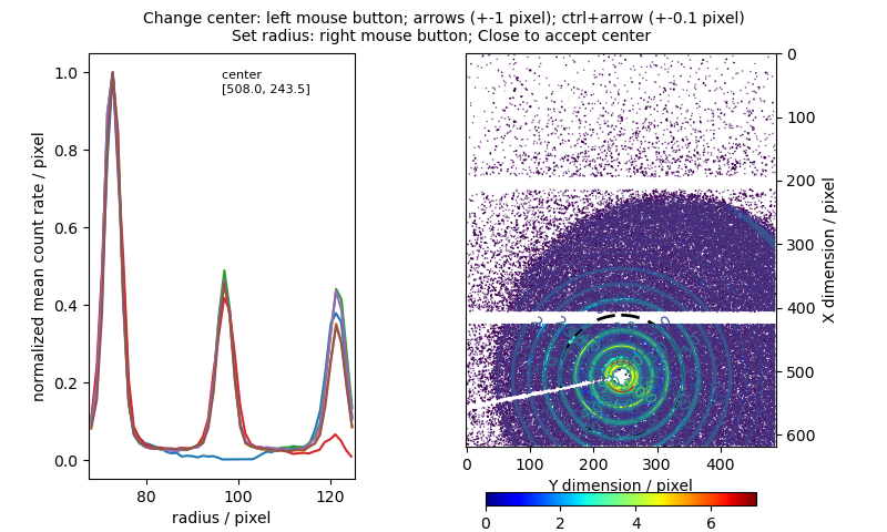
Examples

import jscatter as js
#
calibration = js.sas.sasImage(js.examples.datapath+'/calibration.tiff')
# use pickBeamcenter
calibration.pickBeamcenter()

radialAverage(center=None, number=300, kind='log', calcError=False, units=None)

Radial average of image and conversion to wavevector q.

Remember to set .detector_distance to calibrated value. Setting units to ‘sr’ will scale the output to counts/micro_steradians which also accounts for different detector distances.

Parameters:

centerlist 2x float

Sets center in data and uses this. If not given the attributecenter in the data is used.

numberint, default 500

Number of intervals on new X scale.

kind‘lin’, ‘log’, array default ‘log’

Determines how points are distributed on the Q scale. (See dataArray.prune) It may be an array with an explicit list from another radialAveraged image (like im.radialAverage(…).X) . If the images have different centers then some intervals around the center might be empty. These are filled with interpolated values. Just avoid different centers.

calcError‘poisson’,’std’, default None

How to calculate error.

• ‘poisson’ according to Poisson statistics.

  Use for original images showing unprocessed photon/neutron counts. E.g for Dectris detectors or SANS detectors, but not for CCD cameras.

• ‘std’ as standard deviation of the values in an interval.

• otherwise no error

unitsNone, ‘sr’

Units of the returned radial average as :

• None default counts per pixel

• ‘sr’ counts per solid angle as counts/micro steradians = 1e-6 counts/steradians. This accounts also different detector distances.

Returns:

dataArray with added attributes of the image. artist and entriesXML are ommited

Notes

• Correction of pixel size for flat detector projected to Ewald sphere included. The correction is relative to the pixel located at the center. The intensity remains in units counts/pixel.

• The value in a q binning is the average count rate \(c(q)=(\sum c_i)/N\) with counts in pixel i \(c_i\) and number of pixels \(N\)

• Setting units to ‘sr’ scales to counts per solid angle (micro steradians). In these units the scattered intensity is independent of the detector distance. Scaling is done after calculation of the error.

• calcError : If the image is unprocessed (no background subtraction or transmission correction) containing original photon count rates the standard error can be calculated from Poisson statistic.

  • The error (standard deviation) is calculated in a q binning as \(e=(\sum c_i)^{1/2}/N\)

  • The error is valid for single photon counting detectors showing Poisson statistics as the today typical Pilatus detectors from DECTRIS.

  • The error for \(\sum c_i) <= 0\) is set to zero. One may estimate the corresponding error from neighboring intervals.

  • In later 1D processing as e.g. background correction the error can be included according to error propagation.

  ‘std’ calcs the error as standard deviation in an interval.

Examples

For Pilatus detector including some average with less pixel at high Q I use

sample = image.radialAverage(kind='log',number=200, calcError='poisson',units='sr').prune(0.1,6)

Mask and do radial average over sectors.

import jscatter as js
cal = js.sas.sasImage(js.examples.datapath+'/calibration.tiff')
p=js.grace()
calc=cal.copy()
calc.maskSectors([0,180],20,radialmax=100,invert=True)
calc.show()
icalc=calc.radialAverage()
p.plot(icalc,le='horizontal')
calc=cal.copy()
calc.maskSectors([90+0,90+180],20,radialmax=100,invert=True)
calc.show()
icalc=calc.radialAverage()
p.plot(icalc,le='vertical')
p.yaxis(scale='l')
p.legend()
p.title('The AgBe is not isotropically ordered')

recalibrateDetDistance(center=None, number=500, fcenter=1.0, fwhm=0.1, peaks=None, showfits=False)

Recalibration of detectorDistance by AgBe reference for point collimation.

Use only for AgBe reference measurements to determine the correction factor. For non AgBe measurements set during reading or .detector_distance to the new value. May not work if the detector distance is totally wrong.

Parameters:

centerlist 2x float

Sets beam center or radial center in data and uses this. If not given the attributecenter in the data is used.

numberint, default 1000

number of intervals on new X scale.

fcenterfloat, default 1

Determines start value for peak fitting.

By default, the position of the peak maximum is used if it is larger than (mean(Y)+2std(Y)) of the signal Y. Otherwise fcenter*peakposition[i] is used. Negative fcenter forces the start value to be |fcenter|*peakposition[i].

Reference peakpositions in 1/nm:

[1.0753, 2.1521, 3.2286, 4.3049, 5.3813, 6.4576, 7.5339, 8.6102, 9.6865, 10.7628]

fwhmfloat, default 0.1

Start value for full width half maximum in peak fitting.

peakslist of float

Peak positions of a reference measurement. By default these are the AgBe peaks. Check `js.sas.AgBepeaks`. Can also be used to limit the used peaks if one is bad or change the reference material.

showfitsbool

Show the AgBe peak fits.

Notes

• .distanceCorrection will contain factor for correction. Repeating this results in a .distanceCorrection close to 1.

• To check the result use showfits=True.

• The fits should all fit well to accept the result. To improve use sasImage.maskCircle() to cover an inside region and with invert=True the outside edges. For bad result try to change the detectordistance to a more reasonable value as first guess. This can be recognized if the AgBe peaks shown with showfits=True are not approximately centered within the data range for fitting.

We fit a Voigt function to each of the detected peaks in the image and use the average of the resulting correction factors for each peak as overall correction factor.

As a background we fit a power law as this is needed on some beam line machines.

reduceSize(bin=2, center=None, border=None)

Reduce size of image using uniform average in box.

Center, pixel_size are scaled correspondingly.

Parameters:

binint

Size of box to average within. Also factor for reduction in image size.

center[int,int]

Center of crop region.

borderint

Size of crop region.

• If center is given a box with 2*size around center is used.

• If center is None the border is cut by size.

Returns:

sasImage

saveAsTIF(filename, fill=None, **params)

Save the sasImage as float32 tif without loosing information.

Conversion from float64 to float32 is necessary. To save colored images use asImage.save() (see asImage())

Parameters:

filenamestring

Filename to save to.

fillfloat, ‘min’ default None

Fill value for masked values. By default this is -1.

‘min’ uses the minimal value of the respective data type

• np.iinfo(np.int32).min = -2147483648 for int32

• np.finfo(np.float32).min = -3.4028235e+38 for float32

paramskwargs

Additional kwargs for PIL.Image.save if needed.

Examples

import jscatter as js
cal = js.sas.sasImage(js.examples.datapath+'/calibration.tiff')
cal2=cal/2.
cal2.saveAsTIF('mycal',fill=-100)
mycal=js.sas.sasImage('mycal.tif',maskbelow=-200)
mycal.show()

setAttrFromImage(image)

Copy center, detector_distance, alpha, beta, gamma wavelength, pixel_size from image.

Parameters:

image sasImage

sasImage to copy attributes to self.

setDetectorDistance(detector_distance)

Set detector distance as shortest distance to sample along plane normal vector.

Parameters:

detector_distancefloat, sasImage

New value for detector distance in units m. If sasImage the detector_distance is copied.

Notes

EXIF data show this as list so we stay to this.

setDetectorPosition(center, detector_distance, alpha=None, beta=None, gamma=None)

Set parameters describing the position and orientation of the detector.

Parameters:

center2x float

Center of the detector where the plane normal is going through the sample origin in pixel units. For conventional small angle scattering geometry (detector plane perpendicular to incoming beam) this is the beam center.

detector_distancefloat

Distance of the detector center to sample origin in units m.

alphafloat

Angle between incident beam and detector plane normal in degree. Or the angle between incident beam and the vector pointing from the sample to the detector center. E.g. 0° for SAS.

betafloat

Rotation angle of detector pixel X dimension around detector plane normal in degree. Determines orientation of detector, rotating the detector in plane.

gammafloat

Rotation of detector normal around incident beam in degree. Position of the detector as seen from sample or like rotating the sample around incident beam.

For Debye-Scherer ring pattern (powder average) equal 0.

setPixelSize(pixel_size)

Set pixel_size.

Parameters:

pixel_size[float,float]

Pixel size in [x,y] direction in units m.

setPlaneCenter(center)

Set beamcenter or center of detector plane where plane normal has shortest distance to sample.

In standard SAS geometry this is equal to the beamcenter. For offset detectors is point of closest distance.

Parameters:

center2x float, sasImage

New value for center as [height, width] coordinates. If sasImage the center is copied.

setPlaneOrientation(alpha=None, beta=None, gamma=None)

Set orientation angles of detector plane .

In standard SAS geometry these are equal 0.

Parameters:

alphafloat

Angle between incident beam and detector plane normal in degree. Or the angle between incident beam and the vector pointing from the sample to the detector center. E.g. 0° for SAS.

betafloat

Rotation angle of detector pixel X dimension around detector plane normal in degree. Determines orientation of detector, rotating the detector in plane.

gammafloat

Rotation of detector normal around incident beam in degree. Position of the detector as seen from sample or like rotating the sample around incident beam.

For Debye-Scherer ring pattern (powder average) equal 0.

setWavelength(wavelength)

Set wavelength.

Parameters:

wavelength[float]

Wavelength in units angstrom.

show(**kwargs)

Show sasImage as matplotlib figure.

Parameters:

scale‘log’, ‘symlog’, default = ‘norm’

Scale for intensities.

• ‘norm’ Linear scale.

• ‘log’ Logarithmic scale

• ‘symlog’ Symmetrical logarithmic scale is logarithmic in both the positive and negative directions from the origin. This works also for only positive data. Use linthresh, linscale to adjust.

levelsint, None

Number of contour levels.

colorMapstring

Get a colormap instance from name. Standard mpl colormap name (see showColors).

badcolorfloat, color

Set the color for bad values (like masked) values in an image. Default is bad values be transparent. Color can be matplotlib color as ‘k’,’b’ or float value in interval [0,1] of the chosen colorMap. 0 sets to minimum value, 1 to maximum value.

linthreshfloat, default = 1

Only used for scale ‘symlog’. The range within which the plot is linear (-linthresh to linthresh).

linscalefloat, default = 1

Only used for scale ‘symlog’. Its value is the number of decades to use for each half of the linear range. E.g. 10 uses 1 decade.

lineMapstring

Label color Colormap name as in colorMap, otherwise as cs in in Axes.clabel * if None, the color of each label matches the color of the corresponding contour * if one string color, e.g., colors = ‘r’ or colors = ‘red’, all labels will be plotted in this color * if a tuple of matplotlib color args (string, float, rgb, etc),

different labels will be plotted in different colors in the order specified

fontsizeint, default 10

Size of line labels in pixel

axisNone, ‘pixel’

If coordinates should be forced to pixel, otherwise wavevectors if possible.

invert_yaxis, invert_xaxisbool

Invert corresponding axis.

blockbool

Open in blocking or non-blocking mode

origin‘lower’,’upper’

Origin of the plot. See matplotlib imshow.

Returns:

image handle

Notes

To show data as Image in correct orientation the option ax.invert_yaxis() is used. If you plot directly with matplotlib use the same.

Examples

Use radial averaged data to interpolate

import jscatter as js
import numpy as np
calibration = js.sas.sasImage(js.examples.datapath+'/calibration.tiff')
calibration.show(colorMap='ocean')
calibration.show(scale='sym',linthresh=20, linscale=5)

Use scale='symlog' for mixed lin-log scaling to pronounce low scattering. See mpl.contourImage for more options also available using .show.

import jscatter as js
import numpy as np
# sets negative values to zero
bsa = js.sas.sasImage(js.examples.datapath+'/BSA11mg.tiff')
fig=js.mpl.contourImage(bsa,scale='sym',linthresh=30, linscale=10)
fig.axes[0].set_xlabel(r'$Q_{{ \mathrm{{X}} }}\;/\;\mathrm{{nm^{{-1}}}}$ ')
fig.axes[0].set_ylabel(r'$Q_{{ \mathrm{{Y}} }}\;/\;\mathrm{{nm^{{-1}}}}$ ')

showPolar(center=None, scaleR=1, offset=0, scale='log')

Show image transformed to polar coordinates around center.

Azimuth for standard SAS geometry corresponds to: center line upwards, upper quarter center to right upper/lower edge = center downwards, lower quarter center to left

Parameters:

center[int,int]

Beamcenter

scaleRfloat

Scaling factor for radial component to zoom the center. Works only for alpha,beta,gamma = 0 .

offsetfloat

Offset to remove center from polar image. Works only for alpha,beta,gamma = 0 .

scale‘log’, ‘symlog’, default = ‘log’

Scale for intensities.

• ‘norm’ Linear scale.

• ‘log’ Logarithmic scale

• ‘symlog’ Symmetrical logarithmic scale is logarithmic in both the positive and negative directions from the origin. This works also for only positive data. Use linthresh, linscale to adjust.

Returns:

Handle to figure

Examples

Use polar coordinates to see if center is in middle of Debye-Scherrer rings. First standard SAS geometry:

import jscatter as js
calibration = js.sas.sasImage(js.examples.datapath+'/calibration.tiff')
calibration.showPolar()

For offset detector

import jscatter as js
import numpy as np

sic = js.sas.sasImage(js.examples.datapath+'/Silicon.tiff')
sic.setDetectorPosition([130,-100],0.070,90,90,0)
sic.showPolar()

jscatter.sas.shortprint(values, threshold=6, edgeitems=2)

Creates a short handy representation string for array values.

Parameters:

valuesobject

Values to print.

threshold: int default 6

Number of elements to switch to reduced form.

edgeitemsint default 2

Items at the edge.

jscatter.sas.simpson(y, x=None, *, dx=1.0, axis=-1)

Integrate y(x) using samples along the given axis and the composite Simpson’s rule. If x is None, spacing of dx is assumed.

Parameters:

yarray_like

Array to be integrated.

xarray_like, optional

If given, the points at which y is sampled.

dxfloat, optional

Spacing of integration points along axis of x. Only used when x is None. Default is 1.

axisint, optional

Axis along which to integrate. Default is the last axis.

Returns:

float

The estimated integral computed with the composite Simpson’s rule.

See also

quad()

adaptive quadrature using QUADPACK

fixed_quad()

fixed-order Gaussian quadrature

dblquad()

double integrals

tplquad()

triple integrals

romb()

integrators for sampled data

cumulative_trapezoid()

cumulative integration for sampled data

cumulative_simpson()

cumulative integration using Simpson’s 1/3 rule

Notes

For an odd number of samples that are equally spaced the result is exact if the function is a polynomial of order 3 or less. If the samples are not equally spaced, then the result is exact only if the function is a polynomial of order 2 or less.

Array API Standard Support

simpson has experimental support for Python Array API Standard compatible backends in addition to NumPy. Please consider testing these features by setting an environment variable SCIPY_ARRAY_API=1 and providing CuPy, PyTorch, JAX, or Dask arrays as array arguments. The following combinations of backend and device (or other capability) are supported.

Library	CPU	GPU
NumPy	✅	n/a
CuPy	n/a	✅
PyTorch	✅	✅
JAX	✅	✅
Dask	✅	n/a

See dev-arrayapi for more information.

References

[1]

Cartwright, Kenneth V. Simpson’s Rule Cumulative Integration with MS Excel and Irregularly-spaced Data. Journal of Mathematical Sciences and Mathematics Education. 12 (2): 1-9

Examples

>>> from scipy import integrate
>>> import numpy as np
>>> x = np.arange(0, 10)
>>> y = np.arange(0, 10)

>>> integrate.simpson(y, x=x)
40.5

>>> y = np.power(x, 3)
>>> integrate.simpson(y, x=x)
1640.5
>>> integrate.quad(lambda x: x**3, 0, 9)[0]
1640.25

jscatter.sas.smear(unsmeared=None, *, beamProfile=None, **smkwargs)

Smearing model/data for point collimation SANS/SAXS or line-collimated SAXS (Kratky camera) allowing simultaneous SAXS/SANS fitting.

The beamProfile parameter has to be given as keyword argument beamProfile=mybeam.

Smearing at detector edges involves evaluation of the model at extrapolated q values.

• For model functions smear is used as decorator @smear and the q range is automatically extended.

• Simultaneous fitting of SAXS/SANS (inclusive multiple detector distances) the data need corresponding .beamProfile as attribute. During fitting .beamprofile is used for smearing of the model. See Notes for usage.

• For explicit given data extrapolation at each edge needs to be chosen according to the observed behavior at the edge (eg power law at low q or constant at high q). See prepareBeamProfile for the options.

Call only with keyword arguments. See Notes for details.

Parameters:

unsmearedfunction or dataArray

Model function or explicit data to be smeared. The scattering vector in the model function should have name starting with one of ‘qQ’. If used as a decorator the function is inserted automatically by the @smear syntax and should not be given. If any smearing related parameter is None as detDist=None smearing is bypassed. The unit of Q must be 1/nm

beamProfilebeamProfile or ‘trap’, ‘SANS’, ‘explicit’, dataArray

Beamprofile that determines smearing as prepared from prepareBeamProfile. Always use as keyword argument If no beamProfile is given input and smkwargs are used in prepareBeamProfile to define beamprofile. Measured Profile is also treated by prepareBeamProfile. For explicit profile the width unit must be 1/nm.

smkwargs

See prepareBeamProfile for kwargs.

Returns:

dataArray

• for line collimation: smeared data

• other: dataArray with columns

  [q, smeared data, original data, half width smearing function] and additional attributes as defined in the respective beamProfiles and smeared model.

Notes

Smearing a model function as decorator (like @smear ) for fitting.

Decorators modify functions. Here the model is smeared according to the provided beamprofile extending the q range at edges.

The model scattering vector must have a name starting with one of “qQ”. Units for Q is 1/nm.

• Beamprofile parameters as detDist are updated for smearing during the function call. This allows that during fitting also beamprofile parameters can be fitted. Setting any of the beamprofile parameters to None bypasses smearing (e.g. for SAXS or simulation).

  Use as :

  # define resolution
  resol2m = js.sas.prepareBeamProfile('SANS', detDist=2000,collDist=2000.,wavelength=0.4,wavespread=0.10,
                                      collAperture=10, sampleAperture=6, dpixelWidth=10, dringwidth=1)
  
  # decorate model to automatically smear it (dont use `unsmeared` argument as it is added automatically)
  @js.sas.smear(beamProfile=resol2m)
  def smearedSphere(q,R,bgr,detDist=3000,collDist=2000.,c=1):
      sp = js.ff.sphere(q=q,radius=R,contrast=c)
      sp.Y=sp.Y+bgr
      return sp
  
  # for fitting with attribute detDist and collDist in fitted data for different detector distances
  sp=smearedSphere(q=q,R=13,detDist=8000,collDist=8000.)
  

  The above decorator is equivalent to the following. Use smearedSphere as smeared model function.

  def sphere(q,R,bgr,detDist=3000,collDist=2000.,contrast=1):
      sp = js.ff.sphere(q,R,contrast)
      sp.Y=sp.Y+bgr
      return sp
  smearedsphere=js.sas.smear(sphere,beamProfile=resol2m)
  

• To fit SAXS and SANS data together (also with changing beamprofile parameters as collimation) use the parameter beamProfile in the model. If calling the smeared model with a valid beamProfile this is used instead of the one defined in @smear One may remind that also pinhole SAXS has a smearing even if it is small. Ask your instrument responsible for reasonable values or do a measurement of the primary beam.

  This allows fitting with different profiles if the corresponding data contain .beamProfile as attribute. See Fitting multiple smeared data together.

  fbeam = js.sas.prepareBeamProfile(0.02)
  fbeam2 = js.sas.prepareBeamProfile(0.01)
  
  # define smeared model with beamProfile as parameter
  @js.sas.smear(beamProfile=fbeam)
  def sphere(q,R,bgr,contrast=1, beamProfile=None):
      sp = js.ff.sphere(q=q,radius=R,contrast=contrast)
      sp.Y=sp.Y+bgr
      return sp
  
  # call as
  sphere(q=q,R=13,bgr=0,beamProfile=fbeam2)
  
  # to fit data add corresponding beamProfile attribute to each dataArray in a dataList
  dll[0].beamProfile=fbeam
  dll[1].beamProfile=fbeam2
  dll.fit(sphere,.....)
  

• Using merged data (multiple detector distances in one set of data with overlap) is possible with ‘explicit’ beamProfile if (in particular in the overlap region):

  • no q value is used twice

  • for each value a resolution width exists

  • The resolution width is given in same units as q.

  Only this guarantees that always the correct width is used (depending on detector distance). Usually this is fulfilled if you prepare the beamProfile with data containing the width as last column like merged SANS data.

Smear explicit data

Explicit data show artifacts due to smearing at the edges if extrapolation is done wrong. The default is a constant value from the edge which is good for a low q plateau or a high q flat background. For the above model smearing this is not important as the q range is automatically extended. For desmearing e.g. of multi detector distance SANS data this is important if detector edges are within a non constant region.

import jscatter as js
#define beamprofile
resol8m = js.sas.prepareBeamProfile('SANS', detDist=8000,collDist=8000.,wavelength=0.4,wavespread=0.10,
                                    collAperture=15, sampleAperture=5, dpixelWidth=10, dringwidth=1,)
resol8m2 = js.sas.prepareBeamProfile('SANS', detDist=8000,collDist=8000.,wavelength=0.4,wavespread=0.10,
                                    collAperture=15, sampleAperture=5, dpixelWidth=10, dringwidth=1,
                                    extrapolfunc=['guinier',None])
# create some data
q=js.loglist(0.01,1,300)
sp=js.ff.sphere(q,radius=13)
#  smear data
spsmeared=js.sas.smear(sp,beamProfile=resol8m)
# smear in a limited range, default is extrapolation with constant edge value
spsmeared2=js.sas.smear(sp[:,sp.X>0.2],beamProfile=resol8m)
# guinier like extrapolation
spsmeared2ex=js.sas.smear(sp[:,sp.X>0.2],beamProfile=resol8m2)

# plot it
p=js.grace(1,1)
p.plot(sp)
p.plot(spsmeared,li=[1,3,1],sy=0)
p.plot(spsmeared2,li=[1,3,2],sy=0,le='low edge underestimate')
p.plot(spsmeared2ex,li=[1,3,3],sy=0,le='low edge improved')
p.yaxis(scale='log',min=10000,max=1e8)
p.legend(x=0.2,y=1e5)
p.new_graph(xmin=0.5,xmax=0.9,ymin=0.55,ymax=0.9)
xs=(spsmeared.X>0.18) & (spsmeared.X<0.25)
p[1].plot(spsmeared[:,xs],li=[1,3,1],sy=0)
xs=(spsmeared2.X>0.18) & (spsmeared2.X<0.25)
p[1].plot(spsmeared2[:,xs],li=[1,3,2],sy=0)
p[1].plot(spsmeared2ex[:,xs],li=[1,3,3],sy=0)
p[1].yaxis(scale='log',min=8e6,max=2e7)
p[0].title('Examine smearing at edge')

• If unsmeared has attributes a, b, dIW, bxw, detDist these are used for the beamProfile, if not given in function call.

• If wavelength is missing in data a default of 0.155418 nm for Xray \(K_{\alpha}\) line is assumed. For SANS 0.5 nm.

• During smearing for Kratky camera an integration over the beam width and beam length are performed. In this integration \(q_{w,l}= ((q+q_{w})^2)+q_{l}^2)^{1/2}\) is used with \(q_{w}\) along the beam width and \(q_{l}\) along the beam length. in regions \(q_{w,l} > max(q_{data})\) we estimate the measured scattering intensity by the mean of the last 10 points of the measured spectra to allow for a maximum in \(q\) range. The strictly valid q range can be estimated by calculating \(q_{x,y} < max(q)\) with 2 times the used beam width and beam length. As the smearing for larger \(q\) has no real effect the estimate might be still ok.

Examples

For more examples see How to build a more complex model, How to fit SANS data including the resolution for different detector distances and Smearing and desmearing of SAX and SANS data.

import jscatter as js
q=js.loglist(0.01,4,300)

def sphere(q,R,bgr,contrast=1):
    sp = js.ff.sphere(q,R,contrast)
    sp.Y=sp.Y+bgr
    return sp
#
# prepare different beamprofiles
# measured Kratky camera BeamProfile.pdh for line collimation
beam = js.sas.readpdh(js.examples.datapath+'/BeamProfile.pdh')
mbeam = js.sas.prepareBeamProfile(beam , bxw=0.01, dIW=1.)
#
# Kratky camera with explicit given beamprofile parameters describing trapezoidal beam profile
tbeam = js.sas.prepareBeamProfile('trapez', a=mbeam.a, b=mbeam.b, bxw=0.01, dIW=1)
#
# different SANS detector distances, see  prepareBeamProfile for default parameters
Sbeam1 = js.sas.prepareBeamProfile('SANS', detDist=2000,wavelength=0.4,wavespread=0.1,sampleAperture=5)
Sbeam2 = js.sas.prepareBeamProfile('SANS', detDist=20000,wavelength=0.4,wavespread=0.1,sampleAperture=5)
#
# Using an explicit given resolution width in column 3
# here q and resolution width (column 3) must have units 1/nm
i70=js.dL(js.examples.datapath+'/polymer.dat')[0]
Gbeam = js.sas.prepareBeamProfile(i70,explicit=3)
#
# Using a single width e.g. for point collimation SAXS data
# the width corresponds to Gaussian width from attenuated empty beam measurement
fbeam = js.sas.prepareBeamProfile(0.01)

# smear data
data = sphere(q,R=25,bgr=1000)
datasm = js.sas.smear(unsmeared=data,beamProfile=mbeam)
datast = js.sas.smear(unsmeared=data,beamProfile=tbeam)
datasS1 = js.sas.smear(unsmeared=data,beamProfile=Sbeam1)
datasS2 = js.sas.smear(unsmeared=data,beamProfile=Sbeam2)
datasG = js.sas.smear(unsmeared=data,beamProfile=Gbeam)
datasf = js.sas.smear(unsmeared=data,beamProfile=fbeam)

p=js.grace()
p.title('resolution smearing in small angle scattering')
p.plot(data,li=[1,2,-1],sy=0,le='unsmeared')
for dat in [datasm,datast,datasS1,datasS2,datasG,datasf]:
   p.plot(dat,li=[1,2,-1],sy=0,le=dat.beamProfile.beamProfType)
p.yaxis(scale='l')
p.xaxis(scale='l')
p.legend(x=1,y=1e8)
p.text(r'Kratky camera \nline collimation' , x=0.02,y=2e7)
p.text('point collimation' , x=0.2,y=8e8)
p.xaxis(label=r'Q / nm\S-1')
p.yaxis(label=r'I(Q) / a.u.')
#p.save(js.examples.imagepath+'/smearingexamples.png')

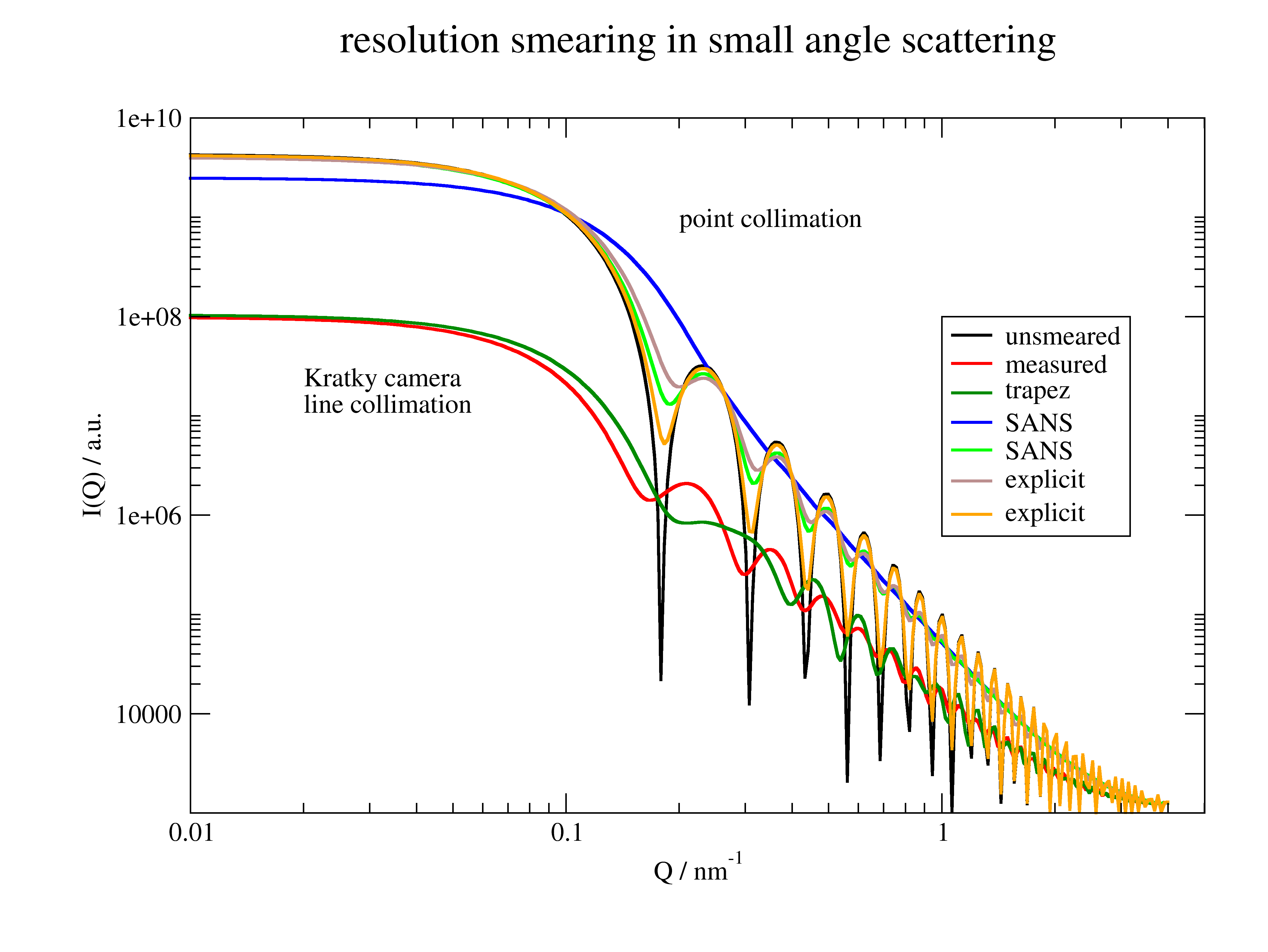
jscatter.sas.smooth(data, windowlen=7, window='flat')

Smooth data by convolution with window function or fft/ifft.

Smoothing based on position ignoring information on .X.

Parameters:

dataarray, dataArray

Data to smooth. If is dataArray the .Y is smoothed and returned.

windowlenint, default = 7

The length/size of the smoothing window; should be an odd integer. Smaller 3 returns unchanged data. For ‘fourier’ the high frequency cutoff is 2*size_data/windowlen.

window‘hann’, ‘hamming’, ‘bartlett’, ‘blackman’,’gaussian’,’fourier’,’flattop’ default =’flat’

Type of window/smoothing.

• ‘flat’ will produce a moving average smoothing.

• ‘gaussian’ normalized Gaussian window with sigma=windowlen/7.

• ‘fourier’ cuts high frequencies above cutoff frequency between rfft and irfft.

Returns:

array (only the smoothed array)

Notes

‘hann’, ‘hamming’, ‘bartlett’, ‘blackman’,’gaussian’, ‘flat’ :

These methods convolve a scaled window function with the signal. The signal is prepared by introducing reflected copies of the signal (with the window size) at both ends so that transient parts are minimized in the beginning and end part of the output signal. Adapted from SciPy/Cookbook.

See https://docs.scipy.org/doc/scipy-1.11.0/reference/generated/scipy.signal.get_window.html#scipy.signal.get_window

fourier :

The real valued signal is mirrored at left side, Fourier transformed, the high frequencies are cut and the signal is back transformed. This is the simplest form as a hard cutoff frequency is used (ideal low pass filter) and may be improved using a specific window function in frequency domain.

rft = np.fft.rfft(np.r_[data[::-1],data])
rft[int(2*len(data)/windowlen):] = 0
smoothed = np.fft.irfft(rft)

Examples

Usage:

import jscatter as js
import numpy as np
t=np.r_[-5:5:0.01]
data=np.sin(t)+np.random.randn(len(t))*0.1
y=js.formel.smooth(data)  # 1d array
#
# smooth dataArray and replace .Y values.
data2=js.dA(np.vstack([t,data]))
data2.Y=js.formel.smooth(data2, windowlen=40, window='gaussian')

Comparison of some filters:

import jscatter as js
import numpy as np
t=np.r_[-5:5:0.01]
data=js.dA(np.vstack([t,np.sin(t)+np.random.randn(len(t))*0.1]))
p=js.grace()
p.multi(4,2)
windowlen=31
for i,window in enumerate(['flat','gaussian','hann','fourier']):
    p[2*i].plot(data,sy=[1,0.1,6],le='original + noise')
    p[2*i].plot(t,js.formel.smooth(data,windowlen,window),sy=[2,0.1,4],le='filtered')
    p[2*i].plot(t,np.sin(t),li=[1,0.5,1],sy=0,le='noiseless')
    p[2*i+1].plot(data,sy=[1,0.1,6],le='original noise')
    p[2*i+1].plot(t,js.formel.smooth(data,windowlen,window),sy=[2,0.1,4],le=window)
    p[2*i+1].plot(t,np.sin(t),li=[1,2,1],sy=0,le='noiseless')
    p[2*i+1].text(window,x=-2.8,y=-1.2)
    p[2*i+1].xaxis(min=-3,max=-1,)
    p[2*i+1].yaxis(min=-1.5,max=-0.2,ticklabel=[None,None,None,'opposite'])
    p[2*i].yaxis(label='y')
p[0].legend(x=10,y=4.5)
p[6].xaxis(label='x')
p[7].xaxis(label='x')
p[0].title(f'Comparison of smoothing windows')
p[0].subtitle(f'with windowlen {windowlen}')
#p.save(js.examples.imagepath+'/smooth.jpg')

jscatter.sas.subarray

alias of SubArray

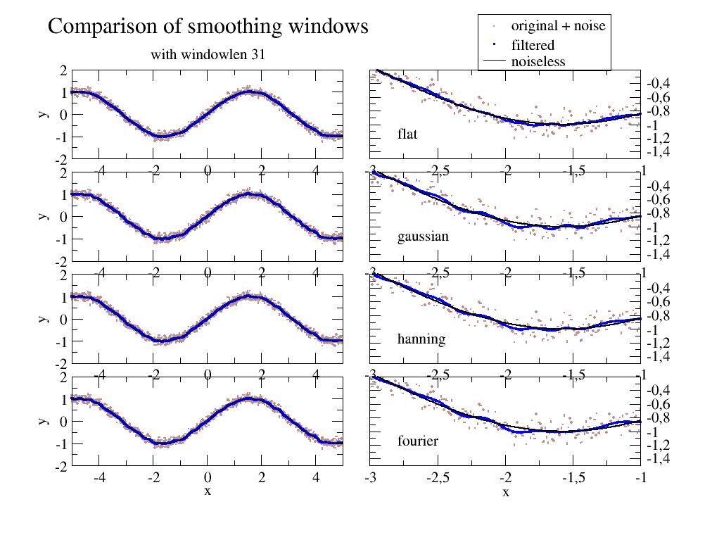
jscatter.sas.transmissionCorrection(data, dark=None, emptybeam=None, edge=0.03, exposure=None, transmission=None, Izero=None)

Subtract dark current, find primary beam, get transmission count and normalize by transmission and exposure time. IN PLACE.

For measurements including the primary beam (no beamstop or from semitransparent beamstop) or with explicit given parameters. The maximum of the primary beam peak after dark subtraction determines transmission counts for the first.

Parameters:

datadataArray

A raw measurement

• From a SAXSpace instrument read by js.dA(‘filename.pdh’,lines2parameter=[2,3,4]) including primary beam.

• From a SAXSpace measurement read as sasImage and averaged using image.lineAverage including primary beam and background subtracted (use dark = None).

• Ganesha radial averaged data with additional parameters.

• For other data the missing parameters need to be given explicitly.

darkdataArray, None

Dark current measurement \(I_{dark}\).

• None,0: Dark is already subtracted.

• dataArray: A dark measurements including dead pixel. (these are corrected doing the subtraction).

• float: Dark as counts/pixel/s. E.g. a value <0.1/3600s for Dectris detectors as noted in the datasheet.

emptybeamdataArray, float, default=None

Empty beam measurement \(I_b\) to subtract from measurement.

• If it is a raw measurement (not transmission corrected) first transmissionCorrection is applied. emptybeam.transmission==1 and .primarypeakmean is given in units (counts/s).

• If float (in units counts/s) this value is used as emptybeam.primarypeakmean for calculation of the actual sample transmission.

edgefloat, default 0.03

Wavevector value below beam stop edge. Also the primary beam is searched below this value.

exposureoptional, float, default None

Exposure time \(t_{exposure}\) in unit ‘s’. If not given explicit it is extracted from the data :

• For SAXSpace data the xml description at the end of the file is examined.

• For Ganesha data from .exposure_time[0]

transmissionoptional, float, str, None

Transmission T of the data measurement.

• float: explicitly given transmission T.

• ‘edge’: detect as average below edge.

• If primary beam is included (SAXSpace) from the peak height.

• From Ganesha data from entry .transmission_factor[0]

Izerofloat, None

Intensity primary beam \(I_0\) for normalisation if different detector distances are used.

• For Ganesha measurements taken from .Izero[0] (units counts/s).

• Ignored for SAXSpace Izero=1.

Returns:

None, IN PLACE

• Adds attributes .centerTransmissionPeak, .centerTransmissionPeakMax and .transmission as relative transmission to primary beam for samples for SAXSSpace.

• If emptybeam is NOT given the transmission value is the maximum peak value in counts/s. The same is for evaluating the emptybeam measurement itself. To compare the treated emptybeam multiply with this maximum peak value.

Notes

After using transmissionCorrection the data contain (also in given emptybeam)

\(I' = \big(\frac{I-I_{dark}}{T}-I_{b}T\big) /I_0/t_{exposure}\)

Correction

Brulet at al [1] describe the data correction for SANS, which is in principle also valid for SAXS, if incoherent contributions are neglected.

The difference is, that SAXS has typical transmission around ~0.3 for 1mm water sample in quartz cell due to absorption, while in SANS typical values are around ~0.9 for D2O. Larger volume fractions in the sample play a more important rule for SANS as hydrogenated ingredients reduce the transmission significantly, while in SAXS still the water and the cell (quartz) dominate.

One finds for a sample inside of a container with thicknesses (\(z\)) for sample, buffer (solvent), empty cell and empty beam measurement (omitting the overall q dependence):

\[I_s = \frac{1}{z_S}\big((\frac{I_S-I_{dark}}{T_S}-I_{b}T_S\big) - \big(\frac{I_{EC}-I_{dark}}{T_{EC}}-I_{b}T_{EC})\big) - \frac{1}{z_B}\big((\frac{I_B-I_{dark}}{T_B}-I_{b}T_B\big) - \big(\frac{I_{EC}-I_{dark}}{T_{EC}}-I_{b}T_{EC})\big)\]

where

• \(I_s\) is the interesting species

• \(I_S\) is the sample of species in solvent (buffer)

• \(I_B\) is the pure solvent (describing a constant background)

• \(I_{dark}\) is the dark current measurement

• \(I_b\) is the empty beam measurement

• \(I_{EC}\) is the empty cell measurement

• \(z_x\) corresponding sample thickness

• \(T_x\) corresponding transmission as primary beam intensity ratio \(T_x=I_x(0)/I_b(0)\)

The recurring pattern \(\big((\frac{I-I_{dark}}{T}-I_{b}T\big)\) shows that the primary beam (not absorbed by the beam stop) is attenuated by the corresponding sample contributing unscattered intensity.

For equal sample thickness \(z\) the empty beam is included in subtraction of \(I_B\):

\[I_s = \frac{1}{z} \big((\frac{I_S-I_{dark}}{T_S}-I_{b}T_S) - (\frac{I_B-I_{dark}}{T_B}-I_{b}T_B)\big)\]

The simple case

If the transmissions are nearly equal as for e.g. protein samples with low concentration (\(T_S \approx T_B\)) we only need to subtract the transmission and dark current corrected buffer measurement from the sample.

\[I_s = \frac{1}{z} \big((\frac{I_S-I_{dark}}{T_S}) - (\frac{I_B-I_{dark}}{T_B}\big)\]

Higher accuracy for large volume fractions

For larger volume fractions \(\Phi\) the transmission might be different and we have to take into account that only \(1-\Phi\) of solvent contributes to \(I_S\). We may incorporate this in the sense of an optical density changing the effective thickness \(\frac{1}{z_B}\rightarrow\frac{1-\Phi}{z_B}\) resulting in different thicknesses \(z_S \neq z_B\)

Transmission

The transmission is measured as the ratio \(T=\frac{I(q=0)_{sample}}{I(q=0)_{emptybeam}}\) with \(I(q=0)\) as the primary beam intensity.

If the primary beam tail is neglected in the above equation \(I(q=0)_{emptybeam}\) only gives a common scaling factor and can be omitted if arbitrary units are used. Alternatively one can scale to the EC transmission with \(T_{EC}=1\) For absolute calibration the same needs to be done. One finds \(T_{sample in cell}=T_{empty cell}T_{sample without cell}\).

References

[1]

Improvement of data treatment in small-angle neutron scattering Brûlet et al.Journal of Applied Crystallography 40, 165-177 (2007)

jscatter.sas.trapezoid(y, x=None, dx=1.0, axis=-1)

Integrate along the given axis using the composite trapezoidal rule.

If x is provided, the integration happens in sequence along its elements - they are not sorted.

Integrate y (x) along each 1d slice on the given axis, compute \(\int y(x) dx\). When x is specified, this integrates along the parametric curve, computing \(\int_t y(t) dt = \int_t y(t) \left.\frac{dx}{dt}\right|_{x=x(t)} dt\).

Parameters:

yarray_like

Input array to integrate.

xarray_like, optional

The sample points corresponding to the y values. If x is None, the sample points are assumed to be evenly spaced dx apart. The default is None.

dxscalar, optional

The spacing between sample points when x is None. The default is 1.

axisint, optional

The axis along which to integrate. The default is the last axis.

Returns:

trapezoidfloat or ndarray

Definite integral of y = n-dimensional array as approximated along a single axis by the trapezoidal rule. If y is a 1-dimensional array, then the result is a float. If n is greater than 1, then the result is an n-1 dimensional array.

See also

cumulative_trapezoid(), simpson(), romb()

Notes

Image [2] illustrates trapezoidal rule – y-axis locations of points will be taken from y array, by default x-axis distances between points will be 1.0, alternatively they can be provided with x array or with dx scalar. Return value will be equal to combined area under the red lines.

Array API Standard Support

trapezoid has experimental support for Python Array API Standard compatible backends in addition to NumPy. Please consider testing these features by setting an environment variable SCIPY_ARRAY_API=1 and providing CuPy, PyTorch, JAX, or Dask arrays as array arguments. The following combinations of backend and device (or other capability) are supported.

Library	CPU	GPU
NumPy	✅	n/a
CuPy	n/a	✅
PyTorch	✅	✅
JAX	⛔	⛔
Dask	✅	n/a

See dev-arrayapi for more information.

References

[1]

Wikipedia page: https://en.wikipedia.org/wiki/Trapezoidal_rule

[2]

Illustration image: https://en.wikipedia.org/wiki/File:Composite_trapezoidal_rule_illustration.png

Examples

Use the trapezoidal rule on evenly spaced points:

>>> import numpy as np
>>> from scipy import integrate
>>> integrate.trapezoid([1, 2, 3])
4.0

The spacing between sample points can be selected by either the x or dx arguments:

>>> integrate.trapezoid([1, 2, 3], x=[4, 6, 8])
8.0
>>> integrate.trapezoid([1, 2, 3], dx=2)
8.0

Using a decreasing x corresponds to integrating in reverse:

>>> integrate.trapezoid([1, 2, 3], x=[8, 6, 4])
-8.0

More generally x is used to integrate along a parametric curve. We can estimate the integral \(\int_0^1 x^2 = 1/3\) using:

>>> x = np.linspace(0, 1, num=50)
>>> y = x**2
>>> integrate.trapezoid(y, x)
0.33340274885464394

Or estimate the area of a circle, noting we repeat the sample which closes the curve:

>>> theta = np.linspace(0, 2 * np.pi, num=1000, endpoint=True)
>>> integrate.trapezoid(np.cos(theta), x=np.sin(theta))
3.141571941375841

trapezoid can be applied along a specified axis to do multiple computations in one call:

>>> a = np.arange(6).reshape(2, 3)
>>> a
array([[0, 1, 2],
       [3, 4, 5]])
>>> integrate.trapezoid(a, axis=0)
array([1.5, 2.5, 3.5])
>>> integrate.trapezoid(a, axis=1)
array([2.,  8.])

jscatter.sas.voigt(x, center=0, fwhm=1, lg=1, asym=0, amplitude=1)

Voigt function for peak analysis (normalized).

The Voigt function is a convolution of gaussian and lorenzian shape peaks for peak analysis. The Lorenzian shows a stronger contribution outside FWHM with a sharper peak. Asymmetry of the shape can be added by a sigmoidal change of the FWHM [2].

Parameters:

xarray

Axis values.

centerfloat

Center of the distribution.

fwhmfloat

Full width half maximum of the Voigt function.

lgfloat, default = 1

Lorenzian/gaussian fraction of both FWHM, describes the contributions of gaussian and lorenzian shape.

• lorenzian/gaussian >> 1 lorenzian,

• lorenzian/gaussian ~ 1 central part gaussian, outside lorenzian wings

• lorenzian/gaussian << 1. gaussian

asymfloat, default=0

Asymmetry factor in sigmoidal as \(fwhm_{asym} = 2*fwhm/(1+np.exp(asym*(x-center)))\) . For a=0 the Voigt is symmetric.

amplitudefloat, default = 1

amplitude

Returns:

dataArray

• .center

• .sigma

• .gamma

• .fwhm

• .asymmetry

• .lorenzianOverGaussian (lg)

Notes

The Voigt function is a convolution of Gaussian and Lorentz functions

\[G(x;\sigma) = e^{-x^2/(2\sigma^2)}/(\sigma \sqrt{2\pi})\ and \ L(x;\gamma) = \gamma/(\pi(x^2+\gamma^2))\]

resulting in

\[V(x;\sigma,\gamma)=\frac{\operatorname{Re}[w(z)]}{\sigma\sqrt{2 \pi}}\]

with \(z=(x+i\gamma)/(\sigma\sqrt{2})\) and \(Re[w(z)]\) is the real part of the Faddeeva function.

\(\gamma\) is the Lorentz fwhm width and \(fwhm=(2\sqrt{2\ln 2})\sigma\) the Gaussian fwhm width.

The FWHM in Lorentz and Gaussian dependent on the fwhm of the Voigt function is \(fwhm_{Gauss,Lorentz} \approx fwhm / (0.5346 lg + (0.2166 lg^2 + 1)^{1/2})\) (accuracy 0.02%).

References

[1]

https://en.wikipedia.org/wiki/Voigt_profile

[2]

A simple asymmetric lineshape for fitting infrared absorption spectra Aaron L. Stancik, Eric B. Brauns Vibrational Spectroscopy 47 (2008) 66–69

[3]

Empirical fits to the Voigt line width: A brief review Olivero, J. J.; R. L. Longbothum Journal of Quantitative Spectroscopy and Radiative Transfer. 17, 233–236. doi:10.1016/0022-4073(77)90161-3

jscatter.sas.waterXrayScattering(composition='h2o1', T=293, units='mol')

Absolute scattering of water with components (salt, buffer) at Q=0 as reference for X-ray.

According to [1] a buffer of water with components might be used. Ions need to be given separatly as [‘55.51h2o1’,’0.15Na1’,’0.15Cl1’] for 0.15 M NaCl solution. It is accounted for the temperature dependence of water density and compressibility.

Parameters:

compositionstring

Buffer composition as in scatteringLengthDensityCalc give dissociated ions separatly as [‘1Na’,’1Cl’] with concentration in mol prepended the additional scattering as ionic liquid of the ions in water is taken into account see [1] . mass in g; 1000g water are 55.508 mol

Tfloat

Temperature in °K

units‘mol’

Anything except ‘mol’ prepended unit is mass fraction. ‘mol’ prepended units is mol and mass fraction is calculated as \(mass=[mol] mass_{molecule}\) e.g. 1l Water with 123 mmol NaCl [‘55.508H2O1’,’0.123Na1’,’0.123Cl1’]

Returns:

float: absolute scattering length in Units 1/cm.

Notes

\(I(0)=(\sigma_{water}^2f_e^2 n_{ew}^2 k_B T \chi + \sum_{ci} n_i N_A 1000 n_{ei}^2 f_e^2 )/100\)

with

• \(\sigma_{water}\) water density

• \(\chi\) compressibility

• \(n_{ew}\) number of electrons per water molecule

• \(f_e\) cross section of electron in nm

• \(k_B\) Boltzmann constant

• \(n_i\) concentration component i

• \(n_{ei}\) number of electrons per molecule component i in Mol

• \(\sum_{ci}\) is done for all ions separately if given

For references regarding waterdensity() and watercompressibility() see respective functions in formel.

References

[1] (1,2)

A high sensitivity pinhole camera for soft condensed matter T. Zemb, O. Tache, F. Né, and O. Spalla, J. Appl. Crystallogr. 36, 800 (2003).

[2]

SAXS experiments on absolute scale with Kratky systems using water as a secondary standard Doris Orthaber et al. J. Appl. Cryst. (2000). 33, 218±225

Examples

# pure H2O
js.sas.waterXrayScattering(['55.5h2o1'])  # 0.0164 1/cm
# phosphate buffer
js.sas.waterXrayScattering(['55.5h2o1','0.2na2h1P1O4','0.2na1H1p1o4','0.1h1'])  # 0.0965 1/cm
# 1M NaCl buffer
js.sas.waterXrayScattering(['55.5h2o1','1na1','1cl1'])  # 0.0360 1/cm
# 100mM NaCl buffer
js.sas.waterXrayScattering(['55.5h2o1','0.1na1','0.1cl1'])  # 0.0183 1/cm

jscatter.sas.watercompressibility(d2ofract=1, T=278, units='psnmg')

Isothermal compressibility of H2O and D2O mixtures.

Compressibility \(\kappa\) in units ps²nm/g or in 1/bar. Linear mixture according to d2ofract.

Parameters:

d2ofractfloat, default 1

Fraction D2O

Tfloat, default 278K

Temperature in K

unitsstring ‘psnmg’

ps^2*nm/(g/mol) or 1/bar

Returns:

float

Notes

For the structure factor e.g. of water one finds in agreement to literature

\[S(0) = kT n \kappa = 0.064\]

with thermal energy kT and number density n,

• \(n = 55.5mol/l = 33.42 /nm³\),

• \(kT=300K*1.380649e^{-23} J/K = 414e^{-23} kgm²/s² = 414e^{-26} g nm²/ps²\)

• \(\kappa(300K)=4.625e20 g/nm/ps²\)

References

[1]

Isothermal compressibility of Deuterium Oxide at various Temperatures Millero FJ and Lepple FK Journal of chemical physics 54,946-949 (1971) http://dx.doi.org/10.1063/1.1675024

[2]

Precise representation of volume properties of water at one atmosphere G. S. Kell J. Chem. Eng. Data, 1967, 12 (1), pp 66–69 http://dx.doi.org/10.1021/je60032a018

Examples

import jscatter as js
n = js.formel.waterdensity('h2o1',T=300) * 1000/18 *6.023e23/1e24
ka = js.formel.watercompressibility(T=300)
kT = 300*1.380649e-26
S0 = kT*n*ka  # => 0.06388

jscatter.sas.waterdensity(composition, T=293.15, units='mol', showvalidity=False)

Density of water with inorganic substances (salts).

Solvent with composition of H2O and D2O and additional inorganic components at temperature T. Ternary solutions allowed. Units are mol

Parameters:

compositionlist of compositional strings

Compositional string of chemical formula as ‘float’+’chemical char’ + integer - First float is content in mol (is later normalized to sum of contents) - chemical letter + number of atoms in formula (single atoms append 1 ,fractional numbers allowed)

'h2o1' or 'd2o1' light and heavy water with 'd1' for deuterium
'c3h8o3' or 'c3h1d7o3' partial deuterated glycerol
['55.55h2o1','2.5Na1Cl1'] for 2.5 mol NaCl added to  1l h2o (55.55 mol)
['20H2O1','35.55D2O1','0.1Na1Cl1'] h2o/d2o mixture with 100mMol NaCl

unitsdefault=’mol’

Anything except ‘mol’ unit is mass fraction ‘mol’ units is mol and mass fraction is calculated as mass=[mol]*mass_of_molecule e.g. 1l Water with 123mM NaCl [‘55.5H2O1’,’0.123Na1Cl1’]

Tfloat, default=293.15

temperature in K

showvaliditybool, default False

Show additionally validity range for temperature and concentration according to [4]. - Temperature range in °C - concentration in wt % or up to a saturated solution (satd) - error in 1/100 % see [4].

Returns:

float

Density in g/ml

Notes

• D2O maximum density 1.10596 at T=273.15+11.23 K [1] .

• For mixtures of H2O/D2O molar volumes add with an accuracy of about 2e-4 cm**3/mol compared to ~18.015 cm**3/mol molar volume [3].

• Additional densities of binary aqueous solutions [4].

Water number density

# 55.5079 mol with 18.015 g/mol
js.formel.waterdensity('1H2O1', T=273+4)*1000/18.015

References

[1]

The dilatation of heavy water K. Stokland, E. Ronaess and L. Tronstad Trans. Faraday Soc., 1939,35, 312-318 DOI: 10.1039/TF9393500312

[2]

Effects of Isotopic Composition, Temperature, Pressure, and Dissolved Gases on the Density of Liquid Water George S. Kell JPCRD 6(4) pp. 1109-1131 (1977)

[3]

Excess volumes for H2O + D2O liquid mixtures Bottomley G Scott R Australian Journal of Chemistry 1976 vol: 29 (2) pp: 427

[4] (1,2,3)

Densities of binary aqueous solutions of 306 inorganic substances P. Novotny, O. Sohnel J. Chem. Eng. Data, 1988, 33 (1), pp 49–55 DOI: 10.1021/je00051a018

availible components:

h2o1 d2o1
TRIS c4h11n1o3
TABS c8h19n1o6s1

     ag1cl104     ag1n1o3      al1cl3012    al1n3o9      al2s3o12     ba1br2      
 ba1cl2       ba1cl2o6     ba1i2        ba1n2o6      c4h11n1o3    c8h19n1o6s1 
 ca1br2       ca1cl2       ca1i2        ca1n2o6      cd1br2       cd1c12      
 cd1i2        cd1n2o6      cd1so4       co1n2o6      co1s1o4      cs1br1      
 cs1cl1       cs1f1        cs1i1        cs1n1o3      cs2s1o4      cu1cl2      
 cu1n2o6      cu1s1o4      dy1cl3       er1cl3       fe1cl3       fe1s1o4     
 gd1cl3       h1br1        h1cl1        h1cl104      h1i1         h1n1o3      
 h2s1o4       h3b103       h3p1o4       hg1c2n2      hg1cl2       k1ag1c2n2   
 k1al1s2o8    k1br1        k1br1o3      k1cl1        k1cl103      k1cl104     
 k1f1         k1h1c1o3     k1h1s1o4     k1h2p1o4     k1i1         k1i103      
 k1mn1o4      k1n1o2       k1n1o3       k1n3         k1o1h1       k1s1c1n1    
 k1tart1      k2c1o3       k2cr104      k2cr207      k2s1o4       k3co1c6n6   
 k3fe1c6n6    k4fe1c6n6    k4mo1c8n8    la1cl3       li1br1       li1cl1      
 li1cl104     li1i1        li1n1o3      li1o1h1      li2s1o4      mg1br2      
 mg1br206     mg1cl2       mg1cl2o8     mg1i2        mg1n2o6      mg1s1o4     
 mn1cl1       mn1s1o4      n1h3         n1h40x1      n1h4ac1      n1h4al1s2o8 
 n1h4cl1      n1h4cl104    n1h4fe1s2o8  n1h4h1s1o4   n1h4h2p1o4   n1h4i1      
 n1h4n1o3     n2h8ni1s2o8  n2h8s1o4     n2s203       na1ac1       na1br1      
 na1br1o3     na1cl1       na1cl103     na1cl104     na1f1        na1form1    
 na1h1s1o4    na1h2p1o4    na1i1        na1i103      na1k1tart1   na1mn104    
 na1n1o2      na1n1o3      na1n3        na1o1h1      na1ox1       na1s1c1n1   
 na1tart1     na2b407      na2c1o3      na2cr1o4     na2cr207     na2h1p1o4   
 na2mo104     na2s1        na2s103      na2s1o4      na2w104      na3p1o4     
 na4p207      na5p307      nd1cl3       ni1cl2       ni1n2o6      ni1s1o4     
 pb1n2o6      pr1cl3       rb1br1       rb1cl1       rb1f1        rb1i1       
 rb1n1o3      rb2so4       sm1cl3       sr1ac2       sr1br2       sr1br206    
 sr1cl2       sr1i2        sr1n2o6      ti1n1o3      ti2s1o4      u1o2n2o6    
 u1o2s104     yb1cl3       zn1br2       zn1cl2       zn1i2        zn1n2o6     
 zn1s1o1     

jscatter.sas.zeros(*args, **kwargs)

dataArray filled with zeros.

Parameters:

shapeinteger or tuple of integer

Shape of the new array, e.g., (2, 3) or 2.

Returns:

dataArray

Examples

js.zeros((3,20))

Read 2D image files from SAXS cameras and extract the corresponding data.

The sasImage is a 2D array that allows direct subtraction and multiplication (e.g. transmission) respecting given masks in operations. E.g.

sample=js.sas.sasImage('sample.tiff')
solvent=js.sas.sasImage('solvent.tiff')
corrected = sample/sampletransmission - solvent/solventtransmission

• Image manipulation like Gaussian filter from scipy.ndimage can be used.

• Calibration of detector distance including offset detector positions, radial average, size reduction and more. .pickCenter allows sensitive detection of the beamcenter in SAS geometry. .calibrateOffsetDetector allows sensitive calibration of the detector position parameters.

• TIFF images are read directly. Other image formats as .edf can be treated using the library fabio. Example is given in sasImage .

Examples are shown in sasImage including reading of different images produced by 2D X-ray detectors using the fabio library.

---

class jscatter.sasimagelib.deque

Bases: object

deque([iterable[, maxlen]]) –> deque object

A list-like sequence optimized for data accesses near its endpoints.

append()

Add an element to the right side of the deque.

appendleft()

Add an element to the left side of the deque.

clear()

Remove all elements from the deque.

copy()

Return a shallow copy of a deque.

count()

D.count(value) – return number of occurrences of value

extend()

Extend the right side of the deque with elements from the iterable

extendleft()

Extend the left side of the deque with elements from the iterable

index()

D.index(value, [start, [stop]]) – return first index of value. Raises ValueError if the value is not present.

insert()

D.insert(index, object) – insert object before index

maxlen

maximum size of a deque or None if unbounded

pop()

Remove and return the rightmost element.

popleft()

Remove and return the leftmost element.

remove()

D.remove(value) – remove first occurrence of value.

reverse()

D.reverse() – reverse IN PLACE

rotate()

Rotate the deque n steps to the right (default n=1). If n is negative, rotates left.

jscatter.sasimagelib.griddata(points, values, xi, method='linear', fill_value=nan, rescale=False, simplex_tolerance=1.0)

Convenience function for interpolating unstructured data in multiple dimensions.

Parameters:

points2-D ndarray of floats with shape (n, D), or length D tuple of 1-D ndarrays with shape (n,)

Data point coordinates.

valuesndarray of float or complex, shape (n,)

Data values.

xi2-D ndarray of floats with shape (m, D), or length D tuple of ndarrays broadcastable to the same shape

Points at which to interpolate data.

method{‘linear’, ‘nearest’, ‘cubic’}, optional

Method of interpolation. One of

nearest

return the value at the data point closest to the point of interpolation. See NearestNDInterpolator for more details.

linear

tessellate the input point set to N-D simplices, and interpolate linearly on each simplex. See LinearNDInterpolator for more details.

cubic (1-D)

return the value determined from a cubic spline.

cubic (2-D)

return the value determined from a piecewise cubic, continuously differentiable (C1), and approximately curvature-minimizing polynomial surface. See CloughTocher2DInterpolator for more details.

fill_valuefloat, optional

Value used to fill in for requested points outside of the convex hull of the input points. If not provided, then the default is nan. This option has no effect for the ‘nearest’ method.

rescalebool, optional

Rescale points to unit cube before performing interpolation. This is useful if some of the input dimensions have incommensurable units and differ by many orders of magnitude.

Added in version 0.14.0.

simplex_tolerancefloat, optional

Multiplier for the default tolerance QHull uses to assign a simplex to the xi. Default is 1.0. Increase if there are difficulties assigning points to simplexes; this is most reproducible with points exatly on the border of a very oblique triangle. Only relevant for linear and 2-D cubic interpolation.

Added in version 1.18.0.

Returns:

ndarray

Array of interpolated values.

Raises:

ValueError

If simplex_tolerance <= 0

See also

LinearNDInterpolator

Piecewise linear interpolator in N dimensions.

NearestNDInterpolator

Nearest-neighbor interpolator in N dimensions.

CloughTocher2DInterpolator

Piecewise cubic, C1 smooth, curvature-minimizing interpolator in 2D.

interpn

Interpolation on a regular grid or rectilinear grid.

RegularGridInterpolator

Interpolator on a regular or rectilinear grid in arbitrary dimensions (interpn wraps this class).

Notes

Added in version 0.9.

Note

For data on a regular grid use interpn instead.

Examples

Suppose we want to interpolate the 2-D function

>>> import numpy as np
>>> def func(x, y):
...     return x*(1-x)*np.cos(4*np.pi*x) * np.sin(4*np.pi*y**2)**2

on a grid in [0, 1]x[0, 1]

>>> grid_x, grid_y = np.mgrid[0:1:100j, 0:1:200j]

but we only know its values at 1000 data points:

>>> rng = np.random.default_rng()
>>> points = rng.random((1000, 2))
>>> values = func(points[:,0], points[:,1])

This can be done with griddata – below we try out all of the interpolation methods:

>>> from scipy.interpolate import griddata
>>> grid_z0 = griddata(points, values, (grid_x, grid_y), method='nearest')
>>> grid_z1 = griddata(points, values, (grid_x, grid_y), method='linear')
>>> grid_z2 = griddata(points, values, (grid_x, grid_y), method='cubic')

One can see that the exact result is reproduced by all of the methods to some degree, but for this smooth function the piecewise cubic interpolant gives the best results:

>>> import matplotlib.pyplot as plt
>>> plt.subplot(221)
>>> plt.imshow(func(grid_x, grid_y).T, extent=(0,1,0,1), origin='lower')
>>> plt.plot(points[:,0], points[:,1], 'k.', ms=1)
>>> plt.title('Original')
>>> plt.subplot(222)
>>> plt.imshow(grid_z0.T, extent=(0,1,0,1), origin='lower')
>>> plt.title('Nearest')
>>> plt.subplot(223)
>>> plt.imshow(grid_z1.T, extent=(0,1,0,1), origin='lower')
>>> plt.title('Linear')
>>> plt.subplot(224)
>>> plt.imshow(grid_z2.T, extent=(0,1,0,1), origin='lower')
>>> plt.title('Cubic')
>>> plt.gcf().set_size_inches(6, 6)
>>> plt.show()

class jscatter.sasimagelib.LinearNDInterpolator(points, values, fill_value=np.nan, rescale=False)

Bases: NDInterpolatorBase

Check shape of points and values arrays, and reshape values to (npoints, nvalues). Ensure the points and values arrays are C-contiguous, and of correct type.

class jscatter.sasimagelib.NearestNDInterpolator(x, y, rescale=False, tree_options=None)

Bases: NDInterpolatorBase

Check shape of points and values arrays, and reshape values to (npoints, nvalues). Ensure the points and values arrays are C-contiguous, and of correct type.

class jscatter.sasimagelib.Rotation(quat: ArrayLike, normalize: bool = True, copy: bool = True, scalar_first: bool = False)

Bases: object

Rotation in 3 dimensions.

This class provides an interface to initialize from and represent rotations with:

• Quaternions

• Rotation Matrices

• Rotation Vectors

• Modified Rodrigues Parameters

• Euler Angles

• Davenport Angles (Generalized Euler Angles)

The following operations on rotations are supported:

• Application on vectors

• Rotation Composition

• Rotation Inversion

• Rotation Indexing

A Rotation instance can contain a single rotation transform or rotations of multiple leading dimensions. E.g., it is possible to have an N-dimensional array of (N, M, K) rotations. When applied to other rotations or vectors, standard broadcasting rules apply.

Indexing within a rotation is supported to access a subset of the rotations stored in a Rotation instance.

To create Rotation objects use from_... methods (see examples below). Rotation(...) is not supposed to be instantiated directly.

Parameters:

quatarray_like, shape (…, 4)

Quaternion representing the rotation.

normalizebool, optional

If True, orthonormalize the rotation matrix using singular value decomposition. If False, the rotation matrix is not checked for orthogonality or right-handedness.

copybool, optional

If True, copy the input matrix. If False, a reference to the input matrix is used. If normalize is True, the input matrix is always copied regardless of the value of copy.

scalar_firstbool, optional

If True then quat is expect in scalar-first format otherwise it is expected in scalar-last format. Defaults to False.

Attributes:

single

Whether this instance represents a single rotation.

Methods

__len__()	Number of rotations contained in this object.
from_quat(quat, *[, scalar_first])	Initialize from quaternions.
from_matrix(matrix, *[, assume_valid])	Initialize from rotation matrix.
from_rotvec(rotvec[, degrees])	Initialize from rotation vectors.
from_mrp(mrp)	Initialize from Modified Rodrigues Parameters (MRPs).
from_euler(seq, angles[, degrees])	Initialize from Euler angles.
from_davenport(axes, order, angles[, degrees])	Initialize from Davenport angles.
as_quat([canonical, scalar_first])	Represent as quaternions.
as_matrix()	Represent as rotation matrix.
as_rotvec([degrees])	Represent as rotation vectors.
as_mrp()	Represent as Modified Rodrigues Parameters (MRPs).
as_euler(seq[, degrees, suppress_warnings])	Represent as Euler angles.
as_davenport(axes, order[, degrees, ...])	Represent as Davenport angles.
concatenate(rotations)	Concatenate a sequence of Rotation objects into a single object.
apply(vectors[, inverse])	Apply this rotation to a set of vectors.
__mul__(other)	Compose this rotation with the other.
__pow__(n[, modulus])	Compose this rotation with itself n times.
inv()	Invert this rotation.
magnitude()	Get the magnitude(s) of the rotation(s).
approx_equal(other[, atol, degrees])	Determine if another rotation is approximately equal to this one.
mean([weights, axis])	Get the mean of the rotations.
reduce([left, right, return_indices])	Reduce this rotation with the provided rotation groups.
create_group(group[, axis])	Create a 3D rotation group.
__getitem__(indexer)	Extract rotation(s) at given index(es) from object.
identity([num, shape])	Get identity rotation(s).
random([num, rng, shape, random_state])	Generate rotations that are uniformly distributed on a sphere.
align_vectors(a, b[, weights, ...])	Estimate a rotation to optimally align two sets of vectors.

See also

Slerp()

Notes

Added in version 1.2.0.

Array API Standard Support

Rotation has experimental support for Python Array API Standard compatible backends in addition to NumPy. Please consider testing these features by setting an environment variable SCIPY_ARRAY_API=1 and providing CuPy, PyTorch, JAX, or Dask arrays as array arguments. The following combinations of backend and device (or other capability) are supported.

Library	CPU	GPU
NumPy	✅	n/a
CuPy	n/a	✅
PyTorch	✅	✅
JAX	✅	✅
Dask	⛔	n/a

The methods as_davenport, apply, and align_vectors are not supported with cupy<14.*.

See dev-arrayapi for more information.

Examples

>>> from scipy.spatial.transform import Rotation as R
>>> import numpy as np

A Rotation instance can be initialized in any of the above formats and converted to any of the others. The underlying object is independent of the representation used for initialization.

Consider a counter-clockwise rotation of 90 degrees about the z-axis. This corresponds to the following quaternion (in scalar-last format):

>>> r = R.from_quat([0, 0, np.sin(np.pi/4), np.cos(np.pi/4)])

The rotation can be expressed in any of the other formats:

>>> r.as_matrix()
array([[ 2.22044605e-16, -1.00000000e+00,  0.00000000e+00],
[ 1.00000000e+00,  2.22044605e-16,  0.00000000e+00],
[ 0.00000000e+00,  0.00000000e+00,  1.00000000e+00]])
>>> r.as_rotvec()
array([0.        , 0.        , 1.57079633])
>>> r.as_euler('zyx', degrees=True)
array([90.,  0.,  0.])

The same rotation can be initialized using a rotation matrix:

>>> r = R.from_matrix([[0, -1, 0],
...                    [1, 0, 0],
...                    [0, 0, 1]])

Representation in other formats:

>>> r.as_quat()
array([0.        , 0.        , 0.70710678, 0.70710678])
>>> r.as_rotvec()
array([0.        , 0.        , 1.57079633])
>>> r.as_euler('zyx', degrees=True)
array([90.,  0.,  0.])

The rotation vector corresponding to this rotation is given by:

>>> r = R.from_rotvec(np.pi/2 * np.array([0, 0, 1]))

Representation in other formats:

>>> r.as_quat()
array([0.        , 0.        , 0.70710678, 0.70710678])
>>> r.as_matrix()
array([[ 2.22044605e-16, -1.00000000e+00,  0.00000000e+00],
       [ 1.00000000e+00,  2.22044605e-16,  0.00000000e+00],
       [ 0.00000000e+00,  0.00000000e+00,  1.00000000e+00]])
>>> r.as_euler('zyx', degrees=True)
array([90.,  0.,  0.])

The from_euler method is quite flexible in the range of input formats it supports. Here we initialize a single rotation about a single axis:

>>> r = R.from_euler('z', 90, degrees=True)

Again, the object is representation independent and can be converted to any other format:

>>> r.as_quat()
array([0.        , 0.        , 0.70710678, 0.70710678])
>>> r.as_matrix()
array([[ 2.22044605e-16, -1.00000000e+00,  0.00000000e+00],
       [ 1.00000000e+00,  2.22044605e-16,  0.00000000e+00],
       [ 0.00000000e+00,  0.00000000e+00,  1.00000000e+00]])
>>> r.as_rotvec()
array([0.        , 0.        , 1.57079633])

It is also possible to initialize multiple rotations in a single instance using any of the from_... functions. Here we initialize a stack of 3 rotations using the from_euler method:

>>> r = R.from_euler('zyx', [
... [90, 0, 0],
... [0, 45, 0],
... [45, 60, 30]], degrees=True)

The other representations also now return a stack of 3 rotations. For example:

>>> r.as_quat()
array([[0.        , 0.        , 0.70710678, 0.70710678],
       [0.        , 0.38268343, 0.        , 0.92387953],
       [0.39190384, 0.36042341, 0.43967974, 0.72331741]])

Applying the above rotations onto a vector:

>>> v = [1, 2, 3]
>>> r.apply(v)
array([[-2.        ,  1.        ,  3.        ],
       [ 2.82842712,  2.        ,  1.41421356],
       [ 2.24452282,  0.78093109,  2.89002836]])

A Rotation instance can be indexed and sliced as if it were an ND array:

>>> r.as_quat()
array([[0.        , 0.        , 0.70710678, 0.70710678],
       [0.        , 0.38268343, 0.        , 0.92387953],
       [0.39190384, 0.36042341, 0.43967974, 0.72331741]])
>>> p = r[0]
>>> p.as_matrix()
array([[ 2.22044605e-16, -1.00000000e+00,  0.00000000e+00],
       [ 1.00000000e+00,  2.22044605e-16,  0.00000000e+00],
       [ 0.00000000e+00,  0.00000000e+00,  1.00000000e+00]])
>>> q = r[1:3]
>>> q.as_quat()
array([[0.        , 0.38268343, 0.        , 0.92387953],
       [0.39190384, 0.36042341, 0.43967974, 0.72331741]])

In fact it can be converted to numpy.array:

>>> r_array = np.asarray(r)
>>> r_array.shape
(3,)
>>> r_array[0].as_matrix()
array([[ 2.22044605e-16, -1.00000000e+00,  0.00000000e+00],
       [ 1.00000000e+00,  2.22044605e-16,  0.00000000e+00],
       [ 0.00000000e+00,  0.00000000e+00,  1.00000000e+00]])

Multiple rotations can be composed using the * operator:

>>> r1 = R.from_euler('z', 90, degrees=True)
>>> r2 = R.from_rotvec([np.pi/4, 0, 0])
>>> v = [1, 2, 3]
>>> r2.apply(r1.apply(v))
array([-2.        , -1.41421356,  2.82842712])
>>> r3 = r2 * r1 # Note the order
>>> r3.apply(v)
array([-2.        , -1.41421356,  2.82842712])

A rotation can be composed with itself using the ** operator:

>>> p = R.from_rotvec([1, 0, 0])
>>> q = p ** 2
>>> q.as_rotvec()
array([2., 0., 0.])

Finally, it is also possible to invert rotations:

>>> r1 = R.from_euler('z', [[90], [45]], degrees=True)
>>> r2 = r1.inv()
>>> r2.as_euler('zyx', degrees=True)
array([[-90.,   0.,   0.],
       [-45.,   0.,   0.]])

The following function can be used to plot rotations with Matplotlib by showing how they transform the standard x, y, z coordinate axes:

>>> import matplotlib.pyplot as plt

>>> def plot_rotated_axes(ax, r, name=None, offset=(0, 0, 0), scale=1):
...     colors = ("#FF6666", "#005533", "#1199EE")  # Colorblind-safe RGB
...     loc = np.array([offset, offset])
...     for i, (axis, c) in enumerate(zip((ax.xaxis, ax.yaxis, ax.zaxis),
...                                       colors)):
...         axlabel = axis.axis_name
...         axis.set_label_text(axlabel)
...         axis.label.set_color(c)
...         axis.line.set_color(c)
...         axis.set_tick_params(colors=c)
...         line = np.zeros((2, 3))
...         line[1, i] = scale
...         line_rot = r.apply(line)
...         line_plot = line_rot + loc
...         ax.plot(line_plot[:, 0], line_plot[:, 1], line_plot[:, 2], c)
...         text_loc = line[1]*1.2
...         text_loc_rot = r.apply(text_loc)
...         text_plot = text_loc_rot + loc[0]
...         ax.text(*text_plot, axlabel.upper(), color=c,
...                 va="center", ha="center")
...     ax.text(*offset, name, color="k", va="center", ha="center",
...             bbox={"fc": "w", "alpha": 0.8, "boxstyle": "circle"})

Create three rotations - the identity and two Euler rotations using intrinsic and extrinsic conventions:

>>> r0 = R.identity()
>>> r1 = R.from_euler("ZYX", [90, -30, 0], degrees=True)  # intrinsic
>>> r2 = R.from_euler("zyx", [90, -30, 0], degrees=True)  # extrinsic

Add all three rotations to a single plot:

>>> ax = plt.figure().add_subplot(projection="3d", proj_type="ortho")
>>> plot_rotated_axes(ax, r0, name="r0", offset=(0, 0, 0))
>>> plot_rotated_axes(ax, r1, name="r1", offset=(3, 0, 0))
>>> plot_rotated_axes(ax, r2, name="r2", offset=(6, 0, 0))
>>> _ = ax.annotate(
...     "r0: Identity Rotation\n"
...     "r1: Intrinsic Euler Rotation (ZYX)\n"
...     "r2: Extrinsic Euler Rotation (zyx)",
...     xy=(0.6, 0.7), xycoords="axes fraction", ha="left"
... )
>>> ax.set(xlim=(-1.25, 7.25), ylim=(-1.25, 1.25), zlim=(-1.25, 1.25))
>>> ax.set(xticks=range(-1, 8), yticks=[-1, 0, 1], zticks=[-1, 0, 1])
>>> ax.set_aspect("equal", adjustable="box")
>>> ax.figure.set_size_inches(6, 5)
>>> plt.tight_layout()

Show the plot:

>>> plt.show()

These examples serve as an overview into the Rotation class and highlight major functionalities. For more thorough examples of the range of input and output formats supported, consult the individual method’s examples.

static align_vectors(a: ArrayLike, b: ArrayLike, weights: ArrayLike | None = None, return_sensitivity: bool = False) → tuple[Rotation, float] | tuple[Rotation, float, Array]

Estimate a rotation to optimally align two sets of vectors.

Find a rotation between frames A and B which best aligns a set of vectors a and b observed in these frames. The following loss function is minimized to solve for the rotation matrix \(C\):

\[L(C) = \frac{1}{2} \sum_{i = 1}^{n} w_i \lVert \mathbf{a}_i - C \mathbf{b}_i \rVert^2 ,\]

where \(w_i\)’s are the weights corresponding to each vector.

The rotation is estimated with Kabsch algorithm [1], and solves what is known as the “pointing problem”, or “Wahba’s problem” [2].

Note that the length of each vector in this formulation acts as an implicit weight. So for use cases where all vectors need to be weighted equally, you should normalize them to unit length prior to calling this method.

There are two special cases. The first is if a single vector is given for a and b, in which the shortest distance rotation that aligns b to a is returned.

The second is when one of the weights is infinity. In this case, the shortest distance rotation between the primary infinite weight vectors is calculated as above. Then, the rotation about the aligned primary vectors is calculated such that the secondary vectors are optimally aligned per the above loss function. The result is the composition of these two rotations. The result via this process is the same as the Kabsch algorithm as the corresponding weight approaches infinity in the limit. For a single secondary vector this is known as the “align-constrain” algorithm [3].

For both special cases (single vectors or an infinite weight), the sensitivity matrix does not have physical meaning and an error will be raised if it is requested. For an infinite weight, the primary vectors act as a constraint with perfect alignment, so their contribution to rssd will be forced to 0 even if they are of different lengths.

Parameters:

aarray_like, shape (3,) or (N, 3)

Vector components observed in initial frame A. Each row of a denotes a vector.

barray_like, shape (3,) or (N, 3)

Vector components observed in another frame B. Each row of b denotes a vector.

weightsarray_like shape (N,), optional

Weights describing the relative importance of the vector observations. If None (default), then all values in weights are assumed to be 1. One and only one weight may be infinity, and weights must be positive.

return_sensitivitybool, optional

Whether to return the sensitivity matrix. See Notes for details. Default is False.

Returns:

rotationRotation instance

Best estimate of the rotation that transforms b to a.

rssdfloat

Stands for “root sum squared distance”. Square root of the weighted sum of the squared distances between the given sets of vectors after alignment. It is equal to sqrt(2 * minimum_loss), where minimum_loss is the loss function evaluated for the found optimal rotation. Note that the result will also be weighted by the vectors’ magnitudes, so perfectly aligned vector pairs will have nonzero rssd if they are not of the same length. This can be avoided by normalizing them to unit length prior to calling this method, though note that doing this will change the resulting rotation.

sensitivity_matrixndarray, shape (3, 3)

Sensitivity matrix of the estimated rotation estimate as explained in Notes. Returned only when return_sensitivity is True. Not valid if aligning a single pair of vectors or if there is an infinite weight, in which cases an error will be raised.

Notes

The sensitivity matrix gives the sensitivity of the estimated rotation to small perturbations of the vector measurements. Specifically we consider the rotation estimate error as a small rotation vector of frame A. The sensitivity matrix is proportional to the covariance of this rotation vector assuming that the vectors in a was measured with errors significantly less than their lengths. To get the true covariance matrix, the returned sensitivity matrix must be multiplied by harmonic mean [4] of variance in each observation. Note that weights are supposed to be inversely proportional to the observation variances to get consistent results. For example, if all vectors are measured with the same accuracy of 0.01 (weights must be all equal), then you should multiple the sensitivity matrix by 0.01**2 to get the covariance.

Refer to [5] for more rigorous discussion of the covariance estimation. See [6] for more discussion of the pointing problem and minimal proper pointing.

This function does not support broadcasting or ND arrays with N > 2.

References

[1]

https://en.wikipedia.org/wiki/Kabsch_algorithm

[2]

https://en.wikipedia.org/wiki/Wahba%27s_problem

[3]

Magner, Robert, “Extending target tracking capabilities through trajectory and momentum setpoint optimization.” Small Satellite Conference, 2018.

[4]

https://en.wikipedia.org/wiki/Harmonic_mean

[5]

F. Landis Markley, “Attitude determination using vector observations: a fast optimal matrix algorithm”, Journal of Astronautical Sciences, Vol. 41, No.2, 1993, pp. 261-280.

[6]

Bar-Itzhack, Itzhack Y., Daniel Hershkowitz, and Leiba Rodman, “Pointing in Real Euclidean Space”, Journal of Guidance, Control, and Dynamics, Vol. 20, No. 5, 1997, pp. 916-922.

Examples

>>> import numpy as np
>>> from scipy.spatial.transform import Rotation as R

Here we run the baseline Kabsch algorithm to best align two sets of vectors, where there is noise on the last two vector measurements of the b set:

>>> a = [[0, 1, 0], [0, 1, 1], [0, 1, 1]]
>>> b = [[1, 0, 0], [1, 1.1, 0], [1, 0.9, 0]]
>>> rot, rssd, sens = R.align_vectors(a, b, return_sensitivity=True)
>>> rot.as_matrix()
array([[0., 0., 1.],
       [1., 0., 0.],
       [0., 1., 0.]])

When we apply the rotation to b, we get vectors close to a:

>>> rot.apply(b)
array([[0. , 1. , 0. ],
       [0. , 1. , 1.1],
       [0. , 1. , 0.9]])

The error for the first vector is 0, and for the last two the error is magnitude 0.1. The rssd is the square root of the sum of the weighted squared errors, and the default weights are all 1, so in this case the rssd is calculated as sqrt(1 * 0**2 + 1 * 0.1**2 + 1 * (-0.1)**2) = 0.141421356237308

>>> a - rot.apply(b)
array([[ 0., 0.,  0. ],
       [ 0., 0., -0.1],
       [ 0., 0.,  0.1]])
>>> np.sqrt(np.sum(np.ones(3) @ (a - rot.apply(b))**2))
0.141421356237308
>>> rssd
0.141421356237308

The sensitivity matrix for this example is as follows:

>>> sens
array([[0.2, 0. , 0.],
       [0. , 1.5, 1.],
       [0. , 1. , 1.]])

Special case 1: Find a minimum rotation between single vectors:

>>> a = [1, 0, 0]
>>> b = [0, 1, 0]
>>> rot, _ = R.align_vectors(a, b)
>>> rot.as_matrix()
array([[0., 1., 0.],
       [-1., 0., 0.],
       [0., 0., 1.]])
>>> rot.apply(b)
array([1., 0., 0.])

Special case 2: One infinite weight. Here we find a rotation between primary and secondary vectors that can align exactly:

>>> a = [[0, 1, 0], [0, 1, 1]]
>>> b = [[1, 0, 0], [1, 1, 0]]
>>> rot, _ = R.align_vectors(a, b, weights=[np.inf, 1])
>>> rot.as_matrix()
array([[0., 0., 1.],
       [1., 0., 0.],
       [0., 1., 0.]])
>>> rot.apply(b)
array([[0., 1., 0.],
       [0., 1., 1.]])

Here the secondary vectors must be best-fit:

>>> a = [[0, 1, 0], [0, 1, 1]]
>>> b = [[1, 0, 0], [1, 2, 0]]
>>> rot, _ = R.align_vectors(a, b, weights=[np.inf, 1])
>>> rot.as_matrix()
array([[0., 0., 1.],
       [1., 0., 0.],
       [0., 1., 0.]])
>>> rot.apply(b)
array([[0., 1., 0.],
       [0., 1., 2.]])

apply(vectors: ArrayLike, inverse: bool = False) → Array

Apply this rotation to a set of vectors.

If the original frame rotates to the final frame by this rotation, then its application to a vector can be seen in two ways:

• As a projection of vector components expressed in the final frame to the original frame.

• As the physical rotation of a vector being glued to the original frame as it rotates. In this case the vector components are expressed in the original frame before and after the rotation.

In terms of rotation matrices, this application is the same as (self.as_matrix() @ vectors[..., np.newaxis])[..., 0]. For a single rotation, this is the same as vectors @ self.as_matrix().T.

Parameters:

vectorsarray_like, shape (…, 3)

Each vectors[…, :] represents a vector in 3D space. The shape of rotations and shape of vectors given must follow standard numpy broadcasting rules: either one of them equals unity or they both equal each other.

inversebool, optional

If True then the inverse of the rotation(s) is applied to the input vectors. Default is False.

Returns:

rotated_vectorsndarray, shape (…, 3)

Result of applying rotation on input vectors. Shape is determined according to numpy broadcasting rules. I.e., the result will have the shape np.broadcast_shapes(r.shape, v.shape[:-1]) + (3,)

Examples

>>> from scipy.spatial.transform import Rotation as R
>>> import numpy as np

Single rotation applied on a single vector:

>>> vector = np.array([1, 0, 0])
>>> r = R.from_rotvec([0, 0, np.pi/2])
>>> r.as_matrix()
array([[ 2.22044605e-16, -1.00000000e+00,  0.00000000e+00],
       [ 1.00000000e+00,  2.22044605e-16,  0.00000000e+00],
       [ 0.00000000e+00,  0.00000000e+00,  1.00000000e+00]])
>>> r.apply(vector)
array([2.22044605e-16, 1.00000000e+00, 0.00000000e+00])
>>> r.apply(vector).shape
(3,)

Single rotation applied on multiple vectors:

>>> vectors = np.array([
... [1, 0, 0],
... [1, 2, 3]])
>>> r = R.from_rotvec([0, 0, np.pi/4])
>>> r.as_matrix()
array([[ 0.70710678, -0.70710678,  0.        ],
       [ 0.70710678,  0.70710678,  0.        ],
       [ 0.        ,  0.        ,  1.        ]])
>>> r.apply(vectors)
array([[ 0.70710678,  0.70710678,  0.        ],
       [-0.70710678,  2.12132034,  3.        ]])
>>> r.apply(vectors).shape
(2, 3)

Multiple rotations on a single vector:

>>> r = R.from_rotvec([[0, 0, np.pi/4], [np.pi/2, 0, 0]])
>>> vector = np.array([1,2,3])
>>> r.as_matrix()
array([[[ 7.07106781e-01, -7.07106781e-01,  0.00000000e+00],
        [ 7.07106781e-01,  7.07106781e-01,  0.00000000e+00],
        [ 0.00000000e+00,  0.00000000e+00,  1.00000000e+00]],
       [[ 1.00000000e+00,  0.00000000e+00,  0.00000000e+00],
        [ 0.00000000e+00,  2.22044605e-16, -1.00000000e+00],
        [ 0.00000000e+00,  1.00000000e+00,  2.22044605e-16]]])
>>> r.apply(vector)
array([[-0.70710678,  2.12132034,  3.        ],
       [ 1.        , -3.        ,  2.        ]])
>>> r.apply(vector).shape
(2, 3)

Multiple rotations on multiple vectors. Each rotation is applied on the corresponding vector:

>>> r = R.from_euler('zxy', [
... [0, 0, 90],
... [45, 30, 60]], degrees=True)
>>> vectors = [
... [1, 2, 3],
... [1, 0, -1]]
>>> r.apply(vectors)
array([[ 3.        ,  2.        , -1.        ],
       [-0.09026039,  1.11237244, -0.86860844]])
>>> r.apply(vectors).shape
(2, 3)

Broadcasting rules apply:

>>> r = R.from_rotvec(np.tile([0, 0, np.pi/4], (5, 1, 4, 1)))
>>> vectors = np.ones((3, 4, 3))
>>> r.shape, vectors.shape
((5, 1, 4), (3, 4, 3))
>>> r.apply(vectors).shape
(5, 3, 4, 3)

It is also possible to apply the inverse rotation:

>>> r = R.from_euler('zxy', [
... [0, 0, 90],
... [45, 30, 60]], degrees=True)
>>> vectors = [
... [1, 2, 3],
... [1, 0, -1]]
>>> r.apply(vectors, inverse=True)
array([[-3.        ,  2.        ,  1.        ],
       [ 1.09533535, -0.8365163 ,  0.3169873 ]])

approx_equal(other: Rotation, atol: float | None = None, degrees: bool = False) → Array | bool

Determine if another rotation is approximately equal to this one.

Equality is measured by calculating the smallest angle between the rotations, and checking to see if it is smaller than atol.

Parameters:

otherRotation instance

Object containing the rotations to measure against this one.

atolfloat, optional

The absolute angular tolerance, below which the rotations are considered equal. If not given, then set to 1e-8 radians by default.

degreesbool, optional

If True and atol is given, then atol is measured in degrees. If False (default), then atol is measured in radians.

Returns:

approx_equalArray or numpy.bool

Whether the rotations are approximately equal, numpy.bool if object contains a single numpy rotation and Array if object contains multiple rotations or is from another library.

Examples

>>> from scipy.spatial.transform import Rotation as R
>>> import numpy as np
>>> p = R.from_quat([0, 0, 0, 1])
>>> q = R.from_quat(np.eye(4))
>>> p.approx_equal(q)
array([False, False, False, True])

Approximate equality for a single rotation:

>>> p.approx_equal(q[0])
np.False_

as_davenport(axes: ArrayLike, order: str, degrees: bool = False, *, suppress_warnings: bool = False) → Array

Represent as Davenport angles.

Any orientation can be expressed as a composition of 3 elementary rotations.

For both Euler angles and Davenport angles, consecutive axes must be are orthogonal (axis2 is orthogonal to both axis1 and axis3). For Euler angles, there is an additional relationship between axis1 or axis3, with two possibilities:

• axis1 and axis3 are also orthogonal (asymmetric sequence)

• axis1 == axis3 (symmetric sequence)

For Davenport angles, this last relationship is relaxed [1], and only the consecutive orthogonal axes requirement is maintained.

A slightly modified version of the algorithm from [2] has been used to calculate Davenport angles for the rotation about a given sequence of axes.

Davenport angles, just like Euler angles, suffer from the problem of gimbal lock [3], where the representation loses a degree of freedom and it is not possible to determine the first and third angles uniquely. In this case, a warning is raised (unless the suppress_warnings option is used), and the third angle is set to zero. Note however that the returned angles still represent the correct rotation.

Parameters:

axesarray_like, shape (…, [1 or 2 or 3], 3) or (…, 3)

Axis of rotation, if one dimensional. If N dimensional, describes the sequence of axes for rotations, where each axes[…, i, :] is the ith axis. If more than one axis is given, then the second axis must be orthogonal to both the first and third axes.

orderstr

If it belongs to the set {‘e’, ‘extrinsic’}, the sequence will be extrinsic. If it belongs to the set {‘i’, ‘intrinsic’}, sequence will be treated as intrinsic.

degreesbool, optional

Returned angles are in degrees if this flag is True, else they are in radians. Default is False.

suppress_warningsbool, optional

Disable warnings about gimbal lock. Default is False.

Returns:

anglesndarray, shape (…, 3)

Shape depends on shape of inputs used to initialize object. The returned angles are in the range:

• First angle belongs to [-180, 180] degrees (both inclusive)

• Third angle belongs to [-180, 180] degrees (both inclusive)

• Second angle belongs to a set of size 180 degrees, given by: [-abs(lambda), 180 - abs(lambda)], where lambda is the angle between the first and third axes.

References

[1]

Shuster, Malcolm & Markley, Landis. (2003). Generalization of the Euler Angles. Journal of the Astronautical Sciences. 51. 123-132. 10.1007/BF03546304.

[2]

Bernardes E, Viollet S (2022) Quaternion to Euler angles conversion: A direct, general and computationally efficient method. PLoS ONE 17(11): e0276302. 10.1371/journal.pone.0276302

[3]

https://en.wikipedia.org/wiki/Gimbal_lock#In_applied_mathematics

Examples

>>> from scipy.spatial.transform import Rotation as R
>>> import numpy as np

Davenport angles are a generalization of Euler angles, when we use the canonical basis axes:

>>> ex = [1, 0, 0]
>>> ey = [0, 1, 0]
>>> ez = [0, 0, 1]

Represent a single rotation:

>>> r = R.from_rotvec([0, 0, np.pi/2])
>>> r.as_davenport([ez, ex, ey], 'extrinsic', degrees=True)
array([90.,  0.,  0.])
>>> r.as_euler('zxy', degrees=True)
array([90.,  0.,  0.])
>>> r.as_davenport([ez, ex, ey], 'extrinsic', degrees=True).shape
(3,)

Represent a stack of single rotation:

>>> r = R.from_rotvec([[0, 0, np.pi/2]])
>>> r.as_davenport([ez, ex, ey], 'extrinsic', degrees=True)
array([[90.,  0.,  0.]])
>>> r.as_davenport([ez, ex, ey], 'extrinsic', degrees=True).shape
(1, 3)

Represent multiple rotations in a single object:

>>> r = R.from_rotvec([
... [0, 0, 90],
... [45, 0, 0]], degrees=True)
>>> r.as_davenport([ez, ex, ey], 'extrinsic', degrees=True)
array([[90.,  0.,  0.],
       [ 0., 45.,  0.]])
>>> r.as_davenport([ez, ex, ey], 'extrinsic', degrees=True).shape
(2, 3)

as_euler(seq: str, degrees: bool = False, *, suppress_warnings: bool = False) → Array

Represent as Euler angles.

Any orientation can be expressed as a composition of 3 elementary rotations. Once the axis sequence has been chosen, Euler angles define the angle of rotation around each respective axis [1].

The algorithm from [2] has been used to calculate Euler angles for the rotation about a given sequence of axes.

Euler angles suffer from the problem of gimbal lock [3], where the representation loses a degree of freedom and it is not possible to determine the first and third angles uniquely. In this case, a warning is raised (unless the suppress_warnings option is used), and the third angle is set to zero. Note however that the returned angles still represent the correct rotation.

Parameters:

seqstr, length 3

3 characters belonging to the set {‘X’, ‘Y’, ‘Z’} for intrinsic rotations, or {‘x’, ‘y’, ‘z’} for extrinsic rotations [1]. Adjacent axes cannot be the same. Extrinsic and intrinsic rotations cannot be mixed in one function call.

degreesbool, optional

Returned angles are in degrees if this flag is True, else they are in radians. Default is False.

suppress_warningsbool, optional

Disable warnings about gimbal lock. Default is False.

Returns:

anglesndarray, shape (…, 3)

Shape depends on shape of inputs used to initialize object. The returned angles are in the range:

• First angle belongs to [-180, 180] degrees (both inclusive)

• Third angle belongs to [-180, 180] degrees (both inclusive)

• Second angle belongs to:

  • [-90, 90] degrees if all axes are different (like xyz)

  • [0, 180] degrees if first and third axes are the same (like zxz)

References

[1] (1,2)

https://en.wikipedia.org/wiki/Euler_angles#Definition_by_intrinsic_rotations

[2]

Bernardes E, Viollet S (2022) Quaternion to Euler angles conversion: A direct, general and computationally efficient method. PLoS ONE 17(11): e0276302. :doi:`10.1371/journal.pone.0276302`.

[3]

https://en.wikipedia.org/wiki/Gimbal_lock#In_applied_mathematics

Examples

>>> from scipy.spatial.transform import Rotation as R
>>> import numpy as np

Represent a single rotation:

>>> r = R.from_rotvec([0, 0, np.pi/2])
>>> r.as_euler('zxy', degrees=True)
array([90.,  0.,  0.])
>>> r.as_euler('zxy', degrees=True).shape
(3,)

Represent a stack of single rotation:

>>> r = R.from_rotvec([[0, 0, np.pi/2]])
>>> r.as_euler('zxy', degrees=True)
array([[90.,  0.,  0.]])
>>> r.as_euler('zxy', degrees=True).shape
(1, 3)

Represent multiple rotations in a single object:

>>> r = R.from_rotvec([
... [0, 0, np.pi/2],
... [0, -np.pi/3, 0],
... [np.pi/4, 0, 0]])
>>> r.as_euler('zxy', degrees=True)
array([[ 90.,   0.,   0.],
       [  0.,   0., -60.],
       [  0.,  45.,   0.]])
>>> r.as_euler('zxy', degrees=True).shape
(3, 3)

as_matrix() → Array

Represent as rotation matrix.

3D rotations can be represented using rotation matrices, which are 3 x 3 real orthogonal matrices with determinant equal to +1 [1].

Returns:

matrixndarray, shape (…, 3)

Shape depends on shape of inputs used for initialization.

Notes

This function was called as_dcm before.

Added in version 1.4.0.

References

[1]

https://en.wikipedia.org/wiki/Rotation_matrix#In_three_dimensions

Examples

>>> from scipy.spatial.transform import Rotation as R
>>> import numpy as np

Represent a single rotation:

>>> r = R.from_rotvec([0, 0, np.pi/2])
>>> r.as_matrix()
array([[ 2.22044605e-16, -1.00000000e+00,  0.00000000e+00],
       [ 1.00000000e+00,  2.22044605e-16,  0.00000000e+00],
       [ 0.00000000e+00,  0.00000000e+00,  1.00000000e+00]])
>>> r.as_matrix().shape
(3, 3)

Represent a stack with a single rotation:

>>> r = R.from_quat([[1, 1, 0, 0]])
>>> r.as_matrix()
array([[[ 0.,  1.,  0.],
        [ 1.,  0.,  0.],
        [ 0.,  0., -1.]]])
>>> r.as_matrix().shape
(1, 3, 3)

Represent multiple rotations:

>>> r = R.from_rotvec([[np.pi/2, 0, 0], [0, 0, np.pi/2]])
>>> r.as_matrix()
array([[[ 1.00000000e+00,  0.00000000e+00,  0.00000000e+00],
        [ 0.00000000e+00,  2.22044605e-16, -1.00000000e+00],
        [ 0.00000000e+00,  1.00000000e+00,  2.22044605e-16]],
       [[ 2.22044605e-16, -1.00000000e+00,  0.00000000e+00],
        [ 1.00000000e+00,  2.22044605e-16,  0.00000000e+00],
        [ 0.00000000e+00,  0.00000000e+00,  1.00000000e+00]]])
>>> r.as_matrix().shape
(2, 3, 3)

as_mrp() → Array

Represent as Modified Rodrigues Parameters (MRPs).

MRPs are a 3 dimensional vector co-directional to the axis of rotation and whose magnitude is equal to tan(theta / 4), where theta is the angle of rotation (in radians) [1].

MRPs have a singularity at 360 degrees which can be avoided by ensuring the angle of rotation does not exceed 180 degrees, i.e. switching the direction of the rotation when it is past 180 degrees. This function will always return MRPs corresponding to a rotation of less than or equal to 180 degrees.

Returns:

mrpsndarray, shape (…, 3)

Shape depends on shape of inputs used for initialization.

Notes

Added in version 1.6.0.

References

[1]

Shuster, M. D. “A Survey of Attitude Representations”, The Journal of Astronautical Sciences, Vol. 41, No.4, 1993, pp. 475-476

Examples

>>> from scipy.spatial.transform import Rotation as R
>>> import numpy as np

Represent a single rotation:

>>> r = R.from_rotvec([0, 0, np.pi])
>>> r.as_mrp()
array([0.        , 0.        , 1.         ])
>>> r.as_mrp().shape
(3,)

Represent a stack with a single rotation:

>>> r = R.from_euler('xyz', [[180, 0, 0]], degrees=True)
>>> r.as_mrp()
array([[1.       , 0.        , 0.         ]])
>>> r.as_mrp().shape
(1, 3)

Represent multiple rotations:

>>> r = R.from_rotvec([[np.pi/2, 0, 0], [0, 0, np.pi/2]])
>>> r.as_mrp()
array([[0.41421356, 0.        , 0.        ],
       [0.        , 0.        , 0.41421356]])
>>> r.as_mrp().shape
(2, 3)

as_quat(canonical: bool = False, *, scalar_first: bool = False) → Array

Represent as quaternions.

Rotations in 3 dimensions can be represented using unit norm quaternions [1].

The 4 components of a quaternion are divided into a scalar part w and a vector part (x, y, z) and can be expressed from the angle theta and the axis n of a rotation as follows:

w = cos(theta / 2)
x = sin(theta / 2) * n_x
y = sin(theta / 2) * n_y
z = sin(theta / 2) * n_z

There are 2 conventions to order the components in a quaternion:

• scalar-first order – (w, x, y, z)

• scalar-last order – (x, y, z, w)

The choice is controlled by scalar_first argument. By default, it is False and the scalar-last order is used.

The mapping from quaternions to rotations is two-to-one, i.e. quaternions q and -q, where -q simply reverses the sign of each component, represent the same spatial rotation.

Parameters:

canonicalbool, default False

Whether to map the redundant double cover of rotation space to a unique “canonical” single cover. If True, then the quaternion is chosen from {q, -q} such that the w term is positive. If the w term is 0, then the quaternion is chosen such that the first nonzero term of the x, y, and z terms is positive.

scalar_firstbool, optional

Whether the scalar component goes first or last. Default is False, i.e. the scalar-last order is used.

Returns:

quatnumpy.ndarray, shape (…, 4)

Shape depends on shape of inputs used for initialization.

References

[1]

https://en.wikipedia.org/wiki/Quaternions_and_spatial_rotation

Examples

>>> from scipy.spatial.transform import Rotation as R
>>> import numpy as np

A rotation can be represented as a quaternion with either scalar-last (default) or scalar-first component order. This is shown for a single rotation:

>>> r = R.from_matrix(np.eye(3))
>>> r.as_quat()
array([0., 0., 0., 1.])
>>> r.as_quat(scalar_first=True)
array([1., 0., 0., 0.])

The resulting shape of the quaternion is always the shape of the Rotation object with an added last dimension of size 4. E.g. when the Rotation object contains an N-dimensional array (N, M, K) of rotations, the result will be a 4-dimensional array:

>>> r = R.from_rotvec(np.ones((2, 3, 4, 3)))
>>> r.as_quat().shape
(2, 3, 4, 4)

Quaternions can be mapped from a redundant double cover of the rotation space to a canonical representation with a positive w term.

>>> r = R.from_quat([0, 0, 0, -1])
>>> r.as_quat()
array([0. , 0. , 0. , -1.])
>>> r.as_quat(canonical=True)
array([0. , 0. , 0. , 1.])

as_rotvec(degrees: bool = False) → Array

Represent as rotation vectors.

A rotation vector is a 3 dimensional vector which is co-directional to the axis of rotation and whose norm gives the angle of rotation [1].

Parameters:

degreesbool, optional

Returned magnitudes are in degrees if this flag is True, else they are in radians. Default is False.

Added in version 1.7.0.

Returns:

rotvecndarray, shape (…, 3)

Shape depends on shape of inputs used for initialization.

References

[1]

https://en.wikipedia.org/wiki/Axis%E2%80%93angle_representation#Rotation_vector

Examples

>>> from scipy.spatial.transform import Rotation as R
>>> import numpy as np

Represent a single rotation:

>>> r = R.from_euler('z', 90, degrees=True)
>>> r.as_rotvec()
array([0.        , 0.        , 1.57079633])
>>> r.as_rotvec().shape
(3,)

Represent a rotation in degrees:

>>> r = R.from_euler('YX', (-90, -90), degrees=True)
>>> s = r.as_rotvec(degrees=True)
>>> s
array([-69.2820323, -69.2820323, -69.2820323])
>>> np.linalg.norm(s)
120.00000000000001

Represent a stack with a single rotation:

>>> r = R.from_quat([[0, 0, 1, 1]])
>>> r.as_rotvec()
array([[0.        , 0.        , 1.57079633]])
>>> r.as_rotvec().shape
(1, 3)

Represent multiple rotations in a single object:

>>> r = R.from_quat([[0, 0, 1, 1], [1, 1, 0, 1]])
>>> r.as_rotvec()
array([[0.        , 0.        , 1.57079633],
       [1.35102172, 1.35102172, 0.        ]])
>>> r.as_rotvec().shape
(2, 3)

static concatenate(rotations: Rotation | Sequence[Rotation]) → Rotation

Concatenate a sequence of Rotation objects into a single object.

This is useful if you want to, for example, take the mean of a set of rotations and need to pack them into a single object to do so.

Parameters:

rotationssequence of Rotation objects

The rotations to concatenate. If a single Rotation object is passed in, a copy is returned.

Returns:

concatenatedRotation instance

The concatenated rotations.

Notes

Added in version 1.8.0.

Examples

>>> from scipy.spatial.transform import Rotation as R
>>> r1 = R.from_rotvec([0, 0, 1])
>>> r2 = R.from_rotvec([0, 0, 2])
>>> rc = R.concatenate([r1, r2])
>>> rc.as_rotvec()
array([[0., 0., 1.],
       [0., 0., 2.]])
>>> rc.mean().as_rotvec()
array([0., 0., 1.5])

Concatenation of a split rotation recovers the original object.

>>> rs = [r for r in rc]
>>> R.concatenate(rs).as_rotvec()
array([[0., 0., 1.],
       [0., 0., 2.]])

Note that it may be simpler to create the desired rotations by passing in a single list of the data during initialization, rather then by concatenating:

>>> R.from_rotvec([[0, 0, 1], [0, 0, 2]]).as_rotvec()
array([[0., 0., 1.],
       [0., 0., 2.]])

classmethod create_group(group: str, axis: str = 'Z') → Rotation

Create a 3D rotation group.

Parameters:

groupstr

The name of the group. Must be one of ‘I’, ‘O’, ‘T’, ‘Dn’, ‘Cn’, where n is a positive integer. The groups are:

• I: Icosahedral group

• O: Octahedral group

• T: Tetrahedral group

• D: Dicyclic group

• C: Cyclic group

axisint

The cyclic rotation axis. Must be one of [‘X’, ‘Y’, ‘Z’] (or lowercase). Default is ‘Z’. Ignored for groups ‘I’, ‘O’, and ‘T’.

Returns:

rotationRotation instance

Object containing the elements of the rotation group.

Notes

This method generates rotation groups only. The full 3-dimensional point groups [PointGroups] also contain reflections.

References

[PointGroups]

Point groups on Wikipedia.

static from_davenport(axes: ArrayLike, order: str, angles: ArrayLike | float, degrees: bool = False) → Rotation

Initialize from Davenport angles.

Rotations in 3-D can be represented by a sequence of 3 rotations around a sequence of axes.

The three rotations can either be in a global frame of reference (extrinsic) or in a body centred frame of reference (intrinsic), which is attached to, and moves with, the object under rotation [1].

For both Euler angles and Davenport angles, consecutive axes must be are orthogonal (axis2 is orthogonal to both axis1 and axis3). For Euler angles, there is an additional relationship between axis1 or axis3, with two possibilities:

• axis1 and axis3 are also orthogonal (asymmetric sequence)

• axis1 == axis3 (symmetric sequence)

For Davenport angles, this last relationship is relaxed [2], and only the consecutive orthogonal axes requirement is maintained.

Parameters:

axesarray_like, shape (3,) or (…, [1 or 2 or 3], 3)

Axis of rotation, if one dimensional. If two or more dimensional, describes the sequence of axes for rotations, where each axes[…, i, :] is the ith axis. If more than one axis is given, then the second axis must be orthogonal to both the first and third axes.

orderstr

If it is equal to ‘e’ or ‘extrinsic’, the sequence will be extrinsic. If it is equal to ‘i’ or ‘intrinsic’, sequence will be treated as intrinsic.

anglesfloat or array_like, shape (…, [1 or 2 or 3])

Angles specified in radians (degrees is False) or degrees (degrees is True). Each angle i in the last dimension of angles turns around the corresponding axis axis[…, i, :]. The resulting rotation has the shape np.broadcast_shapes(np.atleast_2d(axes).shape[:-2], np.atleast_1d(angles).shape[:-1]) Dimensionless angles are thus only valid for a single axis.

degreesbool, optional

If True, then the given angles are assumed to be in degrees. Default is False.

Returns:

rotationRotation instance

Object containing the rotation represented by the sequence of rotations around given axes with given angles.

References

[1]

https://en.wikipedia.org/wiki/Euler_angles#Definition_by_intrinsic_rotations

[2]

Shuster, Malcolm & Markley, Landis. (2003). Generalization of the Euler Angles. Journal of the Astronautical Sciences. 51. 123-132. 10.1007/BF03546304.

Examples

>>> from scipy.spatial.transform import Rotation as R

Davenport angles are a generalization of Euler angles, when we use the canonical basis axes:

>>> ex = [1, 0, 0]
>>> ey = [0, 1, 0]
>>> ez = [0, 0, 1]

Initialize a single rotation with a given axis sequence:

>>> axes = [ez, ey, ex]
>>> r = R.from_davenport(axes, 'extrinsic', [90, 0, 0], degrees=True)
>>> r.as_quat().shape
(4,)

It is equivalent to Euler angles in this case:

>>> r.as_euler('zyx', degrees=True)
array([90.,  0., -0.])

Initialize multiple rotations in one object:

>>> r = R.from_davenport(axes, 'extrinsic', [[90, 45, 30], [35, 45, 90]], degrees=True)
>>> r.as_quat().shape
(2, 4)

Using only one or two axes is also possible:

>>> r = R.from_davenport([ez, ex], 'extrinsic', [[90, 45], [35, 45]], degrees=True)
>>> r.as_quat().shape
(2, 4)

Non-canonical axes are possible, and they do not need to be normalized, as long as consecutive axes are orthogonal:

>>> e1 = [2, 0, 0]
>>> e2 = [0, 1, 0]
>>> e3 = [1, 0, 1]
>>> axes = [e1, e2, e3]
>>> r = R.from_davenport(axes, 'extrinsic', [90, 45, 30], degrees=True)
>>> r.as_quat()
[ 0.701057,  0.430459, -0.092296,  0.560986]

static from_euler(seq: str, angles: ArrayLike, degrees: bool = False) → Rotation

Initialize from Euler angles.

Rotations in 3-D can be represented by a sequence of 3 rotations around a sequence of axes. In theory, any three axes spanning the 3-D Euclidean space are enough. In practice, the axes of rotation are chosen to be the basis vectors.

The three rotations can either be in a global frame of reference (extrinsic) or in a body centred frame of reference (intrinsic), which is attached to, and moves with, the object under rotation [1].

Parameters:

seqstr

Specifies sequence of axes for rotations. Up to 3 characters belonging to the set {‘X’, ‘Y’, ‘Z’} for intrinsic rotations, or {‘x’, ‘y’, ‘z’} for extrinsic rotations. Extrinsic and intrinsic rotations cannot be mixed in one function call.

anglesfloat or array_like, shape (…, [1 or 2 or 3])

Euler angles specified in radians (degrees is False) or degrees (degrees is True). Each character in seq defines one axis around which angles turns. The resulting rotation has the shape np.atleast_1d(angles).shape[:-1]. Dimensionless angles are thus only valid for single character seq.

degreesbool, optional

If True, then the given angles are assumed to be in degrees. Default is False.

Returns:

rotationRotation instance

Object containing the rotation represented by the sequence of rotations around given axes with given angles.

References

[1]

https://en.wikipedia.org/wiki/Euler_angles#Definition_by_intrinsic_rotations

Examples

>>> from scipy.spatial.transform import Rotation as R

Initialize a single rotation along a single axis:

>>> r = R.from_euler('x', 90, degrees=True)
>>> r.as_quat().shape
(4,)

Initialize a single rotation with a given axis sequence:

>>> r = R.from_euler('zyx', [90, 45, 30], degrees=True)
>>> r.as_quat().shape
(4,)

Initialize a stack with a single rotation around a single axis:

>>> r = R.from_euler('x', [[90]], degrees=True)
>>> r.as_quat().shape
(1, 4)

Initialize a stack with a single rotation with an axis sequence:

>>> r = R.from_euler('zyx', [[90, 45, 30]], degrees=True)
>>> r.as_quat().shape
(1, 4)

Initialize multiple elementary rotations in one object:

>>> r = R.from_euler('x', [[90], [45], [30]], degrees=True)
>>> r.as_quat().shape
(3, 4)

Initialize multiple rotations in one object:

>>> r = R.from_euler('zyx', [[90, 45, 30], [35, 45, 90]], degrees=True)
>>> r.as_quat().shape
(2, 4)

static from_matrix(matrix: ArrayLike, *, assume_valid: bool = False) → Rotation

Initialize from rotation matrix.

Rotations in 3 dimensions can be represented with 3 x 3 orthogonal matrices [1]. If the input is not orthogonal, an approximation is created by orthogonalizing the input matrix using the method described in [2], and then converting the orthogonal rotation matrices to quaternions using the algorithm described in [3]. Matrices must be right-handed.

Parameters:

matrixarray_like, shape (…, 3, 3)

A single matrix or an ND array of matrices, where the last two dimensions contain the rotation matrices.

assume_validbool, optional

Must be False unless users can guarantee the input is a valid rotation matrix, i.e. it is orthogonal, rows and columns have unit norm and the determinant is 1. Setting this to True without ensuring these properties is unsafe and will silently lead to incorrect results. If True, normalization steps are skipped, which can improve runtime performance. Default is False.

Returns:

rotationRotation instance

Object containing the rotations represented by the rotation matrices.

Notes

This function was called from_dcm before.

Added in version 1.4.0.

References

[1]

https://en.wikipedia.org/wiki/Rotation_matrix#In_three_dimensions

[2]

https://en.wikipedia.org/wiki/Orthogonal_Procrustes_problem

[3]

F. Landis Markley, “Unit Quaternion from Rotation Matrix”, Journal of guidance, control, and dynamics vol. 31.2, pp. 440-442, 2008.

Examples

>>> from scipy.spatial.transform import Rotation as R
>>> import numpy as np

Initialize a single rotation:

>>> r = R.from_matrix([
... [0, -1, 0],
... [1, 0, 0],
... [0, 0, 1]])
>>> r.single
True
>>> r.as_matrix().shape
(3, 3)

Initialize multiple rotations in a single object:

>>> r = R.from_matrix([
... [
...     [0, -1, 0],
...     [1, 0, 0],
...     [0, 0, 1],
... ],
... [
...     [1, 0, 0],
...     [0, 0, -1],
...     [0, 1, 0],
... ]])
>>> r.as_matrix().shape
(2, 3, 3)
>>> r.single
False
>>> len(r)
2

If input matrices are not special orthogonal (orthogonal with determinant equal to +1), then a special orthogonal estimate is stored:

>>> a = np.array([
... [0, -0.5, 0],
... [0.5, 0, 0],
... [0, 0, 0.5]])
>>> np.linalg.det(a)
0.125
>>> r = R.from_matrix(a)
>>> matrix = r.as_matrix()
>>> matrix
array([[ 0., -1.,  0.],
       [ 1.,  0.,  0.],
       [ 0.,  0.,  1.]])
>>> np.linalg.det(matrix)
1.0

It is also possible to have a stack containing a single rotation:

>>> r = R.from_matrix([[
... [0, -1, 0],
... [1, 0, 0],
... [0, 0, 1]]])
>>> r.as_matrix()
array([[[ 0., -1.,  0.],
        [ 1.,  0.,  0.],
        [ 0.,  0.,  1.]]])
>>> r.as_matrix().shape
(1, 3, 3)

We can also create an N-dimensional array of rotations:

>>> r = R.from_matrix(np.tile(np.eye(3), (2, 3, 1, 1)))
>>> r.shape
(2, 3)

static from_mrp(mrp: ArrayLike) → Rotation

Initialize from Modified Rodrigues Parameters (MRPs).

MRPs are a 3 dimensional vector co-directional to the axis of rotation and whose magnitude is equal to tan(theta / 4), where theta is the angle of rotation (in radians) [1].

MRPs have a singularity at 360 degrees which can be avoided by ensuring the angle of rotation does not exceed 180 degrees, i.e. switching the direction of the rotation when it is past 180 degrees.

Parameters:

mrparray_like, shape (…, 3)

A single vector or an ND array of vectors, where the last dimension contains the rotation parameters.

Returns:

rotationRotation instance

Object containing the rotations represented by input MRPs.

Notes

Added in version 1.6.0.

References

[1]

Shuster, M. D. “A Survey of Attitude Representations”, The Journal of Astronautical Sciences, Vol. 41, No.4, 1993, pp. 475-476

Examples

>>> from scipy.spatial.transform import Rotation as R
>>> import numpy as np

Initialize a single rotation:

>>> r = R.from_mrp([0, 0, 1])
>>> r.as_euler('xyz', degrees=True)
array([0.        , 0.        , 180.      ])
>>> r.as_euler('xyz').shape
(3,)

Initialize multiple rotations in one object:

>>> r = R.from_mrp([
... [0, 0, 1],
... [1, 0, 0]])
>>> r.as_euler('xyz', degrees=True)
array([[0.        , 0.        , 180.      ],
       [180.0     , 0.        , 0.        ]])
>>> r.as_euler('xyz').shape
(2, 3)

It is also possible to have a stack of a single rotation:

>>> r = R.from_mrp([[0, 0, np.pi/2]])
>>> r.as_euler('xyz').shape
(1, 3)

static from_quat(quat: ArrayLike, *, scalar_first: bool = False) → Rotation

Initialize from quaternions.

Rotations in 3 dimensions can be represented using unit norm quaternions [1].

The 4 components of a quaternion are divided into a scalar part w and a vector part (x, y, z) and can be expressed from the angle theta and the axis n of a rotation as follows:

w = cos(theta / 2)
x = sin(theta / 2) * n_x
y = sin(theta / 2) * n_y
z = sin(theta / 2) * n_z

There are 2 conventions to order the components in a quaternion:

• scalar-first order – (w, x, y, z)

• scalar-last order – (x, y, z, w)

The choice is controlled by scalar_first argument. By default, it is False and the scalar-last order is assumed.

Advanced users may be interested in the “double cover” of 3D space by the quaternion representation [2]. As of version 1.11.0, the following subset (and only this subset) of operations on a Rotation r corresponding to a quaternion q are guaranteed to preserve the double cover property: r = Rotation.from_quat(q), r.as_quat(canonical=False), r.inv(), and composition using the * operator such as r*r.

Parameters:

quatarray_like, shape (…, 4)

Each row is a (possibly non-unit norm) quaternion representing an active rotation. Each quaternion will be normalized to unit norm.

scalar_firstbool, optional

Whether the scalar component goes first or last. Default is False, i.e. the scalar-last order is assumed.

Returns:

rotationRotation instance

Object containing the rotations represented by input quaternions.

References

[1]

https://en.wikipedia.org/wiki/Quaternions_and_spatial_rotation

[2]

Hanson, Andrew J. “Visualizing quaternions.” Morgan Kaufmann Publishers Inc., San Francisco, CA. 2006.

Examples

>>> from scipy.spatial.transform import Rotation as R

A rotation can be initialized from a quaternion with the scalar-last (default) or scalar-first component order as shown below:

>>> r = R.from_quat([0, 0, 0, 1])
>>> r.as_matrix()
array([[1., 0., 0.],
       [0., 1., 0.],
       [0., 0., 1.]])
>>> r = R.from_quat([1, 0, 0, 0], scalar_first=True)
>>> r.as_matrix()
array([[1., 0., 0.],
       [0., 1., 0.],
       [0., 0., 1.]])

It is possible to initialize multiple rotations in a single object by passing an N-dimensional array:

>>> r = R.from_quat([[
... [1, 0, 0, 0],
... [0, 0, 0, 1]
... ]])
>>> r.as_quat()
array([[[1., 0., 0., 0.],
        [0., 0., 0., 1.]]])
>>> r.as_quat().shape
(1, 2, 4)

It is also possible to have a stack of a single rotation:

>>> r = R.from_quat([[0, 0, 0, 1]])
>>> r.as_quat()
array([[0., 0., 0., 1.]])
>>> r.as_quat().shape
(1, 4)

Quaternions are normalized before initialization.

>>> r = R.from_quat([0, 0, 1, 1])
>>> r.as_quat()
array([0.        , 0.        , 0.70710678, 0.70710678])

static from_rotvec(rotvec: ArrayLike, degrees: bool = False) → Rotation

Initialize from rotation vectors.

A rotation vector is a 3 dimensional vector which is co-directional to the axis of rotation and whose norm gives the angle of rotation [1].

Parameters:

rotvecarray_like, shape (…, 3)

A single vector or an ND array of vectors, where the last dimension contains the rotation vectors.

degreesbool, optional

If True, then the given magnitudes are assumed to be in degrees. Default is False.

Added in version 1.7.0.

Returns:

rotationRotation instance

Object containing the rotations represented by input rotation vectors.

References

[1]

https://en.wikipedia.org/wiki/Axis%E2%80%93angle_representation#Rotation_vector

Examples

>>> from scipy.spatial.transform import Rotation as R
>>> import numpy as np

Initialize a single rotation:

>>> r = R.from_rotvec(np.pi/2 * np.array([0, 0, 1]))
>>> r.as_rotvec()
array([0.        , 0.        , 1.57079633])
>>> r.as_rotvec().shape
(3,)

Initialize a rotation in degrees, and view it in degrees:

>>> r = R.from_rotvec(45 * np.array([0, 1, 0]), degrees=True)
>>> r.as_rotvec(degrees=True)
array([ 0., 45.,  0.])

Initialize multiple rotations in one object:

>>> r = R.from_rotvec([
... [0, 0, np.pi/2],
... [np.pi/2, 0, 0]])
>>> r.as_rotvec()
array([[0.        , 0.        , 1.57079633],
       [1.57079633, 0.        , 0.        ]])
>>> r.as_rotvec().shape
(2, 3)

It is also possible to have a stack of a single rotation:

>>> r = R.from_rotvec([[0, 0, np.pi/2]])
>>> r.as_rotvec().shape
(1, 3)

static identity(num: int | None = None, *, shape: int | tuple[int, ...] | None = None) → Rotation

Get identity rotation(s).

Composition with the identity rotation has no effect.

Parameters:

numint or None, optional

Number of identity rotations to generate. If None (default), then a single rotation is generated.

shapeint or tuple of ints, optional

Shape of identity rotations to generate. If specified, num must be None.

Returns:

identityRotation object

The identity rotation.

inv() → Rotation

Invert this rotation.

Composition of a rotation with its inverse results in an identity transformation.

Returns:

inverseRotation instance

Object containing inverse of the rotations in the current instance.

Examples

>>> from scipy.spatial.transform import Rotation as R
>>> import numpy as np

Inverting a single rotation:

>>> p = R.from_euler('z', 45, degrees=True)
>>> q = p.inv()
>>> q.as_euler('zyx', degrees=True)
array([-45.,   0.,   0.])

Inverting multiple rotations:

>>> p = R.from_rotvec([[0, 0, np.pi/3], [-np.pi/4, 0, 0]])
>>> q = p.inv()
>>> q.as_rotvec()
array([[-0.        , -0.        , -1.04719755],
       [ 0.78539816, -0.        , -0.        ]])

magnitude() → Array

Get the magnitude(s) of the rotation(s).

Returns:

magnitudendarray or float

Angle(s) in radians, float if object contains a single rotation and ndarray if object contains ND rotations. The magnitude will always be in the range [0, pi].

Examples

>>> from scipy.spatial.transform import Rotation as R
>>> import numpy as np
>>> r = R.from_quat(np.eye(4))
>>> r.as_quat()
array([[ 1., 0., 0., 0.],
       [ 0., 1., 0., 0.],
       [ 0., 0., 1., 0.],
       [ 0., 0., 0., 1.]])
>>> r.magnitude()
array([3.14159265, 3.14159265, 3.14159265, 0.        ])

Magnitude of a single rotation:

>>> r[0].magnitude()
3.141592653589793

mean(weights: ArrayLike | None = None, axis: None | int | tuple[int, ...] = None) → Rotation

Get the mean of the rotations.

The mean used is the chordal L2 mean (also called the projected or induced arithmetic mean) [1]. If A is a set of rotation matrices, then the mean M is the rotation matrix that minimizes the following loss function:

\[L(M) = \sum_{i = 1}^{n} w_i \lVert \mathbf{A}_i - \mathbf{M} \rVert^2 ,\]

where \(w_i\)’s are the weights corresponding to each matrix.

Parameters:

weightsarray_like shape (…, N), optional

Weights describing the relative importance of the rotations. If None (default), then all values in weights are assumed to be equal. If given, the shape of weights must be broadcastable to the rotation shape. Weights must be non-negative.

axisNone, int, or tuple of ints, optional

Axis or axes along which the means are computed. The default is to compute the mean of all rotations.

Returns:

meanRotation instance

Single rotation containing the mean of the rotations in the current instance.

References

[1]

Hartley, Richard, et al., “Rotation Averaging”, International Journal of Computer Vision 103, 2013, pp. 267-305.

Examples

>>> from scipy.spatial.transform import Rotation as R
>>> r = R.from_euler('zyx', [[0, 0, 0],
...                          [1, 0, 0],
...                          [0, 1, 0],
...                          [0, 0, 1]], degrees=True)
>>> r.mean().as_euler('zyx', degrees=True)
array([0.24945696, 0.25054542, 0.24945696])

static random(num: int | None = None, rng: Generator | None = None, *, shape: tuple[int, ...] | None = None, random_state=None) → Rotation

Generate rotations that are uniformly distributed on a sphere.

Formally, the rotations follow the Haar-uniform distribution over the SO(3) group.

Parameters:

numint or None, optional

Number of random rotations to generate. If None (default), then a single rotation is generated.

rng{None, int, numpy.random.Generator}, optional

If rng is passed by keyword, types other than numpy.random.Generator are passed to numpy.random.default_rng to instantiate a Generator. If rng is already a Generator instance, then the provided instance is used. Specify rng for repeatable function behavior.

If this argument is passed by position or random_state is passed by keyword, legacy behavior for the argument random_state applies:

• If random_state is None (or numpy.random), the numpy.random.RandomState singleton is used.

• If random_state is an int, a new RandomState instance is used, seeded with random_state.

• If random_state is already a Generator or RandomState instance then that instance is used.

Changed in version 1.15.0: As part of the SPEC-007 transition from use of numpy.random.RandomState to numpy.random.Generator, this keyword was changed from random_state to rng. For an interim period, both keywords will continue to work, although only one may be specified at a time. After the interim period, function calls using the random_state keyword will emit warnings. The behavior of both random_state and rng are outlined above, but only the rng keyword should be used in new code.

shapetuple of ints, optional

Shape of random rotations to generate. If specified, num must be None.

Returns:

random_rotationRotation instance

Contains a single rotation if num is None. Otherwise contains a stack of num rotations.

See also

scipy.stats.special_ortho_group()

Notes

This function is optimized for efficiently sampling random rotation matrices in three dimensions. For generating random rotation matrices in higher dimensions, see scipy.stats.special_ortho_group.

Examples

>>> from scipy.spatial.transform import Rotation as R

Sample a single rotation:

>>> R.random().as_euler('zxy', degrees=True)
array([-110.5976185 ,   55.32758512,   76.3289269 ])  # random

Sample a stack of rotations:

>>> R.random(5).as_euler('zxy', degrees=True)
array([[-110.5976185 ,   55.32758512,   76.3289269 ],  # random
       [ -91.59132005,  -14.3629884 ,  -93.91933182],
       [  25.23835501,   45.02035145, -121.67867086],
       [ -51.51414184,  -15.29022692, -172.46870023],
       [ -81.63376847,  -27.39521579,    2.60408416]])

reduce(left: Rotation | None = None, right: Rotation | None = None, return_indices: bool = False) → Rotation | tuple[Rotation, Array, Array]

Reduce this rotation with the provided rotation groups.

Reduction of a rotation p is a transformation of the form q = l * p * r, where l and r are chosen from left and right respectively, such that rotation q has the smallest magnitude.

If left and right are rotation groups representing symmetries of two objects rotated by p, then q is the rotation of the smallest magnitude to align these objects considering their symmetries.

Parameters:

leftRotation instance, optional

Object containing the left rotation(s). Default value (None) corresponds to the identity rotation.

rightRotation instance, optional

Object containing the right rotation(s). Default value (None) corresponds to the identity rotation.

return_indicesbool, optional

Whether to return the indices of the rotations from left and right used for reduction.

Returns:

reducedRotation instance

Object containing reduced rotations.

left_best, right_best: int ndarray

Indices of elements from left and right used for reduction.

property shape: tuple[int, ...]

The shape of the rotation’s leading dimensions.

property single: bool

Whether this instance represents a single rotation.

class jscatter.sasimagelib.Circle(xy, radius=5, **kwargs)

Bases: Ellipse

Create a true circle at center xy = (x, y) with given radius.

Unlike CirclePolygon which is a polygonal approximation, this uses Bezier splines and is much closer to a scale-free circle.

Valid keyword arguments are:

Properties:

agg_filter: a filter function, which takes a (m, n, 3) float array and a dpi value, and returns a (m, n, 3) array and two offsets from the bottom left corner of the image alpha: unknown animated: bool antialiased or aa: bool or None capstyle: .CapStyle or {‘butt’, ‘projecting’, ‘round’} clip_box: ~matplotlib.transforms.BboxBase or None clip_on: bool clip_path: Patch or (Path, Transform) or None color: :mpltype:`color` edgecolor or ec: :mpltype:`color` or None edgegapcolor: :mpltype:`color` or None facecolor or fc: :mpltype:`color` or None figure: ~matplotlib.figure.Figure or ~matplotlib.figure.SubFigure fill: bool gid: str hatch: {‘/’, ‘\’, ‘|’, ‘-’, ‘+’, ‘x’, ‘o’, ‘O’, ‘.’, ‘*’} hatch_linewidth: unknown hatchcolor: :mpltype:`color` or ‘edge’ or None in_layout: bool joinstyle: .JoinStyle or {‘miter’, ‘round’, ‘bevel’} label: object linestyle or ls: {‘-’, ‘–’, ‘-.’, ‘:’, ‘’, …} or (offset, on-off-seq) linewidth or lw: float or None mouseover: bool path_effects: list of .AbstractPathEffect picker: None or bool or float or callable rasterized: bool sketch_params: (scale: float, length: float, randomness: float) snap: bool or None transform: ~matplotlib.transforms.Transform url: str visible: bool zorder: float

get_radius()

Return the radius of the circle.

property radius

Return the radius of the circle.

set(*, agg_filter=<UNSET>, alpha=<UNSET>, angle=<UNSET>, animated=<UNSET>, antialiased=<UNSET>, capstyle=<UNSET>, center=<UNSET>, clip_box=<UNSET>, clip_on=<UNSET>, clip_path=<UNSET>, color=<UNSET>, edgecolor=<UNSET>, edgegapcolor=<UNSET>, facecolor=<UNSET>, fill=<UNSET>, gid=<UNSET>, hatch=<UNSET>, hatch_linewidth=<UNSET>, hatchcolor=<UNSET>, height=<UNSET>, in_layout=<UNSET>, joinstyle=<UNSET>, label=<UNSET>, linestyle=<UNSET>, linewidth=<UNSET>, mouseover=<UNSET>, path_effects=<UNSET>, picker=<UNSET>, radius=<UNSET>, rasterized=<UNSET>, sketch_params=<UNSET>, snap=<UNSET>, transform=<UNSET>, url=<UNSET>, visible=<UNSET>, width=<UNSET>, zorder=<UNSET>)

Set multiple properties at once.

a.set(a=A, b=B, c=C)

is equivalent to

a.set_a(A)
a.set_b(B)
a.set_c(C)

In addition to the full property names, aliases are also supported, e.g. set(lw=2) is equivalent to set(linewidth=2), but it is an error to pass both simultaneously.

The order of the individual setter calls matches the order of parameters in set(). However, most properties do not depend on each other so that order is rarely relevant.

Supported properties are

Properties:

agg_filter: a filter function, which takes a (m, n, 3) float array and a dpi value, and returns a (m, n, 3) array and two offsets from the bottom left corner of the image alpha: float or None angle: float animated: bool antialiased or aa: bool or None capstyle: .CapStyle or {‘butt’, ‘projecting’, ‘round’} center: (float, float) clip_box: ~matplotlib.transforms.BboxBase or None clip_on: bool clip_path: Patch or (Path, Transform) or None color: :mpltype:`color` edgecolor or ec: :mpltype:`color` or None edgegapcolor: :mpltype:`color` or None facecolor or fc: :mpltype:`color` or None figure: ~matplotlib.figure.Figure or ~matplotlib.figure.SubFigure fill: bool gid: str hatch: {‘/’, ‘\’, ‘|’, ‘-’, ‘+’, ‘x’, ‘o’, ‘O’, ‘.’, ‘*’} hatch_linewidth: unknown hatchcolor: :mpltype:`color` or ‘edge’ or None height: float in_layout: bool joinstyle: .JoinStyle or {‘miter’, ‘round’, ‘bevel’} label: object linestyle or ls: {‘-’, ‘–’, ‘-.’, ‘:’, ‘’, …} or (offset, on-off-seq) linewidth or lw: float or None mouseover: bool path_effects: list of .AbstractPathEffect picker: None or bool or float or callable radius: float rasterized: bool sketch_params: (scale: float, length: float, randomness: float) snap: bool or None transform: ~matplotlib.transforms.Transform url: str visible: bool width: float zorder: float

set_radius(radius)

Set the radius of the circle.

Parameters:

radiusfloat

class jscatter.sasimagelib.Button(ax, label, image=None, color='0.85', hovercolor='0.95', *, useblit=True)

Bases: AxesWidget

Parameters:

ax~matplotlib.axes.Axes

The ~.axes.Axes instance the button will be placed into.

labelstr

The button text.

imagearray-like or PIL Image

The image to place in the button, if not None. The parameter is directly forwarded to ~.axes.Axes.imshow.

color:mpltype:`color`

The color of the button when not activated.

hovercolor:mpltype:`color`

The color of the button when the mouse is over it.

useblitbool, default: True

Use blitting for faster drawing if supported by the backend. See the tutorial blitting for details.

Added in version 3.7.

disconnect(cid)

Remove the callback function with connection id cid.

on_clicked(func)

Connect the callback function func to button click events.

Returns a connection id, which can be used to disconnect the callback.

jscatter.sasimagelib.dA

alias of dataArray

jscatter.sasimagelib.shortprint(values, threshold=6, edgeitems=2)

Creates a short handy representation string for array values.

Parameters:

valuesobject

Values to print.

threshold: int default 6

Number of elements to switch to reduced form.

edgeitemsint default 2

Items at the edge.

jscatter.sasimagelib.parseXML(text)

jscatter.sasimagelib.etree_to_dict(root)

jscatter.sasimagelib.phase(phases)

Transform to [-pi,pi] range.

jscatter.sasimagelib.sImemoize(cachesize=4, attrnames=[])

A least-recently-used cache decorator to cache attributes from sasImages dependent on the position attributes.

Cache is according to attribute names of the used class given as list in attrnames. default is empty list

We use this to avoid multiple calculation of some sasImage parameters for same detector settings Therefore a small cachesize is ok.

jscatter.sasimagelib.AgBepeaks = [1.0753, 2.1521, 3.2286, 4.3049, 5.3813, 6.4576, 7.5339, 8.6102, 9.6865, 10.7628]

AgBe peak positions

class jscatter.sasimagelib.SubArray(arr)

Bases: ndarray

Subclass used in sasImage.

don’t use this directly as intended use is through sasImage.

Defines a generic np.ndarray subclass, that stores some metadata in attributes It seems to be the default way for subclassing maskedArrays to have the array_finalize from this subclass.

property array

As bare array

setattr(objekt, prepend='', keyadd='_')

Set (copy) attributes from objekt.

Parameters:

objektobjekt with attr or dictionary

Can be a dictionary of names:value pairs like {‘name’:[1,2,3,7,9]} If object has property attr the returned attributenames are copied.

prependstring, default ‘’

Prepend this string to all attribute names.

keyaddchar, default=’_’

If reserved attributes (T, mean, ..) are found the name is ‘T’+keyadd

property attr

Show specific attribute names as sorted list of attribute names.

showattr(maxlength=None, exclude=None)

Show specific attributes with values as overview.

Parameters:

maxlengthint

Truncate string representation after maxlength char.

excludelist of str,default=[‘comment’]

List of attribute names to exclude from result.

jscatter.sasimagelib.subarray

alias of SubArray

class jscatter.sasimagelib.PickerBeamCenter(circle, image, destination, symmetry=6)

Bases: object

Class to pick the center of calibration sasImage

circle :

Circle around center to move

image :

image to use for calculation of profiles

destination :

axes where to plot profiles

symmetry :

number of sectors to use for averaging

on_button_press(event)

on_scroll(event)

on_keypress(event)

update()

class jscatter.sasimagelib.PickerDetPosition(image, lattice, axes, buttons, latticeparameters)

Bases: object

Class to pick the detector position of calibration sasImage

We have 2 axes with the image and the lines to align. We use buttons to update the image parameters directly and use a single update method for all.

bstep(event)

bastep(event)

bcstep(event)

bcenterx_p(event)

bcenterx_m(event)

bcentery_p(event)

bcentery_m(event)

bdistance_p(event)

bdistance_m(event)

balpha_p(event)

balpha_m(event)

bbeta_p(event)

bbeta_m(event)

bgamma_p(event)

bgamma_m(event)

on_button_press(event)

update()

class jscatter.sasimagelib.sasImage(file, detector_distance=None, center=None, alpha=None, beta=None, gamma=None, pixel_size=None, wavelength=None, copy=None, maskbelow=0, flip=None, onlyheaders=False)

Bases: SubArray, MaskedArray

Creates/reads sasImage as maskedArray from a detector image or array.

• All methods of maskedArrays including masking of invalid areas work.

• Masked areas are automatically masked for all math operations.

• Arithmetic operations for sasImages work as for numpy arrays e.g. to subtract background image or multiplying with transmission or corrections [Rb6ea7d3b6428-1]. Use the numpy.ma methods.

• Pixel coordinates in images are [height,width] with origin located at upper-left corner.

Parameters:

filestring, PIL.Image, ndarray

Filename to read as image or created PIL.Image/ndarray to process.

• TIFF Images (‘.tiff’) are read and information in the EXIF tag is used if present.

• EDF, Fit2dImage, TIF (‘.tif’) and more are read (using internally fabio [Rb6ea7d3b6428-2] ). The according metadata are converted to attributes. See second example.

  A list of readable file formats is found at https://github.com/silx-kit/fabio

• numpy arrays with ndim=2 can be used directly

• A PIL.Image can be read with .open or created directly from an numpy array, see Notes.

If not present add manually metadata as detector_distance, center, pixelsize using the sasImage methods (see examples). All information found in the files is accessible as attributes. To get an overview with values use .showattr().

detector_distancefloat, sasImage, optional

Detector distance from calibration measurement or calibrated image in unit m. Overwrites value in the file EXIF tag.

centerNone, list 2xfloat, sasImage, optional

Center is [height, width] pixel position of closest point to sample or primary beam in standard SAS geometry with origin located at upper-left corner. Overwrites value given in the file EXIF tag.

alphafloat, optional

Rotation angle between incident beam and detector plane normal in degree.

betafloat, optional

Rotation angle of Detector pixel X dimension around detector plane normal in degree.

gammafloat, optional

Rotation of detector normal around incident beam in degree.

pixel_size[float,float], optional

Pixel size in [x,y] direction in units m.

wavelengthfloat, optional

Wavelength in units angstrom.

copysasImage, optional

Copy center, detector_distance, alpha, beta, gamma, wavelength, pixel_size from sasImage. Overwrites corresponding data from file.

maskbelowfloat, default =0, optional

Mask values below this value.

flipint, default None

Reverse the order of pixels for an axis (0=vertical, 1=horizontal). Other data are not modified, only pixel data are flipped.

Returns:

imagesasImage with attributes

• .center : center

• .iX : Height pixel positions

• .iY : Width pixel positions

• .filename

• .artist : Additional attributes from EXIF Tag Artist

• .imageDescription : Additional attributes from EXIF Tag ImageDescription

• .detector_distance

• .alpha, .beta, .gamma as detector plane orientation

• .wavelength wavelength in units Å.

• .pixel_size in units m.

Notes

• Unmasked data can be accessed as .data

• The mask is .mask and initial set to all negative values.

• Masking of a pixel is done as image[i,j]=np.ma.masked. Use mask methods as implemented.

• Geometry mask methods can be used and additional masking methods from numpy masked Arrays.

  import jscatter as js
  from numpy import ma
  cal = js.sas.sasImage(js.examples.datapath+'/calibration.tiff')
  cal.mask = ma.nomask                  # reset mask
  cal[cal<0]= ma.masked                 # mask negative values
  cal[(cal>30) & (cal<100)] = ma.masked # mask region of values
  

• TIFF tags with index above 700 are ignored.

• Tested for reading tiff image files from Pilatus detectors as given from our metal jet SAXS machines Ganesha and Galaxi at JCNS, Jülich.

• Tested with .edf images from ALBA and from ID02 beamline at ESRF.

• Additional SAXSpace TIFF files are supported which show frames per pixel on the Y axis. This allows to examine the time evolution of the measurement on these line collimation cameras (Kratky camera). Instead of the old PIL the newer fork Pillow is needed for the multi page TIFFs. Additional the pixel_size is set to 0.024 (µm) as for the JCNS CCD camera.

• Center & orientation:

  The x,y orientation for images are not well defined and dependent on the implementation on the specific camera setup. Typically coordinates are used in [height,width] with the origin in the upper left corner. This is opposed to the expectation of [x,y] coordinates with the X horizontal and the origin at the lower-left. To depict 2D images in the way we expect it from the experimental setup (location of the center, orientation) it is not useful to change orientation. Correspondingly the first coordinate (usually expected X) is the height coordinate in vertical direction.

• For convenient reading of several images:

  1. Read calibration measurement as

     cal=js.sas.sasImage('mycalibration.tif')
     

  2. Determine detector distance and center (both saved in cal as attribute).

     cal.pickBeamcenter()
     cal.recalibrateDetDistance()
     

  3. Read following sasImages copying the information stored in sasImage cal by

     sample=js.sas.sasImage('nextsample.tif', copy=cal)
     

• A PIL.Image can be read with .open or created directly from an numpy array (maybe read with np.loadtxt)

  import jscatter as js
  import PIL
  import numpy as np
  image0 = PIL.Image.open(js.examples.datapath+'/calibration.tiff')  # read image
  imagearray = np.random.rand(256,256)*100                           # array
  image1 = PIL.Image.fromarray(imagearray)                           # PIL image (try image1.show())
  # create sasImage with needed parameters
  
  # from a PIL image
  si=js.sas.sasImage(image1,1,[100,100],pixel_size=0.001,wavelength=2)
  
  # or directly from numpy arra
  sa=js.sas.sasImage(imagearray,1,[100,100],pixel_size=0.001,wavelength=2)
  sa.show()
  

References

[1]

Everything SAXS: small-angle scattering pattern collection and correction Brian Richard Pauw J. Phys.: Condens. Matter 25, 383201 (2013) DOI https://doi.org/10.1088/0953-8984/25/38/383201

[2]

FabIO: easy access to two-dimensional X-ray detector images in Python E. B. Knudsen, H. O. Sørensen, J. P. Wright, G. Goret and J. Kieffer Journal of Applied Crystallography, Volume 46, Part 2, pages 537-539

Examples

Read TIFF images from our Ganesha Instrument which includes all needed data for processing in the tiff tags.

The procedure of calibration, masking areas, radial averaging and more is shown.

import jscatter as js
#
# Look at calibration measurement
calibration = js.sas.sasImage(js.examples.datapath+'/calibration.tiff')
# Check center
# For correct center it should show straight lines (change center to see change)
calibration.showPolar(center=calibration.center,scaleR=3)
# or use pickBeamcenter which seems to be more accurate
calibration.pickBeamcenter()

# Recalibrate with previous found center (calibration sets it already)
calibration.recalibrateDetDistance(showfits=True)
iqcal=calibration.radialAverage()
# This might be used to calibrate detector distance for following measurements as
# empty.setDetectorDistance(calibration)
#
empty = js.sas.sasImage(js.examples.datapath+'/emptycell.tiff')
# Mask beamstop (not the same as calibration, unluckily)
empty.mask4Polygon([370,194],[380,194],[466,0],[456,0])
empty.maskCircle(empty.center, 17)
empty.show()
buffer = js.sas.sasImage(js.examples.datapath+'/buffer.tiff')
buffer.maskFromImage(empty)
buffer.show()
bsa = js.sas.sasImage(js.examples.datapath+'/BSA11mg.tiff')
bsa.maskFromImage(empty)
bsa.show() # by default a log scaled image
#
# subtract buffer (transmission factor is just a guess here, sorry)
new=bsa-buffer*0.2
new.show()
#
iqempty=empty.radialAverage()
iqbuffer=buffer.radialAverage()
iqbsa=bsa.radialAverage()
#
p=js.grace(1,1)
p.plot(iqempty,le='empty cell')
p.plot(iqbuffer,le='buffer')
p.plot(iqbsa,le='bsa 11 mg/ml')
p.title('raw data, no transmission correction')
p.yaxis(min=1,max=1e3,scale='l',label='I(q) / a.u.')
p.xaxis(scale='l',label='q / nm\S-1')
p.legend()

Reading various X-ray detector formats In the second example reading of an exemplary EDF file from ALBA is shown. Here the needed information is not stored in the file.

Dependent on the used instrument many different names for the needed parameters are used.

Contact your instrument responsible to get the respective information or which name is used in the file. The below used file contains the energy_bragg parameter with the corresponding Xray energy.

import jscatter as js
import glob

# read edf calibration file (internally fabio is used for reading)
calibration = js.sas.sasImage(js.examples.datapath+'/calibration.edf.gz')

# add parameters defining detector data (here wavelength) according to detector data in header
energy = calibration.energy_bragg[0]
lam = 6.625E-34 * 3E8 / (1.6E-19* energy * 1000) * 1E10
calibration.setWavelength(lam)
calibration.setPixelSize([0.000172,0.000172])
calibration.setDetectorDistance(2.5)
# calibration.pickBeamcenter()  # needed to detect center
calibration.setPlaneCenter([491.08,570.66])  # if known from above line
calibration.recalibrateDetDistance(showfits=1)

# now treat the data

files=glob.glob('*.edf')
for file in files:
   # option *copy* copies parameters from calibration above
   image = js.sas.sasImage(file,copy=calibration)
   # treat data as you need........

property iY

Y pixel coordinates

property iX

X pixel coordinates

property array

Strip of all attributes and return a simple array without mask.

getfromcomment(name, replace=None, newname=None)

Extract name from .artist or .imageDescription with attribute name in front.

If multiple names start with parname first one is used. Used line is deleted from .artist or .imageDescription.

Parameters:

namestring

Name of the parameter in first place.

replacedict

Dictionary with pairs to replace in all lines.

newnamestring

New attribute name

setDetectorDistance(detector_distance)

Set detector distance as shortest distance to sample along plane normal vector.

Parameters:

detector_distancefloat, sasImage

New value for detector distance in units m. If sasImage the detector_distance is copied.

Notes

EXIF data show this as list so we stay to this.

setPlaneCenter(center)

Set beamcenter or center of detector plane where plane normal has shortest distance to sample.

In standard SAS geometry this is equal to the beamcenter. For offset detectors is point of closest distance.

Parameters:

center2x float, sasImage

New value for center as [height, width] coordinates. If sasImage the center is copied.

setPixelSize(pixel_size)

Set pixel_size.

Parameters:

pixel_size[float,float]

Pixel size in [x,y] direction in units m.

setWavelength(wavelength)

Set wavelength.

Parameters:

wavelength[float]

Wavelength in units angstrom.

setPlaneOrientation(alpha=None, beta=None, gamma=None)

Set orientation angles of detector plane .

In standard SAS geometry these are equal 0.

Parameters:

alphafloat

Angle between incident beam and detector plane normal in degree. Or the angle between incident beam and the vector pointing from the sample to the detector center. E.g. 0° for SAS.

betafloat

Rotation angle of detector pixel X dimension around detector plane normal in degree. Determines orientation of detector, rotating the detector in plane.

gammafloat

Rotation of detector normal around incident beam in degree. Position of the detector as seen from sample or like rotating the sample around incident beam.

For Debye-Scherer ring pattern (powder average) equal 0.

setDetectorPosition(center, detector_distance, alpha=None, beta=None, gamma=None)

Set parameters describing the position and orientation of the detector.

Parameters:

center2x float

Center of the detector where the plane normal is going through the sample origin in pixel units. For conventional small angle scattering geometry (detector plane perpendicular to incoming beam) this is the beam center.

detector_distancefloat

Distance of the detector center to sample origin in units m.

alphafloat

Angle between incident beam and detector plane normal in degree. Or the angle between incident beam and the vector pointing from the sample to the detector center. E.g. 0° for SAS.

betafloat

Rotation angle of detector pixel X dimension around detector plane normal in degree. Determines orientation of detector, rotating the detector in plane.

gammafloat

Rotation of detector normal around incident beam in degree. Position of the detector as seen from sample or like rotating the sample around incident beam.

For Debye-Scherer ring pattern (powder average) equal 0.

setAttrFromImage(image)

Copy center, detector_distance, alpha, beta, gamma wavelength, pixel_size from image.

Parameters:

image sasImage

sasImage to copy attributes to self.

pickBeamcenter(levels=8, symmetry=6)

Pick the beam center from a calibration sample as AgBe in standard SAS geometry if a beamstop is used.

For measurements without beamstop use sasImage.findCenterOfIntensity() with an arbitrary image.

If the beamstop covers the beam pickBeamcenter uses radial averaged sectors to find the optimal center with best overlap of peaks in the sectors. Closing the image accepts the actual selected center. Standard SAS geometry => alpha=beta=gamma=0

Parameters:

levelsint

Number of levels in contour image.

symmetryint

Number of sectors around center for radial averages.

Returns:

After closing the selected center is saved in the sasImage.

Notes

How it works A figure with the AgBe picture (right) and a radial average over sectors is shown (left, symmetry defines number of sectors) .

• Beamcenter: A circle is shown around the center. Mouse left click changes the center to mouse pointer position.

• The center can be moved by arrow keys (+-1) or ctrl+arrow (+-0.1)

• The default radius corresponds to an AgBe reflex. By middle or right click the radius can be set to mouse pointer position. Additional the radius of the circle (center of left plot data) can be increased/decreased by +/-.

• Width around radius (for left plot) can be increased/decrease by ctrl++/ctrl+-.

• A radial average in sectors is calculated (after some smoothing) and shown in the left axes.

• The center is OK if the peaks show maximum overlap and symmetry.

Examples

import jscatter as js
#
calibration = js.sas.sasImage(js.examples.datapath+'/calibration.tiff')
# use pickBeamcenter
calibration.pickBeamcenter()

maskReset()

Reset the mask.

By default values smaller 0 are automatically masked again as is also default for reading

maskFromImage(image)

Use/copy mask from image.

Parameters:

imagesasImage

sasImage to use mask for resetting mask. image needs to have same dimension.

maskRegion(xmin, xmax, ymin, ymax)

Mask rectangular region.

Parameters:

xmin,xmax,ymin,ymaxint

Corners of the region to mask

maskRegions(regions)

Mask several regions.

Parameters:

regionslist

List of regions as in maskRegion.

maskbelowLine(p1, p2)

Mask points at one side of line.

The masked side is left looking from p1 to p2.

Parameters:

p1, p2list of 2x float

Points in pixel coordinates defining line.

maskTriangle(p1, p2, p3, invert=False)

Mask inside triangle.

Parameters:

p1,p2,p3list of 2x float

Edge points of triangle.

invertbool

Invert region. Mask outside circle.

mask4Polygon(p1, p2, p3, p4, invert=False)

Mask inside polygon of 4 points.

Points need to be given in right hand order.

Parameters:

p1,p2,p3,p4list of 2x float

Edge points.

invertbool

Invert region. Mask outside circle.

maskCircle(center, radius, invert=False)

Mask points inside circle.

Parameters:

centerlist of 2x float

Center point. This is not the plane center.

radiusfloat

Radius in pixel units

invertbool

Invert region. Mask outside circle.

maskSectors(angles, width, radialmax=None, invert=False)

Mask sector around center.

Zero angle is

Parameters:

angleslist of float

Center angles of sectors in grad.

widthfloat or list of float

Width of the sectors in grad. If single value all sectors are equal.

radialmaxfloat

Maximum radius in pixels.

invertbool

Invert mask or not.

Examples

import jscatter as js
cal = js.sas.sasImage(js.examples.datapath+'/calibration.tiff')
cal.maskSectors([-90,0,90,-180],20,radialmax=200,invert=True)
cal.show()

pQaxes()

Get scattering vector along detector pixel axes X, Y around center.

In standard small angle geometry the detector pixel X,Y directions are perpendicular to the incident beam in Z direction. For an offset detector this not necessarily the case as we have curvilinear coordinates. Needs wavelength, detector_distance and center defined.

Returns:

qx,qy with image x and y dimension

property pQ

3D scattering vector \(q\) for pixels with detector placed in standard SAS or offset geometry.

The detector is placed at an offset position with the detector normal rotated against the incoming beam direction by angles alpha, beta, gamma. If these are zero we have conventional SAS geometry.

Use .setDetectorPosition to place the detector.

Returns:

array

scattering vector with shape(image) x 3 in cartesian coordinates and units 1/nm.

Notes

The incident beam is directed in Z direction \(k_{i}=[0, 0, k]\).

The scattered wavevector is

\[\begin{split}k_f=k \begin{bmatrix} cos(\phi)sin(\theta) \\ sin(\phi)sin(\theta) \\ cos(\theta) \end{bmatrix} = \begin{bmatrix} k_x \\ k_y \\ k_z \end{bmatrix}\end{split}\]

with polar coordinates \(k, \phi, \theta\) where \(\theta\) is the conventional scattering vector used in small angle scattering.

The scattering vector is

\[\begin{split}q=k_f-k_i= k \begin{bmatrix} cos(\phi)sin(\theta) \\ sin(\phi)sin(\theta) \\ cos(\theta) -1 \end{bmatrix}\end{split}\]

with \(|q|=4\pi/\lambda\) and \(|k|=2\pi/\lambda\).

Pixel and pQ orientation using convention

• Pixel origin [0,0] is upper left corner with coordinates in [height, width] of the detector.

• pQ (wavevector coordinates) are that the pixel origin [0,0] is in the [positive, negative] quadrant that the lower left corner is [negative,negative] as expected for a scattering pattern with axes from left to right and bottom up and the origin (incident beam) somewhere in the image and viewed from the sample location.

property pQnorm

3D scattering vector \(|q|\) for detector pixel. See .pQ .

findCenterOfIntensity(center=None, size=100)

Find beam center as center of intensity..

Only values above the mean value are used to calc center of intensity. Use an image with a clear symmetric and strong scattering sample as AgBe or empty beam measurement. Use .showPolar([600,699],scaleR=5) to see if peak is symmetric.

Parameters:

centerlist 2x int

First estimate of center as [height, width] position. If not given preliminary center is estimated as center of intensity of full image.

sizeint

Defines size of rectangular region of interest (ROI) around the center to look at.

Returns:

Adds (replaces) .center as attribute.

Notes

If ROI is to large the result may be biased due to asymmetry of the intensity distribution inside of ROI.

Additional strong masking in ROI leads to bias of the found center.

radialAverage(center=None, number=300, kind='log', calcError=False, units=None)

Radial average of image and conversion to wavevector q.

Remember to set .detector_distance to calibrated value. Setting units to ‘sr’ will scale the output to counts/micro_steradians which also accounts for different detector distances.

Parameters:

centerlist 2x float

Sets center in data and uses this. If not given the attributecenter in the data is used.

numberint, default 500

Number of intervals on new X scale.

kind‘lin’, ‘log’, array default ‘log’

Determines how points are distributed on the Q scale. (See dataArray.prune) It may be an array with an explicit list from another radialAveraged image (like im.radialAverage(…).X) . If the images have different centers then some intervals around the center might be empty. These are filled with interpolated values. Just avoid different centers.

calcError‘poisson’,’std’, default None

How to calculate error.

• ‘poisson’ according to Poisson statistics.

  Use for original images showing unprocessed photon/neutron counts. E.g for Dectris detectors or SANS detectors, but not for CCD cameras.

• ‘std’ as standard deviation of the values in an interval.

• otherwise no error

unitsNone, ‘sr’

Units of the returned radial average as :

• None default counts per pixel

• ‘sr’ counts per solid angle as counts/micro steradians = 1e-6 counts/steradians. This accounts also different detector distances.

Returns:

dataArray with added attributes of the image. artist and entriesXML are ommited

Notes

• Correction of pixel size for flat detector projected to Ewald sphere included. The correction is relative to the pixel located at the center. The intensity remains in units counts/pixel.

• The value in a q binning is the average count rate \(c(q)=(\sum c_i)/N\) with counts in pixel i \(c_i\) and number of pixels \(N\)

• Setting units to ‘sr’ scales to counts per solid angle (micro steradians). In these units the scattered intensity is independent of the detector distance. Scaling is done after calculation of the error.

• calcError : If the image is unprocessed (no background subtraction or transmission correction) containing original photon count rates the standard error can be calculated from Poisson statistic.

  • The error (standard deviation) is calculated in a q binning as \(e=(\sum c_i)^{1/2}/N\)

  • The error is valid for single photon counting detectors showing Poisson statistics as the today typical Pilatus detectors from DECTRIS.

  • The error for \(\sum c_i) <= 0\) is set to zero. One may estimate the corresponding error from neighboring intervals.

  • In later 1D processing as e.g. background correction the error can be included according to error propagation.

  ‘std’ calcs the error as standard deviation in an interval.

Examples

For Pilatus detector including some average with less pixel at high Q I use

sample = image.radialAverage(kind='log',number=200, calcError='poisson',units='sr').prune(0.1,6)

Mask and do radial average over sectors.

import jscatter as js
cal = js.sas.sasImage(js.examples.datapath+'/calibration.tiff')
p=js.grace()
calc=cal.copy()
calc.maskSectors([0,180],20,radialmax=100,invert=True)
calc.show()
icalc=calc.radialAverage()
p.plot(icalc,le='horizontal')
calc=cal.copy()
calc.maskSectors([90+0,90+180],20,radialmax=100,invert=True)
calc.show()
icalc=calc.radialAverage()
p.plot(icalc,le='vertical')
p.yaxis(scale='l')
p.legend()
p.title('The AgBe is not isotropically ordered')

azimuthAverage(center=None, qrange=[None, None], number=180, kind='lin', calcError=False)

Azimuthal average of image and conversion to wavevector q.

Remember to set .detector_distance to calibrated value.

Parameters:

centerlist 2x float

Sets center in data and uses this. If not given the attribute center in the data is used.

qrange2x float, default [0,max]

Range of q values to include as [min,max].

numberint, default 180

Number of intervals on new X scale.

kind‘log’, default ‘lin’

Determines how points are distributed.

calcError‘poisson’,’std’, default None

How to calculate error.

• ‘poisson’ according to Poisson statistics. Use only for original images showing unprocessed photon counts.

• ‘std’ as standard deviation of the values in an interval.

• otherwise no error

Returns:

dataArray with added attributes of the image. artist and entriesXML are ommited

Notes

• Correction of pixel size for flat detector projected to Ewald sphere included.

• The value in a q binning is the average count rate \(c(q)=(\sum c_i)/N\) with counts in pixel i \(c_i\) and number of pixels \(N\)

• calcError : If the image is unprocessed (no background subtraction or transmission correction) containing original photon count rates the standard error can be calculated from Poisson statistic.

  • The error (standard deviation) is calculated in a q binning as \(e=(\sum c_i)^{1/2}/N\)

  • The error is valid for single photon counting detectors showing Poisson statistics as the today typical Pilatus detectors from DECTRIS.

  • The error for \(\sum c_i) <= 0\) is set to zero. One may estimate the corresponding error from neighboring intervals.

  • In later 1D processing as e.g. background correction the error can be included according to error propagation.

  ‘std’ calcs the error as standard deviation in an interval.

Examples

import jscatter as js
cal = js.sas.sasImage(js.examples.datapath+'/calibration.tiff')
p=js.grace()
az=cal.azimuthAverage(qrange=[0.9,1.3])
p.plot(az,legend='q=0.9-1.3 nm\S-1')
az=cal.azimuthAverage(qrange=[2,2.4])
p.plot(az,legend='q=2-2.4 nm\S-1')
az=cal.azimuthAverage(qrange=[3,3.5])
p.plot(az,legend='q=3-3.5 nm\S-1')
az=cal.azimuthAverage(qrange=[4.1,4.4])
p.plot(az,legend='q=4.1-4.4 nm\S-1')

p.yaxis(label=r'I(\xj\f{})',scale='log')
p.xaxis(label=r'azimuth \xj\f{} / rad')
p.title('The AgBe is not isotropically ordered')
p.legend(x=0,y=1)
p.text('beamstop arm',x=-2,y=0.1)
p.text('mask',x=-3,y=4)

lineFindCenter(minmax=[2, 80], use='COM', show=False, darkline=None)

Find center of primary beam for line collimation cameras with semitransparent beamstop.

Parameters:

minmax[int,int], default [2,50]

Interval for determination of center in pixel units.

use‘com’,’gauss’, default ‘com’

Select center of mass (‘com’) of the peak or center of Gaussian fit.

showbool

Show the Gaussian fit of the primary beam.

darklinedataArray

lineAverage of dark current measurement. This is subtracted before any processing and should have same counting-time as sasImage.

Notes

• Adds center, primarybeam_hwhm, primarybeam_peakmax attributes.

• The primary beam is detected using a Gaussian fit to the peak between min-max.

lineAverage(sigma=3, darkline=None, whiteline=None)

Line average and conversion to wavevector q for Kratky (line) collimation cameras.

Dark current subtraction, cosmic spikes and dead pixel correction are applied before line average. Remember to set .detector_distance to calibrated value.

Parameters:

darklinedataArray

lineAverage of a dark current measurement. White pixel are present in dark measurement and corrected by subtracting the dark current. This is subtracted before any later processing.

sigmafloat, default 3

sigma is factor for standard deviation. Singular peaks (from spikes in time due to cosmic rays) are filtered out from the time series if spike counts are abs(count - mean) > sigma * std. If 0 no filter is applied.

whitelinedataArray

lineAverage of whiteline as a const scattering like empty cell or buffer (after dark correction).

Dead pixel with zero count lead to a drop in counts for a single pixel. An approximate scaling factor is evaluated from the difference to the neighbor average to account for the missing dead pixels.

Returns:

dataArray

• .filename

• .detector_distance

• .description

• .center

Notes

• detector_distance in attributes is used for scattering vector calculation.

• .center of the primary beam needs to be defined using lineFindCenter() .

• Correction for flat detector projected to Ewald sphere included.

For Kratky camera setups as SAXSpace from Anton Paar using a CCD camera. Each column in the saved image corresponds to a timeframe (e.g. 10s counting) that is averaged over a horizontal pixel line on the CCD chip.

• White pixel lead to values above vertical neighbor average. These are detected from a dark measurement as they are present also there. Pixel proper subtraction corrects dark readout noise and white pixels.

• Dead pixel lead to values lower than neighbor average. These are detected from a nearly flat measurement as empty cell or water measurement. Values are corrected according to a pixel scaling factor close to N/n for n dead pixels in a row of N pixels.

Examples

Take line average over Kratky camera image

Additional split image as time series. From the first full average the center is determined with higher accuracy and used in later series. E.g. to check sample stability (aggregation) or sedimentation in the sample.

import jscatter as js
import numpy as np

# for later desmearing
beam = js.sas.readpdh(saxspace+'BeamProfile.pdh')
mbeam = js.sas.prepareBeamProfile(beam, bxw=0.013, dIW=1.33)

# empty cell as whiteline
iempty = js.sas.sasImage(saxspace+'emptycell2_T10_360Frames.tif',flip=1)
iempty.lineFindCenter([20,80])
iempty.setDetectorDistance(0.303)

# dark measurement for dark count correction
idark = js.sas.sasImage(saxspace+'Dark Current_360Frames.tif',flip=1)
idark.center = iempty.center
dark = idark.lineAverage(sigma=3)

# use empty cell to generate whiteline for dead pixel correction with dark correction
whiteline = iempty.lineAverage(darkline=dark)

# recalculate empty cell with dark count and whiteline correction
empty = iempty.lineAverage(darkline=dark,whiteline=whiteline)

# treat all measurements in the same way
ibuff = js.sas.sasImage(saxspace+'buffer2_T10_305mm_360Frames.tif',flip=1)
ibuff.setDetectorDistance(0.303)
ibuff.center = iempty.center
buff = ibuff.lineAverage(darkline=dark,whiteline=whiteline)

Comparison of time evolution e.g. for radiation damage or sedimentation.

p=js.grace()
p.plot(buff)

step = 10
for t in np.r_[:image.shape[0]:step]:
    data = ibuff[t:t+step].lineAverage(darkline=dark,whiteline=whiteline)
    p.plot(data)

recalibrateDetDistance(center=None, number=500, fcenter=1.0, fwhm=0.1, peaks=None, showfits=False)

Recalibration of detectorDistance by AgBe reference for point collimation.

Use only for AgBe reference measurements to determine the correction factor. For non AgBe measurements set during reading or .detector_distance to the new value. May not work if the detector distance is totally wrong.

Parameters:

centerlist 2x float

Sets beam center or radial center in data and uses this. If not given the attributecenter in the data is used.

numberint, default 1000

number of intervals on new X scale.

fcenterfloat, default 1

Determines start value for peak fitting.

By default, the position of the peak maximum is used if it is larger than (mean(Y)+2std(Y)) of the signal Y. Otherwise fcenter*peakposition[i] is used. Negative fcenter forces the start value to be |fcenter|*peakposition[i].

Reference peakpositions in 1/nm:

[1.0753, 2.1521, 3.2286, 4.3049, 5.3813, 6.4576, 7.5339, 8.6102, 9.6865, 10.7628]

fwhmfloat, default 0.1

Start value for full width half maximum in peak fitting.

peakslist of float

Peak positions of a reference measurement. By default these are the AgBe peaks. Check `js.sas.AgBepeaks`. Can also be used to limit the used peaks if one is bad or change the reference material.

showfitsbool

Show the AgBe peak fits.

Notes

• .distanceCorrection will contain factor for correction. Repeating this results in a .distanceCorrection close to 1.

• To check the result use showfits=True.

• The fits should all fit well to accept the result. To improve use sasImage.maskCircle() to cover an inside region and with invert=True the outside edges. For bad result try to change the detectordistance to a more reasonable value as first guess. This can be recognized if the AgBe peaks shown with showfits=True are not approximately centered within the data range for fitting.

We fit a Voigt function to each of the detected peaks in the image and use the average of the resulting correction factors for each peak as overall correction factor.

As a background we fit a power law as this is needed on some beam line machines.

calibrateOffsetDetector(lattice=None, center=None, distance=None, alpha=None, beta=None, gamma=None, domainsize=1000, asym=0, lg=1, rmsd=0.02, hklmax=17)

Compare sasImage to calibration standard in powder average to determine detector position.

Any detector orientation relative to the sample and incoming beam can be used to calibrate parameters describing the detector position. A standard sample as silicon (large angles) or AgBe (small angles) can be used. Opens a window with changeable parameters to align sasImage and simulated lattice image. This can also be used in standard SAS geometry with the detector normal being the incoming beam direction.

Parameters:

latticelattice object

A lattice object (see structurefactor lattices) representing the used reference material to determine the expected scattering pattern. E.g. silicon = js.sf.diamondLattice(0.543, 1)

center,distance,alpha,beta,gamma2x float, float, float,float

Parameters determining the detector position. See sasImage.setDetectorPosition() for detailed description.

domainsizefloat

Domainsize of the used powder changing the peak width. See latticeStructureFactor().

asymfloat

Asymmetry of the peaks. See latticeStructureFactor().

lgfloat

Lorenzian/gaussian fraction. See latticeStructureFactor().

rmsdfloat

Root mean square displacement in lattice . See latticeStructureFactor().

hklmaxint, default = 17

Maximum order of the Bragg peaks to include. If hklmax is to small bragg peaks of higher order might be missing.

Returns:

None

Sets corresponding values in setDetectorPosition(…) when window is closed.

Notes

Usage: - Opens a window with

1. Original gray scale image of calibration measurements with colored overlay for simulated peak positions.

2. A radial average over the image and simulated data. The radial average depends on center location and angles and is updated if parameters change.

• The overlay in left image shows the range between selected doted lines in right image. - The selection is done using the right/left mouse button for max/min values. - Selection might highlight the maxima of peaks or the flanks dependent on the selected range.

  Small ranges highlight thin lines in the 2D image.

• Lines have to be aligned to measured pattern and peak positions need to coincident.

• Use the calibrated sasImage as argument to copy while creating a new sasImage to use (copy) calibrated values in new image.

• A detector geometry as 45deg with the beamcenter at the detector edge might be used to cover a large region from lowest to highest wavevectors.

Examples

Silicon powder for an offset detector located parallel to the incoming beam in reverse orientation (beta=90) The detector was positioned about 70 mm away from the incoming beam a bit behind the sample. Here the distance and center need to be adjusted.

import jscatter as js
sic = js.sas.sasImage(js.examples.datapath+'/Silicon.tiff')
silicon = js.sf.diamondLattice(0.543, 1)
cc=[130,-100]
sic.setPlaneOrientation(90,90,0)
sic.calibrateOffsetDetector(center=cc,distance=0.070,lattice=silicon,domainsize=30,rmsd=0.003)

Conventional AgBe reference with center located on the detector. Beamcenter is center on detector.

import jscatter as js
#
cal = js.sas.sasImage(js.examples.datapath+'/calibration.tiff')
# mask some parts of the detector (because of shading and the beam stop) to get clearer radial average.
bc=cal.center
# beamstop arm
cal.mask4Polygon([bc[0]+5,bc[1]],[bc[0]-5,bc[1]],[bc[0]-5+43,0],[bc[0]+5+43,0])
# beamstop
cal.maskCircle(cal.center, 18)
# shade of beam entrance
cal.maskCircle([500,320], 280,invert=True)
# AgBe reference
agbe=js.sf.latticeFromCIF(js.examples.datapath+'/1507774.cif',size=[1,1,1])
cal.calibrateOffsetDetector(center=cal.center,distance=0.18,lattice=agbe,domainsize=50,rmsd=0.003)

show(**kwargs)

Show sasImage as matplotlib figure.

Parameters:

scale‘log’, ‘symlog’, default = ‘norm’

Scale for intensities.

• ‘norm’ Linear scale.

• ‘log’ Logarithmic scale

• ‘symlog’ Symmetrical logarithmic scale is logarithmic in both the positive and negative directions from the origin. This works also for only positive data. Use linthresh, linscale to adjust.

levelsint, None

Number of contour levels.

colorMapstring

Get a colormap instance from name. Standard mpl colormap name (see showColors).

badcolorfloat, color

Set the color for bad values (like masked) values in an image. Default is bad values be transparent. Color can be matplotlib color as ‘k’,’b’ or float value in interval [0,1] of the chosen colorMap. 0 sets to minimum value, 1 to maximum value.

linthreshfloat, default = 1

Only used for scale ‘symlog’. The range within which the plot is linear (-linthresh to linthresh).

linscalefloat, default = 1

Only used for scale ‘symlog’. Its value is the number of decades to use for each half of the linear range. E.g. 10 uses 1 decade.

lineMapstring

Label color Colormap name as in colorMap, otherwise as cs in in Axes.clabel * if None, the color of each label matches the color of the corresponding contour * if one string color, e.g., colors = ‘r’ or colors = ‘red’, all labels will be plotted in this color * if a tuple of matplotlib color args (string, float, rgb, etc),

different labels will be plotted in different colors in the order specified

fontsizeint, default 10

Size of line labels in pixel

axisNone, ‘pixel’

If coordinates should be forced to pixel, otherwise wavevectors if possible.

invert_yaxis, invert_xaxisbool

Invert corresponding axis.

blockbool

Open in blocking or non-blocking mode

origin‘lower’,’upper’

Origin of the plot. See matplotlib imshow.

Returns:

image handle

Notes

To show data as Image in correct orientation the option ax.invert_yaxis() is used. If you plot directly with matplotlib use the same.

Examples

Use radial averaged data to interpolate

import jscatter as js
import numpy as np
calibration = js.sas.sasImage(js.examples.datapath+'/calibration.tiff')
calibration.show(colorMap='ocean')
calibration.show(scale='sym',linthresh=20, linscale=5)

Use scale='symlog' for mixed lin-log scaling to pronounce low scattering. See mpl.contourImage for more options also available using .show.

import jscatter as js
import numpy as np
# sets negative values to zero
bsa = js.sas.sasImage(js.examples.datapath+'/BSA11mg.tiff')
fig=js.mpl.contourImage(bsa,scale='sym',linthresh=30, linscale=10)
fig.axes[0].set_xlabel(r'$Q_{{ \mathrm{{X}} }}\;/\;\mathrm{{nm^{{-1}}}}$ ')
fig.axes[0].set_ylabel(r'$Q_{{ \mathrm{{Y}} }}\;/\;\mathrm{{nm^{{-1}}}}$ ')

gaussianFilter(sigma=2)

Gaussian filter in place.

Uses ndimage.filters.gaussian_filter with default parameters except sigma.

Parameters:

sigmafloat

Gaussian kernel sigma.

reduceSize(bin=2, center=None, border=None)

Reduce size of image using uniform average in box.

Center, pixel_size are scaled correspondingly.

Parameters:

binint

Size of box to average within. Also factor for reduction in image size.

center[int,int]

Center of crop region.

borderint

Size of crop region.

• If center is given a box with 2*size around center is used.

• If center is None the border is cut by size.

Returns:

sasImage

getPolar(center=None, scaleR=1, offset=0)

Transform to polar coordinates around center with interpolation.

Azimuth corresponds: center line upwards, upper quarter center to right upper/lower edge = center downwards, lower quarter center to left

Parameters:

center[int,float]

Beamcenter

scaleRfloat

Scaling factor for radial component to zoom. Works only for alpha,beta,gamma = 0 .

offsetfloat >0

Offset to remove center from polar image. Works only for alpha,beta,gamma = 0 .

Returns:

ndarray

Examples

See showPolar for examples.

Use radial averaged data to interpolate

import jscatter as js
calibration = js.sas.sasImage(js.examples.datapath+'/calibration.tiff')
pol = calibration.getPolar()

showPolar(center=None, scaleR=1, offset=0, scale='log')

Show image transformed to polar coordinates around center.

Azimuth for standard SAS geometry corresponds to: center line upwards, upper quarter center to right upper/lower edge = center downwards, lower quarter center to left

Parameters:

center[int,int]

Beamcenter

scaleRfloat

Scaling factor for radial component to zoom the center. Works only for alpha,beta,gamma = 0 .

offsetfloat

Offset to remove center from polar image. Works only for alpha,beta,gamma = 0 .

scale‘log’, ‘symlog’, default = ‘log’

Scale for intensities.

• ‘norm’ Linear scale.

• ‘log’ Logarithmic scale

• ‘symlog’ Symmetrical logarithmic scale is logarithmic in both the positive and negative directions from the origin. This works also for only positive data. Use linthresh, linscale to adjust.

Returns:

Handle to figure

Examples

Use polar coordinates to see if center is in middle of Debye-Scherrer rings. First standard SAS geometry:

import jscatter as js
calibration = js.sas.sasImage(js.examples.datapath+'/calibration.tiff')
calibration.showPolar()

For offset detector

import jscatter as js
import numpy as np

sic = js.sas.sasImage(js.examples.datapath+'/Silicon.tiff')
sic.setDetectorPosition([130,-100],0.070,90,90,0)
sic.showPolar()

asdataArray(masked=0)

Return representation of sasImage as dataArray with (qx, qy, qz, I(qx,qy,qz)).

Parameters:

maskedfloat, None, string, default=0

How to deal with masked values.

• float : Set masked pixels to this value

• None : Remove from dataArray. To recover the image the masked pixels need to be interpolated on a regular grid.

• ‘linear’, ‘cubic’, ‘nearest’ : interpolate masked points by scipy.interpolate.griddata using specified order of interpolation on 2D image.

• ‘radial’ Use the radial averaged data to interpolate.

Returns:

dataArray with [qx, qy, qz, I(qx,qy,qz)]

• .qx, .qy : original q pixel values corresponding to image pixels along axes through the center to recover the image. (.qx for .qy=0 and .qy for .qx=0.) Please keep in mind that the values are only exact for integer center values. Values are also not equidistant as for larger values the curvature of the Ewald sphere is important. To recover the image use .regrid(method=’nearest’) to avoid artefacts due to this inaccuracy and mask values according to original mask.

• .sasImageshape as shape of original sasImage.

• Image attributes except [‘artist’, ‘imageDescription’] are copied.

• [qx,qy,qz] correspond to [.X, .Z, .W] in dataArray with .Y as I(qx,qy,qz).

• The third dimension .qz (.W in dataArray) results from the fact that the flat detector image represents the scattering vectors on the Ewald sphere which has also a qz component.

  For small angle scattering this component might be small compared to qx,qy.

Examples

Use radial averaged data to interpolate the regions where the detector is dark

import jscatter as js
import numpy as np
bsa = js.sas.sasImage(js.examples.datapath+'/BSA11mg.tiff')
bsa.maskCircle(bsa.center,40)
bsar=bsa.asdataArray('radial')
js.mpl.surface(bsar.X, bsar.Z, bsar.Y,shape=bsar.sasImageshape)

This demo will show the interpolation in the masked regions of an artificial intensity distribution. The examples might allow interpolation in a masked region like a unwanted Bragg reflex:

import jscatter as js
import numpy as np
calibration = js.sas.sasImage(js.examples.datapath+'/calibration.tiff')
# manipulate data (not the mask)
# this only creates here a flat plateau for later interpolation.
calibration.data[:300,60:1200]=100
calibration.data[:300,120:180]=300
calibration.data[:300,180:]=600
# mask a circle
calibration.maskCircle([200,200], 120)
cal=calibration.asdataArray('linear')
cal.Y[cal.Y<=0.1]=1.1
js.mpl.surface(cal.X, cal.Z, cal.Y,shape=cal.sasImageshape)

cal2=calibration.asdataArray(None)  # this is reduced in size due to the mask

interpolateMaskedRadial(radial=None)

Interpolate masked values from radial averaged image or function.

This can be used to “extrapolate” over masked regions if e.g a background was measured at wrong distance.

Parameters:

radialdataArray, function, default = None

Determines how to determine masked values based on radial q values from center.

• Function accepting array to calculate masked data.

• dataArray for linear interpolating masked points.

• None uses the radialAverage image.

Returns:

sasImage including original parameters.

Examples

Use radial averaged data to interpolate

import jscatter as js
import numpy as np
calibration = js.sas.sasImage(js.examples.datapath+'/calibration.tiff')
cal=calibration.interpolateMaskedRadial()
# or
# cal=calibration.interpolateMaskedRadial(calibration.radialAverage())
cal.show()

Generate image for different detector distance

cal.setDetectorDistance(0.3)
# mask whole image
cal.mask=np.ma.masked
# recover image with radial average from original
cal2=cal.interpolateMaskedRadial(calibration.radialAverage())
cal2.show()

saveAsTIF(filename, fill=None, **params)

Save the sasImage as float32 tif without loosing information.

Conversion from float64 to float32 is necessary. To save colored images use asImage.save() (see asImage())

Parameters:

filenamestring

Filename to save to.

fillfloat, ‘min’ default None

Fill value for masked values. By default this is -1.

‘min’ uses the minimal value of the respective data type

• np.iinfo(np.int32).min = -2147483648 for int32

• np.finfo(np.float32).min = -3.4028235e+38 for float32

paramskwargs

Additional kwargs for PIL.Image.save if needed.

Examples

import jscatter as js
cal = js.sas.sasImage(js.examples.datapath+'/calibration.tiff')
cal2=cal/2.
cal2.saveAsTIF('mycal',fill=-100)
mycal=js.sas.sasImage('mycal.tif',maskbelow=-200)
mycal.show()

asImage(scale='log', colormap='jet', inverse=False, linthresh=1.0, linscale=1.0)

Returns the sasImage as 8bit RGB image using PIL.

See PIL(Pillow) for more info about PIL images and image manipulation possibilities as e.g. in notes. Conversion to 8bit RGB looses floating point information but is for presenting and publication.

Parameters:

scale‘log’, ‘symlog’, default = ‘norm’

Scale for intensities.

• ‘norm’ Linear scale.

• ‘log’ Logarithmic scale

• ‘symlog’ Symmetrical logarithmic scale is logarithmic in both the positive and negative directions from the origin. Use linthresh, linscale to adjust.

colormapstring, None

Colormap from matplotlib or None for grayscale. For standard colormap names look in js.mpl.showColors().

inversebool

Inverse colormap.

linthreshfloat, default = 1

Only used for scale ‘sym’. The range within which the plot is linear (-linthresh to linthresh).

linscalefloat, default = 1

Only used for scale ‘sym’. Its value is the number of decades to use for each half of the linear range.

Returns:

PIL image

Notes

Pillow (fork of PIL) allows image manipulation. As a prerequisite of Jscatter it is installed on your system and can be imported as import PIL

image=mysasimage.asImage()
image.show()                                             # show in system default viewer
image.save('test.pdf', format=None, **params)            # save the image in different formats
image.save('test.jpg',subsampling=0, quality=100)        # use these for best jpg quality
image.save('test.png',transparency=(0,0,0))              # png image with black as transparent
image.crop((10,10,200,200))                              # cut border

import PIL.ImageOps as PIO
nimage=PIO.equalize(image, mask=None)                    # Equalize the image histogram.
nimage=PIO.autocontrast(image, cutoff=0, ignore=None)    # Automatic contrast
nimage=PIO.expand(image, border=20, fill=(255,255,255))  # add border to image (here white)

Examples

import jscatter as js
import PIL.ImageOps as PIO
cal = js.sas.sasImage(js.examples.datapath+'/calibration.tiff')
# create image for later usage
image=cal.asImage(colormap='inferno',scale='log',inverse=1)
# create image and just show it
cal.asImage(colormap='inferno',scale='log').show()
# expand image and show it or save it
PIO.expand(image, border=20, fill=(255,255,255)).show()
PIO.expand(image, border=20, fill=(255,255,255)).save('myimageas.pdf')

jscatter.sasimagelib.createImageFromArray(data, xgrid=None, zgrid=None, method='nearest', fill_value=0)

Create sasImage from 2D dataArray with .X and .Z coordinates and .Y values.

If points are missing these are interpolated using .regrid.

Parameters:

datadataArray

Data to create image.

xgridarray, None, int

New grid in x dimension. If None the unique values in .X are used. For integer the xgrid with these number of points between [min(X),max(X)] is generated.

zgrid :array, None

New grid in z dimension (second dimension). If None the unique values in .Z are used. For integer the zgrid with these number of points between [min(X),max(X)] is generated.

methodfloat,’linear’, ‘nearest’, ‘cubic’

Filling value for new points as float or order of interpolation between existing points. See griddata

fill_value

Value used to fill in for requested points outside of the convex hull of the input points. See griddata

Returns:

sasImage

Examples

import jscatter as js
import numpy as np
import matplotlib.pyplot as pyplot
import matplotlib.tri as tri
def func(x, y):
    return x*(1-x)*np.cos(4*np.pi*x) * np.sin(4*np.pi*y**2)**2

# create random points in [0,1]
xz = np.random.rand(1000, 2)
v = func(xz[:,0], xz[:,1])
# create dataArray
data=js.dA(np.stack([xz[:,0], xz[:,1],v],axis=0),XYeYeX=[0, 2, None, None, 1, None])

newdata=data.regrid(np.r_[0:1:100j],np.r_[0:1:200j],method='cubic')
newdata.Y+=newdata.Y.max()
image=js.sas.createImageFromArray(newdata,100,100)
image.show()

jscatter.sasimagelib.readImages(filenames, onlyheaders=False)

Read a list of images returning sasImage`s.

Parameters:

filenamesstring

Glob pattern to read

Returns:

list of sasImage`s

Notes

To get a list of image descriptions:

images=js.sas.readImages(path+'/latest*.tiff')
[i.description for i in images]

jscatter.sasimagelib.createImageDescriptions(images)

Create text file with image descriptions as list of content.

Parameters:

imageslist of sasImages or glob pattern

List of images

Returns:

file

Examples

import jscatter as js
images = js.sas.readImages('*.tiff')
js.sas.createImageDescriptions(images)

jscatter.sasimagelib.createLogPNG(filenames, center=None, size=None, colormap='jet', equalize=False, contrast=None)

Create .png files from grayscale images with log scale conversion to values between [1,255].

This generates images viewable in simple image viewers as overview. The new files are stored in the same folder as the original files.

Parameters:

filenamesstring

Filename with glob pattern as ‘file*.tif’

center[int,int]

Center of crop region.

sizeint

Size of crop region.

• If center is given a box with 2*size around center is used.

• If center is None the border is cut by size.

colormapstring, None

Colormap from matplotlib or None for grayscale. For standard colormap names look in mpl.showColors().

equalizebool

Equalize the images.

contrastNone, float

Autocontrast for the image. The value (0.1=10%) determines how much percent are cut from the intensity histogram before linear spread of intensities.

class jscatter.sasimagelib.sasImage(file, detector_distance=None, center=None, alpha=None, beta=None, gamma=None, pixel_size=None, wavelength=None, copy=None, maskbelow=0, flip=None, onlyheaders=False)

Bases: SubArray, MaskedArray

Creates/reads sasImage as maskedArray from a detector image or array.

• All methods of maskedArrays including masking of invalid areas work.

• Masked areas are automatically masked for all math operations.

• Arithmetic operations for sasImages work as for numpy arrays e.g. to subtract background image or multiplying with transmission or corrections [Rb6ea7d3b6428-1]. Use the numpy.ma methods.

• Pixel coordinates in images are [height,width] with origin located at upper-left corner.

Parameters:

filestring, PIL.Image, ndarray

Filename to read as image or created PIL.Image/ndarray to process.

• TIFF Images (‘.tiff’) are read and information in the EXIF tag is used if present.

• EDF, Fit2dImage, TIF (‘.tif’) and more are read (using internally fabio [Rb6ea7d3b6428-2] ). The according metadata are converted to attributes. See second example.

  A list of readable file formats is found at https://github.com/silx-kit/fabio

• numpy arrays with ndim=2 can be used directly

• A PIL.Image can be read with .open or created directly from an numpy array, see Notes.

If not present add manually metadata as detector_distance, center, pixelsize using the sasImage methods (see examples). All information found in the files is accessible as attributes. To get an overview with values use .showattr().

detector_distancefloat, sasImage, optional

Detector distance from calibration measurement or calibrated image in unit m. Overwrites value in the file EXIF tag.

centerNone, list 2xfloat, sasImage, optional

Center is [height, width] pixel position of closest point to sample or primary beam in standard SAS geometry with origin located at upper-left corner. Overwrites value given in the file EXIF tag.

alphafloat, optional

Rotation angle between incident beam and detector plane normal in degree.

betafloat, optional

Rotation angle of Detector pixel X dimension around detector plane normal in degree.

gammafloat, optional

Rotation of detector normal around incident beam in degree.

pixel_size[float,float], optional

Pixel size in [x,y] direction in units m.

wavelengthfloat, optional

Wavelength in units angstrom.

copysasImage, optional

Copy center, detector_distance, alpha, beta, gamma, wavelength, pixel_size from sasImage. Overwrites corresponding data from file.

maskbelowfloat, default =0, optional

Mask values below this value.

flipint, default None

Reverse the order of pixels for an axis (0=vertical, 1=horizontal). Other data are not modified, only pixel data are flipped.

Returns:

imagesasImage with attributes

• .center : center

• .iX : Height pixel positions

• .iY : Width pixel positions

• .filename

• .artist : Additional attributes from EXIF Tag Artist

• .imageDescription : Additional attributes from EXIF Tag ImageDescription

• .detector_distance

• .alpha, .beta, .gamma as detector plane orientation

• .wavelength wavelength in units Å.

• .pixel_size in units m.

Notes

• Unmasked data can be accessed as .data

• The mask is .mask and initial set to all negative values.

• Masking of a pixel is done as image[i,j]=np.ma.masked. Use mask methods as implemented.

• Geometry mask methods can be used and additional masking methods from numpy masked Arrays.

  import jscatter as js
  from numpy import ma
  cal = js.sas.sasImage(js.examples.datapath+'/calibration.tiff')
  cal.mask = ma.nomask                  # reset mask
  cal[cal<0]= ma.masked                 # mask negative values
  cal[(cal>30) & (cal<100)] = ma.masked # mask region of values
  

• TIFF tags with index above 700 are ignored.

• Tested for reading tiff image files from Pilatus detectors as given from our metal jet SAXS machines Ganesha and Galaxi at JCNS, Jülich.

• Tested with .edf images from ALBA and from ID02 beamline at ESRF.

• Additional SAXSpace TIFF files are supported which show frames per pixel on the Y axis. This allows to examine the time evolution of the measurement on these line collimation cameras (Kratky camera). Instead of the old PIL the newer fork Pillow is needed for the multi page TIFFs. Additional the pixel_size is set to 0.024 (µm) as for the JCNS CCD camera.

• Center & orientation:

  The x,y orientation for images are not well defined and dependent on the implementation on the specific camera setup. Typically coordinates are used in [height,width] with the origin in the upper left corner. This is opposed to the expectation of [x,y] coordinates with the X horizontal and the origin at the lower-left. To depict 2D images in the way we expect it from the experimental setup (location of the center, orientation) it is not useful to change orientation. Correspondingly the first coordinate (usually expected X) is the height coordinate in vertical direction.

• For convenient reading of several images:

  1. Read calibration measurement as

     cal=js.sas.sasImage('mycalibration.tif')
     

  2. Determine detector distance and center (both saved in cal as attribute).

     cal.pickBeamcenter()
     cal.recalibrateDetDistance()
     

  3. Read following sasImages copying the information stored in sasImage cal by

     sample=js.sas.sasImage('nextsample.tif', copy=cal)
     

• A PIL.Image can be read with .open or created directly from an numpy array (maybe read with np.loadtxt)

  import jscatter as js
  import PIL
  import numpy as np
  image0 = PIL.Image.open(js.examples.datapath+'/calibration.tiff')  # read image
  imagearray = np.random.rand(256,256)*100                           # array
  image1 = PIL.Image.fromarray(imagearray)                           # PIL image (try image1.show())
  # create sasImage with needed parameters
  
  # from a PIL image
  si=js.sas.sasImage(image1,1,[100,100],pixel_size=0.001,wavelength=2)
  
  # or directly from numpy arra
  sa=js.sas.sasImage(imagearray,1,[100,100],pixel_size=0.001,wavelength=2)
  sa.show()
  

References

[1]

Everything SAXS: small-angle scattering pattern collection and correction Brian Richard Pauw J. Phys.: Condens. Matter 25, 383201 (2013) DOI https://doi.org/10.1088/0953-8984/25/38/383201

[2]

FabIO: easy access to two-dimensional X-ray detector images in Python E. B. Knudsen, H. O. Sørensen, J. P. Wright, G. Goret and J. Kieffer Journal of Applied Crystallography, Volume 46, Part 2, pages 537-539

Examples

Read TIFF images from our Ganesha Instrument which includes all needed data for processing in the tiff tags.

The procedure of calibration, masking areas, radial averaging and more is shown.

import jscatter as js
#
# Look at calibration measurement
calibration = js.sas.sasImage(js.examples.datapath+'/calibration.tiff')
# Check center
# For correct center it should show straight lines (change center to see change)
calibration.showPolar(center=calibration.center,scaleR=3)
# or use pickBeamcenter which seems to be more accurate
calibration.pickBeamcenter()

# Recalibrate with previous found center (calibration sets it already)
calibration.recalibrateDetDistance(showfits=True)
iqcal=calibration.radialAverage()
# This might be used to calibrate detector distance for following measurements as
# empty.setDetectorDistance(calibration)
#
empty = js.sas.sasImage(js.examples.datapath+'/emptycell.tiff')
# Mask beamstop (not the same as calibration, unluckily)
empty.mask4Polygon([370,194],[380,194],[466,0],[456,0])
empty.maskCircle(empty.center, 17)
empty.show()
buffer = js.sas.sasImage(js.examples.datapath+'/buffer.tiff')
buffer.maskFromImage(empty)
buffer.show()
bsa = js.sas.sasImage(js.examples.datapath+'/BSA11mg.tiff')
bsa.maskFromImage(empty)
bsa.show() # by default a log scaled image
#
# subtract buffer (transmission factor is just a guess here, sorry)
new=bsa-buffer*0.2
new.show()
#
iqempty=empty.radialAverage()
iqbuffer=buffer.radialAverage()
iqbsa=bsa.radialAverage()
#
p=js.grace(1,1)
p.plot(iqempty,le='empty cell')
p.plot(iqbuffer,le='buffer')
p.plot(iqbsa,le='bsa 11 mg/ml')
p.title('raw data, no transmission correction')
p.yaxis(min=1,max=1e3,scale='l',label='I(q) / a.u.')
p.xaxis(scale='l',label='q / nm\S-1')
p.legend()

Reading various X-ray detector formats In the second example reading of an exemplary EDF file from ALBA is shown. Here the needed information is not stored in the file.

Dependent on the used instrument many different names for the needed parameters are used.

Contact your instrument responsible to get the respective information or which name is used in the file. The below used file contains the energy_bragg parameter with the corresponding Xray energy.

import jscatter as js
import glob

# read edf calibration file (internally fabio is used for reading)
calibration = js.sas.sasImage(js.examples.datapath+'/calibration.edf.gz')

# add parameters defining detector data (here wavelength) according to detector data in header
energy = calibration.energy_bragg[0]
lam = 6.625E-34 * 3E8 / (1.6E-19* energy * 1000) * 1E10
calibration.setWavelength(lam)
calibration.setPixelSize([0.000172,0.000172])
calibration.setDetectorDistance(2.5)
# calibration.pickBeamcenter()  # needed to detect center
calibration.setPlaneCenter([491.08,570.66])  # if known from above line
calibration.recalibrateDetDistance(showfits=1)

# now treat the data

files=glob.glob('*.edf')
for file in files:
   # option *copy* copies parameters from calibration above
   image = js.sas.sasImage(file,copy=calibration)
   # treat data as you need........

property iY

Y pixel coordinates

property iX

X pixel coordinates

property array

Strip of all attributes and return a simple array without mask.

getfromcomment(name, replace=None, newname=None)

Extract name from .artist or .imageDescription with attribute name in front.

If multiple names start with parname first one is used. Used line is deleted from .artist or .imageDescription.

Parameters:

namestring

Name of the parameter in first place.

replacedict

Dictionary with pairs to replace in all lines.

newnamestring

New attribute name

setDetectorDistance(detector_distance)

Set detector distance as shortest distance to sample along plane normal vector.

Parameters:

detector_distancefloat, sasImage

New value for detector distance in units m. If sasImage the detector_distance is copied.

Notes

EXIF data show this as list so we stay to this.

setPlaneCenter(center)

Set beamcenter or center of detector plane where plane normal has shortest distance to sample.

In standard SAS geometry this is equal to the beamcenter. For offset detectors is point of closest distance.

Parameters:

center2x float, sasImage

New value for center as [height, width] coordinates. If sasImage the center is copied.

setPixelSize(pixel_size)

Set pixel_size.

Parameters:

pixel_size[float,float]

Pixel size in [x,y] direction in units m.

setWavelength(wavelength)

Set wavelength.

Parameters:

wavelength[float]

Wavelength in units angstrom.

setPlaneOrientation(alpha=None, beta=None, gamma=None)

Set orientation angles of detector plane .

In standard SAS geometry these are equal 0.

Parameters:

alphafloat

Angle between incident beam and detector plane normal in degree. Or the angle between incident beam and the vector pointing from the sample to the detector center. E.g. 0° for SAS.

betafloat

Rotation angle of detector pixel X dimension around detector plane normal in degree. Determines orientation of detector, rotating the detector in plane.

gammafloat

Rotation of detector normal around incident beam in degree. Position of the detector as seen from sample or like rotating the sample around incident beam.

For Debye-Scherer ring pattern (powder average) equal 0.

setDetectorPosition(center, detector_distance, alpha=None, beta=None, gamma=None)

Set parameters describing the position and orientation of the detector.

Parameters:

center2x float

Center of the detector where the plane normal is going through the sample origin in pixel units. For conventional small angle scattering geometry (detector plane perpendicular to incoming beam) this is the beam center.

detector_distancefloat

Distance of the detector center to sample origin in units m.

alphafloat

Angle between incident beam and detector plane normal in degree. Or the angle between incident beam and the vector pointing from the sample to the detector center. E.g. 0° for SAS.

betafloat

Rotation angle of detector pixel X dimension around detector plane normal in degree. Determines orientation of detector, rotating the detector in plane.

gammafloat

Rotation of detector normal around incident beam in degree. Position of the detector as seen from sample or like rotating the sample around incident beam.

For Debye-Scherer ring pattern (powder average) equal 0.

setAttrFromImage(image)

Copy center, detector_distance, alpha, beta, gamma wavelength, pixel_size from image.

Parameters:

image sasImage

sasImage to copy attributes to self.

pickBeamcenter(levels=8, symmetry=6)

Pick the beam center from a calibration sample as AgBe in standard SAS geometry if a beamstop is used.

For measurements without beamstop use sasImage.findCenterOfIntensity() with an arbitrary image.

If the beamstop covers the beam pickBeamcenter uses radial averaged sectors to find the optimal center with best overlap of peaks in the sectors. Closing the image accepts the actual selected center. Standard SAS geometry => alpha=beta=gamma=0

Parameters:

levelsint

Number of levels in contour image.

symmetryint

Number of sectors around center for radial averages.

Returns:

After closing the selected center is saved in the sasImage.

Notes

How it works A figure with the AgBe picture (right) and a radial average over sectors is shown (left, symmetry defines number of sectors) .

• Beamcenter: A circle is shown around the center. Mouse left click changes the center to mouse pointer position.

• The center can be moved by arrow keys (+-1) or ctrl+arrow (+-0.1)

• The default radius corresponds to an AgBe reflex. By middle or right click the radius can be set to mouse pointer position. Additional the radius of the circle (center of left plot data) can be increased/decreased by +/-.

• Width around radius (for left plot) can be increased/decrease by ctrl++/ctrl+-.

• A radial average in sectors is calculated (after some smoothing) and shown in the left axes.

• The center is OK if the peaks show maximum overlap and symmetry.

Examples

import jscatter as js
#
calibration = js.sas.sasImage(js.examples.datapath+'/calibration.tiff')
# use pickBeamcenter
calibration.pickBeamcenter()

maskReset()

Reset the mask.

By default values smaller 0 are automatically masked again as is also default for reading

maskFromImage(image)

Use/copy mask from image.

Parameters:

imagesasImage

sasImage to use mask for resetting mask. image needs to have same dimension.

maskRegion(xmin, xmax, ymin, ymax)

Mask rectangular region.

Parameters:

xmin,xmax,ymin,ymaxint

Corners of the region to mask

maskRegions(regions)

Mask several regions.

Parameters:

regionslist

List of regions as in maskRegion.

maskbelowLine(p1, p2)

Mask points at one side of line.

The masked side is left looking from p1 to p2.

Parameters:

p1, p2list of 2x float

Points in pixel coordinates defining line.

maskTriangle(p1, p2, p3, invert=False)

Mask inside triangle.

Parameters:

p1,p2,p3list of 2x float

Edge points of triangle.

invertbool

Invert region. Mask outside circle.

mask4Polygon(p1, p2, p3, p4, invert=False)

Mask inside polygon of 4 points.

Points need to be given in right hand order.

Parameters:

p1,p2,p3,p4list of 2x float

Edge points.

invertbool

Invert region. Mask outside circle.

maskCircle(center, radius, invert=False)

Mask points inside circle.

Parameters:

centerlist of 2x float

Center point. This is not the plane center.

radiusfloat

Radius in pixel units

invertbool

Invert region. Mask outside circle.

maskSectors(angles, width, radialmax=None, invert=False)

Mask sector around center.

Zero angle is

Parameters:

angleslist of float

Center angles of sectors in grad.

widthfloat or list of float

Width of the sectors in grad. If single value all sectors are equal.

radialmaxfloat

Maximum radius in pixels.

invertbool

Invert mask or not.

Examples

import jscatter as js
cal = js.sas.sasImage(js.examples.datapath+'/calibration.tiff')
cal.maskSectors([-90,0,90,-180],20,radialmax=200,invert=True)
cal.show()

pQaxes()

Get scattering vector along detector pixel axes X, Y around center.

In standard small angle geometry the detector pixel X,Y directions are perpendicular to the incident beam in Z direction. For an offset detector this not necessarily the case as we have curvilinear coordinates. Needs wavelength, detector_distance and center defined.

Returns:

qx,qy with image x and y dimension

property pQ

3D scattering vector \(q\) for pixels with detector placed in standard SAS or offset geometry.

The detector is placed at an offset position with the detector normal rotated against the incoming beam direction by angles alpha, beta, gamma. If these are zero we have conventional SAS geometry.

Use .setDetectorPosition to place the detector.

Returns:

array

scattering vector with shape(image) x 3 in cartesian coordinates and units 1/nm.

Notes

The incident beam is directed in Z direction \(k_{i}=[0, 0, k]\).

The scattered wavevector is

\[\begin{split}k_f=k \begin{bmatrix} cos(\phi)sin(\theta) \\ sin(\phi)sin(\theta) \\ cos(\theta) \end{bmatrix} = \begin{bmatrix} k_x \\ k_y \\ k_z \end{bmatrix}\end{split}\]

with polar coordinates \(k, \phi, \theta\) where \(\theta\) is the conventional scattering vector used in small angle scattering.

The scattering vector is

\[\begin{split}q=k_f-k_i= k \begin{bmatrix} cos(\phi)sin(\theta) \\ sin(\phi)sin(\theta) \\ cos(\theta) -1 \end{bmatrix}\end{split}\]

with \(|q|=4\pi/\lambda\) and \(|k|=2\pi/\lambda\).

Pixel and pQ orientation using convention

• Pixel origin [0,0] is upper left corner with coordinates in [height, width] of the detector.

• pQ (wavevector coordinates) are that the pixel origin [0,0] is in the [positive, negative] quadrant that the lower left corner is [negative,negative] as expected for a scattering pattern with axes from left to right and bottom up and the origin (incident beam) somewhere in the image and viewed from the sample location.

property pQnorm

3D scattering vector \(|q|\) for detector pixel. See .pQ .

findCenterOfIntensity(center=None, size=100)

Find beam center as center of intensity..

Only values above the mean value are used to calc center of intensity. Use an image with a clear symmetric and strong scattering sample as AgBe or empty beam measurement. Use .showPolar([600,699],scaleR=5) to see if peak is symmetric.

Parameters:

centerlist 2x int

First estimate of center as [height, width] position. If not given preliminary center is estimated as center of intensity of full image.

sizeint

Defines size of rectangular region of interest (ROI) around the center to look at.

Returns:

Adds (replaces) .center as attribute.

Notes

If ROI is to large the result may be biased due to asymmetry of the intensity distribution inside of ROI.

Additional strong masking in ROI leads to bias of the found center.

radialAverage(center=None, number=300, kind='log', calcError=False, units=None)

Radial average of image and conversion to wavevector q.

Remember to set .detector_distance to calibrated value. Setting units to ‘sr’ will scale the output to counts/micro_steradians which also accounts for different detector distances.

Parameters:

centerlist 2x float

Sets center in data and uses this. If not given the attributecenter in the data is used.

numberint, default 500

Number of intervals on new X scale.

kind‘lin’, ‘log’, array default ‘log’

Determines how points are distributed on the Q scale. (See dataArray.prune) It may be an array with an explicit list from another radialAveraged image (like im.radialAverage(…).X) . If the images have different centers then some intervals around the center might be empty. These are filled with interpolated values. Just avoid different centers.

calcError‘poisson’,’std’, default None

How to calculate error.

• ‘poisson’ according to Poisson statistics.

  Use for original images showing unprocessed photon/neutron counts. E.g for Dectris detectors or SANS detectors, but not for CCD cameras.

• ‘std’ as standard deviation of the values in an interval.

• otherwise no error

unitsNone, ‘sr’

Units of the returned radial average as :

• None default counts per pixel

• ‘sr’ counts per solid angle as counts/micro steradians = 1e-6 counts/steradians. This accounts also different detector distances.

Returns:

dataArray with added attributes of the image. artist and entriesXML are ommited

Notes

• Correction of pixel size for flat detector projected to Ewald sphere included. The correction is relative to the pixel located at the center. The intensity remains in units counts/pixel.

• The value in a q binning is the average count rate \(c(q)=(\sum c_i)/N\) with counts in pixel i \(c_i\) and number of pixels \(N\)

• Setting units to ‘sr’ scales to counts per solid angle (micro steradians). In these units the scattered intensity is independent of the detector distance. Scaling is done after calculation of the error.

• calcError : If the image is unprocessed (no background subtraction or transmission correction) containing original photon count rates the standard error can be calculated from Poisson statistic.

  • The error (standard deviation) is calculated in a q binning as \(e=(\sum c_i)^{1/2}/N\)

  • The error is valid for single photon counting detectors showing Poisson statistics as the today typical Pilatus detectors from DECTRIS.

  • The error for \(\sum c_i) <= 0\) is set to zero. One may estimate the corresponding error from neighboring intervals.

  • In later 1D processing as e.g. background correction the error can be included according to error propagation.

  ‘std’ calcs the error as standard deviation in an interval.

Examples

For Pilatus detector including some average with less pixel at high Q I use

sample = image.radialAverage(kind='log',number=200, calcError='poisson',units='sr').prune(0.1,6)

Mask and do radial average over sectors.

import jscatter as js
cal = js.sas.sasImage(js.examples.datapath+'/calibration.tiff')
p=js.grace()
calc=cal.copy()
calc.maskSectors([0,180],20,radialmax=100,invert=True)
calc.show()
icalc=calc.radialAverage()
p.plot(icalc,le='horizontal')
calc=cal.copy()
calc.maskSectors([90+0,90+180],20,radialmax=100,invert=True)
calc.show()
icalc=calc.radialAverage()
p.plot(icalc,le='vertical')
p.yaxis(scale='l')
p.legend()
p.title('The AgBe is not isotropically ordered')

azimuthAverage(center=None, qrange=[None, None], number=180, kind='lin', calcError=False)

Azimuthal average of image and conversion to wavevector q.

Remember to set .detector_distance to calibrated value.

Parameters:

centerlist 2x float

Sets center in data and uses this. If not given the attribute center in the data is used.

qrange2x float, default [0,max]

Range of q values to include as [min,max].

numberint, default 180

Number of intervals on new X scale.

kind‘log’, default ‘lin’

Determines how points are distributed.

calcError‘poisson’,’std’, default None

How to calculate error.

• ‘poisson’ according to Poisson statistics. Use only for original images showing unprocessed photon counts.

• ‘std’ as standard deviation of the values in an interval.

• otherwise no error

Returns:

dataArray with added attributes of the image. artist and entriesXML are ommited

Notes

• Correction of pixel size for flat detector projected to Ewald sphere included.

• The value in a q binning is the average count rate \(c(q)=(\sum c_i)/N\) with counts in pixel i \(c_i\) and number of pixels \(N\)

• calcError : If the image is unprocessed (no background subtraction or transmission correction) containing original photon count rates the standard error can be calculated from Poisson statistic.

  • The error (standard deviation) is calculated in a q binning as \(e=(\sum c_i)^{1/2}/N\)

  • The error is valid for single photon counting detectors showing Poisson statistics as the today typical Pilatus detectors from DECTRIS.

  • The error for \(\sum c_i) <= 0\) is set to zero. One may estimate the corresponding error from neighboring intervals.

  • In later 1D processing as e.g. background correction the error can be included according to error propagation.

  ‘std’ calcs the error as standard deviation in an interval.

Examples

import jscatter as js
cal = js.sas.sasImage(js.examples.datapath+'/calibration.tiff')
p=js.grace()
az=cal.azimuthAverage(qrange=[0.9,1.3])
p.plot(az,legend='q=0.9-1.3 nm\S-1')
az=cal.azimuthAverage(qrange=[2,2.4])
p.plot(az,legend='q=2-2.4 nm\S-1')
az=cal.azimuthAverage(qrange=[3,3.5])
p.plot(az,legend='q=3-3.5 nm\S-1')
az=cal.azimuthAverage(qrange=[4.1,4.4])
p.plot(az,legend='q=4.1-4.4 nm\S-1')

p.yaxis(label=r'I(\xj\f{})',scale='log')
p.xaxis(label=r'azimuth \xj\f{} / rad')
p.title('The AgBe is not isotropically ordered')
p.legend(x=0,y=1)
p.text('beamstop arm',x=-2,y=0.1)
p.text('mask',x=-3,y=4)

lineFindCenter(minmax=[2, 80], use='COM', show=False, darkline=None)

Find center of primary beam for line collimation cameras with semitransparent beamstop.

Parameters:

minmax[int,int], default [2,50]

Interval for determination of center in pixel units.

use‘com’,’gauss’, default ‘com’

Select center of mass (‘com’) of the peak or center of Gaussian fit.

showbool

Show the Gaussian fit of the primary beam.

darklinedataArray

lineAverage of dark current measurement. This is subtracted before any processing and should have same counting-time as sasImage.

Notes

• Adds center, primarybeam_hwhm, primarybeam_peakmax attributes.

• The primary beam is detected using a Gaussian fit to the peak between min-max.

lineAverage(sigma=3, darkline=None, whiteline=None)

Line average and conversion to wavevector q for Kratky (line) collimation cameras.

Dark current subtraction, cosmic spikes and dead pixel correction are applied before line average. Remember to set .detector_distance to calibrated value.

Parameters:

darklinedataArray

lineAverage of a dark current measurement. White pixel are present in dark measurement and corrected by subtracting the dark current. This is subtracted before any later processing.

sigmafloat, default 3

sigma is factor for standard deviation. Singular peaks (from spikes in time due to cosmic rays) are filtered out from the time series if spike counts are abs(count - mean) > sigma * std. If 0 no filter is applied.

whitelinedataArray

lineAverage of whiteline as a const scattering like empty cell or buffer (after dark correction).

Dead pixel with zero count lead to a drop in counts for a single pixel. An approximate scaling factor is evaluated from the difference to the neighbor average to account for the missing dead pixels.

Returns:

dataArray

• .filename

• .detector_distance

• .description

• .center

Notes

• detector_distance in attributes is used for scattering vector calculation.

• .center of the primary beam needs to be defined using lineFindCenter() .

• Correction for flat detector projected to Ewald sphere included.

For Kratky camera setups as SAXSpace from Anton Paar using a CCD camera. Each column in the saved image corresponds to a timeframe (e.g. 10s counting) that is averaged over a horizontal pixel line on the CCD chip.

• White pixel lead to values above vertical neighbor average. These are detected from a dark measurement as they are present also there. Pixel proper subtraction corrects dark readout noise and white pixels.

• Dead pixel lead to values lower than neighbor average. These are detected from a nearly flat measurement as empty cell or water measurement. Values are corrected according to a pixel scaling factor close to N/n for n dead pixels in a row of N pixels.

Examples

Take line average over Kratky camera image

Additional split image as time series. From the first full average the center is determined with higher accuracy and used in later series. E.g. to check sample stability (aggregation) or sedimentation in the sample.

import jscatter as js
import numpy as np

# for later desmearing
beam = js.sas.readpdh(saxspace+'BeamProfile.pdh')
mbeam = js.sas.prepareBeamProfile(beam, bxw=0.013, dIW=1.33)

# empty cell as whiteline
iempty = js.sas.sasImage(saxspace+'emptycell2_T10_360Frames.tif',flip=1)
iempty.lineFindCenter([20,80])
iempty.setDetectorDistance(0.303)

# dark measurement for dark count correction
idark = js.sas.sasImage(saxspace+'Dark Current_360Frames.tif',flip=1)
idark.center = iempty.center
dark = idark.lineAverage(sigma=3)

# use empty cell to generate whiteline for dead pixel correction with dark correction
whiteline = iempty.lineAverage(darkline=dark)

# recalculate empty cell with dark count and whiteline correction
empty = iempty.lineAverage(darkline=dark,whiteline=whiteline)

# treat all measurements in the same way
ibuff = js.sas.sasImage(saxspace+'buffer2_T10_305mm_360Frames.tif',flip=1)
ibuff.setDetectorDistance(0.303)
ibuff.center = iempty.center
buff = ibuff.lineAverage(darkline=dark,whiteline=whiteline)

Comparison of time evolution e.g. for radiation damage or sedimentation.

p=js.grace()
p.plot(buff)

step = 10
for t in np.r_[:image.shape[0]:step]:
    data = ibuff[t:t+step].lineAverage(darkline=dark,whiteline=whiteline)
    p.plot(data)

recalibrateDetDistance(center=None, number=500, fcenter=1.0, fwhm=0.1, peaks=None, showfits=False)

Recalibration of detectorDistance by AgBe reference for point collimation.

Use only for AgBe reference measurements to determine the correction factor. For non AgBe measurements set during reading or .detector_distance to the new value. May not work if the detector distance is totally wrong.

Parameters:

centerlist 2x float

Sets beam center or radial center in data and uses this. If not given the attributecenter in the data is used.

numberint, default 1000

number of intervals on new X scale.

fcenterfloat, default 1

Determines start value for peak fitting.

By default, the position of the peak maximum is used if it is larger than (mean(Y)+2std(Y)) of the signal Y. Otherwise fcenter*peakposition[i] is used. Negative fcenter forces the start value to be |fcenter|*peakposition[i].

Reference peakpositions in 1/nm:

[1.0753, 2.1521, 3.2286, 4.3049, 5.3813, 6.4576, 7.5339, 8.6102, 9.6865, 10.7628]

fwhmfloat, default 0.1

Start value for full width half maximum in peak fitting.

peakslist of float

Peak positions of a reference measurement. By default these are the AgBe peaks. Check `js.sas.AgBepeaks`. Can also be used to limit the used peaks if one is bad or change the reference material.

showfitsbool

Show the AgBe peak fits.

Notes

• .distanceCorrection will contain factor for correction. Repeating this results in a .distanceCorrection close to 1.

• To check the result use showfits=True.

• The fits should all fit well to accept the result. To improve use sasImage.maskCircle() to cover an inside region and with invert=True the outside edges. For bad result try to change the detectordistance to a more reasonable value as first guess. This can be recognized if the AgBe peaks shown with showfits=True are not approximately centered within the data range for fitting.

We fit a Voigt function to each of the detected peaks in the image and use the average of the resulting correction factors for each peak as overall correction factor.

As a background we fit a power law as this is needed on some beam line machines.

calibrateOffsetDetector(lattice=None, center=None, distance=None, alpha=None, beta=None, gamma=None, domainsize=1000, asym=0, lg=1, rmsd=0.02, hklmax=17)

Compare sasImage to calibration standard in powder average to determine detector position.

Any detector orientation relative to the sample and incoming beam can be used to calibrate parameters describing the detector position. A standard sample as silicon (large angles) or AgBe (small angles) can be used. Opens a window with changeable parameters to align sasImage and simulated lattice image. This can also be used in standard SAS geometry with the detector normal being the incoming beam direction.

Parameters:

latticelattice object

A lattice object (see structurefactor lattices) representing the used reference material to determine the expected scattering pattern. E.g. silicon = js.sf.diamondLattice(0.543, 1)

center,distance,alpha,beta,gamma2x float, float, float,float

Parameters determining the detector position. See sasImage.setDetectorPosition() for detailed description.

domainsizefloat

Domainsize of the used powder changing the peak width. See latticeStructureFactor().

asymfloat

Asymmetry of the peaks. See latticeStructureFactor().

lgfloat

Lorenzian/gaussian fraction. See latticeStructureFactor().

rmsdfloat

Root mean square displacement in lattice . See latticeStructureFactor().

hklmaxint, default = 17

Maximum order of the Bragg peaks to include. If hklmax is to small bragg peaks of higher order might be missing.

Returns:

None

Sets corresponding values in setDetectorPosition(…) when window is closed.

Notes

Usage: - Opens a window with

1. Original gray scale image of calibration measurements with colored overlay for simulated peak positions.

2. A radial average over the image and simulated data. The radial average depends on center location and angles and is updated if parameters change.

• The overlay in left image shows the range between selected doted lines in right image. - The selection is done using the right/left mouse button for max/min values. - Selection might highlight the maxima of peaks or the flanks dependent on the selected range.

  Small ranges highlight thin lines in the 2D image.

• Lines have to be aligned to measured pattern and peak positions need to coincident.

• Use the calibrated sasImage as argument to copy while creating a new sasImage to use (copy) calibrated values in new image.

• A detector geometry as 45deg with the beamcenter at the detector edge might be used to cover a large region from lowest to highest wavevectors.

Examples

Silicon powder for an offset detector located parallel to the incoming beam in reverse orientation (beta=90) The detector was positioned about 70 mm away from the incoming beam a bit behind the sample. Here the distance and center need to be adjusted.

import jscatter as js
sic = js.sas.sasImage(js.examples.datapath+'/Silicon.tiff')
silicon = js.sf.diamondLattice(0.543, 1)
cc=[130,-100]
sic.setPlaneOrientation(90,90,0)
sic.calibrateOffsetDetector(center=cc,distance=0.070,lattice=silicon,domainsize=30,rmsd=0.003)

Conventional AgBe reference with center located on the detector. Beamcenter is center on detector.

import jscatter as js
#
cal = js.sas.sasImage(js.examples.datapath+'/calibration.tiff')
# mask some parts of the detector (because of shading and the beam stop) to get clearer radial average.
bc=cal.center
# beamstop arm
cal.mask4Polygon([bc[0]+5,bc[1]],[bc[0]-5,bc[1]],[bc[0]-5+43,0],[bc[0]+5+43,0])
# beamstop
cal.maskCircle(cal.center, 18)
# shade of beam entrance
cal.maskCircle([500,320], 280,invert=True)
# AgBe reference
agbe=js.sf.latticeFromCIF(js.examples.datapath+'/1507774.cif',size=[1,1,1])
cal.calibrateOffsetDetector(center=cal.center,distance=0.18,lattice=agbe,domainsize=50,rmsd=0.003)

show(**kwargs)

Show sasImage as matplotlib figure.

Parameters:

scale‘log’, ‘symlog’, default = ‘norm’

Scale for intensities.

• ‘norm’ Linear scale.

• ‘log’ Logarithmic scale

• ‘symlog’ Symmetrical logarithmic scale is logarithmic in both the positive and negative directions from the origin. This works also for only positive data. Use linthresh, linscale to adjust.

levelsint, None

Number of contour levels.

colorMapstring

Get a colormap instance from name. Standard mpl colormap name (see showColors).

badcolorfloat, color

Set the color for bad values (like masked) values in an image. Default is bad values be transparent. Color can be matplotlib color as ‘k’,’b’ or float value in interval [0,1] of the chosen colorMap. 0 sets to minimum value, 1 to maximum value.

linthreshfloat, default = 1

Only used for scale ‘symlog’. The range within which the plot is linear (-linthresh to linthresh).

linscalefloat, default = 1

Only used for scale ‘symlog’. Its value is the number of decades to use for each half of the linear range. E.g. 10 uses 1 decade.

lineMapstring

Label color Colormap name as in colorMap, otherwise as cs in in Axes.clabel * if None, the color of each label matches the color of the corresponding contour * if one string color, e.g., colors = ‘r’ or colors = ‘red’, all labels will be plotted in this color * if a tuple of matplotlib color args (string, float, rgb, etc),

different labels will be plotted in different colors in the order specified

fontsizeint, default 10

Size of line labels in pixel

axisNone, ‘pixel’

If coordinates should be forced to pixel, otherwise wavevectors if possible.

invert_yaxis, invert_xaxisbool

Invert corresponding axis.

blockbool

Open in blocking or non-blocking mode

origin‘lower’,’upper’

Origin of the plot. See matplotlib imshow.

Returns:

image handle

Notes

To show data as Image in correct orientation the option ax.invert_yaxis() is used. If you plot directly with matplotlib use the same.

Examples

Use radial averaged data to interpolate

import jscatter as js
import numpy as np
calibration = js.sas.sasImage(js.examples.datapath+'/calibration.tiff')
calibration.show(colorMap='ocean')
calibration.show(scale='sym',linthresh=20, linscale=5)

Use scale='symlog' for mixed lin-log scaling to pronounce low scattering. See mpl.contourImage for more options also available using .show.

import jscatter as js
import numpy as np
# sets negative values to zero
bsa = js.sas.sasImage(js.examples.datapath+'/BSA11mg.tiff')
fig=js.mpl.contourImage(bsa,scale='sym',linthresh=30, linscale=10)
fig.axes[0].set_xlabel(r'$Q_{{ \mathrm{{X}} }}\;/\;\mathrm{{nm^{{-1}}}}$ ')
fig.axes[0].set_ylabel(r'$Q_{{ \mathrm{{Y}} }}\;/\;\mathrm{{nm^{{-1}}}}$ ')

gaussianFilter(sigma=2)

Gaussian filter in place.

Uses ndimage.filters.gaussian_filter with default parameters except sigma.

Parameters:

sigmafloat

Gaussian kernel sigma.

reduceSize(bin=2, center=None, border=None)

Reduce size of image using uniform average in box.

Center, pixel_size are scaled correspondingly.

Parameters:

binint

Size of box to average within. Also factor for reduction in image size.

center[int,int]

Center of crop region.

borderint

Size of crop region.

• If center is given a box with 2*size around center is used.

• If center is None the border is cut by size.

Returns:

sasImage

getPolar(center=None, scaleR=1, offset=0)

Transform to polar coordinates around center with interpolation.

Azimuth corresponds: center line upwards, upper quarter center to right upper/lower edge = center downwards, lower quarter center to left

Parameters:

center[int,float]

Beamcenter

scaleRfloat

Scaling factor for radial component to zoom. Works only for alpha,beta,gamma = 0 .

offsetfloat >0

Offset to remove center from polar image. Works only for alpha,beta,gamma = 0 .

Returns:

ndarray

Examples

See showPolar for examples.

Use radial averaged data to interpolate

import jscatter as js
calibration = js.sas.sasImage(js.examples.datapath+'/calibration.tiff')
pol = calibration.getPolar()

showPolar(center=None, scaleR=1, offset=0, scale='log')

Show image transformed to polar coordinates around center.

Azimuth for standard SAS geometry corresponds to: center line upwards, upper quarter center to right upper/lower edge = center downwards, lower quarter center to left

Parameters:

center[int,int]

Beamcenter

scaleRfloat

Scaling factor for radial component to zoom the center. Works only for alpha,beta,gamma = 0 .

offsetfloat

Offset to remove center from polar image. Works only for alpha,beta,gamma = 0 .

scale‘log’, ‘symlog’, default = ‘log’

Scale for intensities.

• ‘norm’ Linear scale.

• ‘log’ Logarithmic scale

• ‘symlog’ Symmetrical logarithmic scale is logarithmic in both the positive and negative directions from the origin. This works also for only positive data. Use linthresh, linscale to adjust.

Returns:

Handle to figure

Examples

Use polar coordinates to see if center is in middle of Debye-Scherrer rings. First standard SAS geometry:

import jscatter as js
calibration = js.sas.sasImage(js.examples.datapath+'/calibration.tiff')
calibration.showPolar()

For offset detector

import jscatter as js
import numpy as np

sic = js.sas.sasImage(js.examples.datapath+'/Silicon.tiff')
sic.setDetectorPosition([130,-100],0.070,90,90,0)
sic.showPolar()

asdataArray(masked=0)

Return representation of sasImage as dataArray with (qx, qy, qz, I(qx,qy,qz)).

Parameters:

maskedfloat, None, string, default=0

How to deal with masked values.

• float : Set masked pixels to this value

• None : Remove from dataArray. To recover the image the masked pixels need to be interpolated on a regular grid.

• ‘linear’, ‘cubic’, ‘nearest’ : interpolate masked points by scipy.interpolate.griddata using specified order of interpolation on 2D image.

• ‘radial’ Use the radial averaged data to interpolate.

Returns:

dataArray with [qx, qy, qz, I(qx,qy,qz)]

• .qx, .qy : original q pixel values corresponding to image pixels along axes through the center to recover the image. (.qx for .qy=0 and .qy for .qx=0.) Please keep in mind that the values are only exact for integer center values. Values are also not equidistant as for larger values the curvature of the Ewald sphere is important. To recover the image use .regrid(method=’nearest’) to avoid artefacts due to this inaccuracy and mask values according to original mask.

• .sasImageshape as shape of original sasImage.

• Image attributes except [‘artist’, ‘imageDescription’] are copied.

• [qx,qy,qz] correspond to [.X, .Z, .W] in dataArray with .Y as I(qx,qy,qz).

• The third dimension .qz (.W in dataArray) results from the fact that the flat detector image represents the scattering vectors on the Ewald sphere which has also a qz component.

  For small angle scattering this component might be small compared to qx,qy.

Examples

Use radial averaged data to interpolate the regions where the detector is dark

import jscatter as js
import numpy as np
bsa = js.sas.sasImage(js.examples.datapath+'/BSA11mg.tiff')
bsa.maskCircle(bsa.center,40)
bsar=bsa.asdataArray('radial')
js.mpl.surface(bsar.X, bsar.Z, bsar.Y,shape=bsar.sasImageshape)

This demo will show the interpolation in the masked regions of an artificial intensity distribution. The examples might allow interpolation in a masked region like a unwanted Bragg reflex:

import jscatter as js
import numpy as np
calibration = js.sas.sasImage(js.examples.datapath+'/calibration.tiff')
# manipulate data (not the mask)
# this only creates here a flat plateau for later interpolation.
calibration.data[:300,60:1200]=100
calibration.data[:300,120:180]=300
calibration.data[:300,180:]=600
# mask a circle
calibration.maskCircle([200,200], 120)
cal=calibration.asdataArray('linear')
cal.Y[cal.Y<=0.1]=1.1
js.mpl.surface(cal.X, cal.Z, cal.Y,shape=cal.sasImageshape)

cal2=calibration.asdataArray(None)  # this is reduced in size due to the mask

interpolateMaskedRadial(radial=None)

Interpolate masked values from radial averaged image or function.

This can be used to “extrapolate” over masked regions if e.g a background was measured at wrong distance.

Parameters:

radialdataArray, function, default = None

Determines how to determine masked values based on radial q values from center.

• Function accepting array to calculate masked data.

• dataArray for linear interpolating masked points.

• None uses the radialAverage image.

Returns:

sasImage including original parameters.

Examples

Use radial averaged data to interpolate

import jscatter as js
import numpy as np
calibration = js.sas.sasImage(js.examples.datapath+'/calibration.tiff')
cal=calibration.interpolateMaskedRadial()
# or
# cal=calibration.interpolateMaskedRadial(calibration.radialAverage())
cal.show()

Generate image for different detector distance

cal.setDetectorDistance(0.3)
# mask whole image
cal.mask=np.ma.masked
# recover image with radial average from original
cal2=cal.interpolateMaskedRadial(calibration.radialAverage())
cal2.show()

saveAsTIF(filename, fill=None, **params)

Save the sasImage as float32 tif without loosing information.

Conversion from float64 to float32 is necessary. To save colored images use asImage.save() (see asImage())

Parameters:

filenamestring

Filename to save to.

fillfloat, ‘min’ default None

Fill value for masked values. By default this is -1.

‘min’ uses the minimal value of the respective data type

• np.iinfo(np.int32).min = -2147483648 for int32

• np.finfo(np.float32).min = -3.4028235e+38 for float32

paramskwargs

Additional kwargs for PIL.Image.save if needed.

Examples

import jscatter as js
cal = js.sas.sasImage(js.examples.datapath+'/calibration.tiff')
cal2=cal/2.
cal2.saveAsTIF('mycal',fill=-100)
mycal=js.sas.sasImage('mycal.tif',maskbelow=-200)
mycal.show()

asImage(scale='log', colormap='jet', inverse=False, linthresh=1.0, linscale=1.0)

Returns the sasImage as 8bit RGB image using PIL.

See PIL(Pillow) for more info about PIL images and image manipulation possibilities as e.g. in notes. Conversion to 8bit RGB looses floating point information but is for presenting and publication.

Parameters:

scale‘log’, ‘symlog’, default = ‘norm’

Scale for intensities.

• ‘norm’ Linear scale.

• ‘log’ Logarithmic scale

• ‘symlog’ Symmetrical logarithmic scale is logarithmic in both the positive and negative directions from the origin. Use linthresh, linscale to adjust.

colormapstring, None

Colormap from matplotlib or None for grayscale. For standard colormap names look in js.mpl.showColors().

inversebool

Inverse colormap.

linthreshfloat, default = 1

Only used for scale ‘sym’. The range within which the plot is linear (-linthresh to linthresh).

linscalefloat, default = 1

Only used for scale ‘sym’. Its value is the number of decades to use for each half of the linear range.

Returns:

PIL image

Notes

Pillow (fork of PIL) allows image manipulation. As a prerequisite of Jscatter it is installed on your system and can be imported as import PIL

image=mysasimage.asImage()
image.show()                                             # show in system default viewer
image.save('test.pdf', format=None, **params)            # save the image in different formats
image.save('test.jpg',subsampling=0, quality=100)        # use these for best jpg quality
image.save('test.png',transparency=(0,0,0))              # png image with black as transparent
image.crop((10,10,200,200))                              # cut border

import PIL.ImageOps as PIO
nimage=PIO.equalize(image, mask=None)                    # Equalize the image histogram.
nimage=PIO.autocontrast(image, cutoff=0, ignore=None)    # Automatic contrast
nimage=PIO.expand(image, border=20, fill=(255,255,255))  # add border to image (here white)

Examples

import jscatter as js
import PIL.ImageOps as PIO
cal = js.sas.sasImage(js.examples.datapath+'/calibration.tiff')
# create image for later usage
image=cal.asImage(colormap='inferno',scale='log',inverse=1)
# create image and just show it
cal.asImage(colormap='inferno',scale='log').show()
# expand image and show it or save it
PIO.expand(image, border=20, fill=(255,255,255)).show()
PIO.expand(image, border=20, fill=(255,255,255)).save('myimageas.pdf')

class jscatter.sasimagelib.SubArray(arr)

Bases: ndarray

Subclass used in sasImage.

don’t use this directly as intended use is through sasImage.

Defines a generic np.ndarray subclass, that stores some metadata in attributes It seems to be the default way for subclassing maskedArrays to have the array_finalize from this subclass.

property array

As bare array

setattr(objekt, prepend='', keyadd='_')

Set (copy) attributes from objekt.

Parameters:

objektobjekt with attr or dictionary

Can be a dictionary of names:value pairs like {‘name’:[1,2,3,7,9]} If object has property attr the returned attributenames are copied.

prependstring, default ‘’

Prepend this string to all attribute names.

keyaddchar, default=’_’

If reserved attributes (T, mean, ..) are found the name is ‘T’+keyadd

property attr

Show specific attribute names as sorted list of attribute names.

showattr(maxlength=None, exclude=None)

Show specific attributes with values as overview.

Parameters:

maxlengthint

Truncate string representation after maxlength char.

excludelist of str,default=[‘comment’]

List of attribute names to exclude from result.