4. formel
Physical equations and useful formulas as quadrature of vector functions, parallel execution, viscosity, compressibility of water, scatteringLengthDensityCalc or sedimentationProfile. Use scipy.constants for physical constants.
Each topic is not enough for a single module, so this is a collection.
All scipy functions can be used. See http://docs.scipy.org/doc/scipy/reference/special.html.
Statistical functions http://docs.scipy.org/doc/scipy/reference/stats.html.
- Mass and scattering length of all elements in Elements are taken from :
Neutron scattering length: http://www.ncnr.nist.gov/resources/n-lengths/list.html
Units converted to amu for mass and nm for scattering length.
4.1. Functions
|
Normalized Gaussian function. |
|
Normalized Lorentz function |
|
Voigt function for peak analysis (normalized). |
|
Lognormal distribution function. |
|
Box function. |
|
Mittag-Leffler function for real z and real a,b with 0<a, b<0. |
|
Bose distribution for integer spin particles in non-condensed state (hw>0). |
|
Schulz (or Gamma) distribution for polymeric particles/chains. |
4.2. Quadrature
Routines for efficient integration of parameter dependent vector functions.
|
Vectorized quadrature over one parameter with weights using the adaptive Simpson rule. |
|
Vectorized definite integral using fixed-order Gaussian quadrature. |
|
Vectorized fixed-order Gauss-Legendre quadrature in definite interval in 1,2,3 dimensions. |
|
Vectorized definite integral using fixed-tolerance Gaussian quadrature. |
|
Vectorized adaptive multidimensional Clenshaw-Curtis quadrature for 1-3 dimensions. |
|
Vectorized adaptive multidimensional integration (cubature). |
|
Vectorized spherical average of funktion, parallel or non-parallel. |
|
Convolve A and B with proper tracking of the output X axis mainly for inelastic scattering. |
4.3. Distribution of parameters
Experimental data might be influenced by multimodal parameters (like multiple sizes) or by one or several parameters distributed around a mean value.
|
Vectorized average assuming a single parameter is distributed with width sig. |
|
Vectorized average assuming multiple parameters are distributed in intervals. |
|
Average function assuming one multimodal parameter like bimodal. |
4.4. Parallel execution
|
Parallel execution of a function in a pool of workers to speed up (multiprocessing). |
|
Create shared memory array before sending into pool of workers or usage in doForList . |
|
Recover shared memory array inside a function evaluated in a pool of workers. |
|
Close and unlink shared memory array. |
|
Vectorized spherical average of funktion, parallel or non-parallel. |
4.5. Utilities
Helpers for integration and function evaluation in 3D space
|
Log like sequence between mini and maxi. |
|
A least-recently-used cache decorator to cache expensive function evaluations. |
|
Fibonacci lattice points on a sphere with radius r (default r=1) |
|
N quasi random points on sphere of radius r based on low-discrepancy sequence. |
|
N quasi random points in cube of edge 1 based on low-discrepancy sequence. |
|
Pseudo random numbers from the Halton sequence in interval [0,1]. |
|
Transformation cartesian coordinates [X,Y,Z] to spherical coordinates [r,phi,theta]. |
|
Transformation spherical coordinates [r,phi,theta] to cartesian coordinates [x,y,z]. |
|
Create a rotation matrix corresponding to rotation around vector v by a specified angle. |
|
Points on Ewald sphere with different distributions. |
|
Smooth data by convolution with window function or fft/ifft. |
|
Creates image hash of an image to find duplicates or similar images in a fast way using the Hamming difference. |
4.6. Centrifugation
|
Sedimentation coefficient of a sphere in a solvent. |
|
Concentration profile of sedimenting particles in a centrifuge including bottom equilibrium distribution. |
|
Faxen solution to the Lamm equation of sedimenting particles in centrifuge; no bottom part. |
4.7. NMR
|
Rotational correlation time from T1/T2 or T1 and T2 from NMR proton relaxation measurement. |
|
Calculates the T1/T2 from a given rotational correlation time tr or Drot for proton relaxation measurement. |
4.8. Material Data
|
Scattering length density of composites and water with inorganic components for xrays and neutrons. |
|
Density of water with inorganic substances (salts). |
|
Viscosity of water with inorganic substances as used in biological buffers. |
|
Dielectric constant of H2O and D2O buffer solutions. |
|
Isothermal compressibility of H2O and D2O mixtures. |
|
Overlap concentration \(c^*\) for a polymer. |
|
Calculates the molarity. |
|
Viscosity of pure solvents. |
|
Translational diffusion of a sphere. |
|
Rotational diffusion of a sphere. |
|
\(D_s/D_0\) at short and long times for hard spheres with hydrodynamic and direct interctions. |
Perrin friction factor \(f_P\) for ellipsoids of revolution for tranlational diffusion. |
|
|
Hydrodynamic radius Rh of an ideal bicelle corrected for head group area. |
4.9. Constants and Tables
Antisymmetric Levi-Civita symbol |
|
|
Volume of amino acids in A³ from Perkins [R0aa3310354ba-1] . |
electron cross-section |
|
Bohr radius in unit nm |
|
Elements Dictionary |
|
van der Waals Radii of atoms |
|
Dict of atomic xray formfactor for elements as dataArray with [q, coherent, incoherent] |
|
Dictionary with neutron scattering length for elements as [b_coherent, b_incoherent]. |
|
Hydrophobicity of aminoacids Kyte J, Doolittle RF., J Mol Biol. |
Physical equations and useful formulas as quadrature of vector functions, parallel execution, viscosity, compressibility of water, scatteringLengthDensityCalc or sedimentationProfile. Use scipy.constants for physical constants.
Each topic is not enough for a single module, so this is a collection.
All scipy functions can be used. See http://docs.scipy.org/doc/scipy/reference/special.html.
Statistical functions http://docs.scipy.org/doc/scipy/reference/stats.html.
- Mass and scattering length of all elements in Elements are taken from :
Neutron scattering length: http://www.ncnr.nist.gov/resources/n-lengths/list.html
Units converted to amu for mass and nm for scattering length.
- class jscatter.formel.imageHash(image, type=None, hashsize=8, highfreq_factor=4)[source]
Bases:
objectCreates image hash of an image to find duplicates or similar images in a fast way using the Hamming difference.
Implements * average hashing (aHash) * perception hashing (pHash) * difference hashing (dHash)
- Parameters:
- imagefilename, hexstr, PIL image
Image to calculate a hash. If a hexstr is given to restore a saved hash it must prepend ‘0x’ and the 0-padded length determines the hash size. type needs to be given additionally.
- type‘ahash’, ‘dhash’, ‘phash’
Hash type.
- hashsizeint , default 16
Hash size as hashsize x hashsize array.
- highfreq_factorint, default=4
For ‘phash’ increase initial image size to hashsize*highfreq_factor for cos-transform to catch high frequencies.
- Returns imageHash object
.bin, .hex, .int return respective representations
.similarity(other) returns relative Hamming distance.
imageHash subtractions returns Hamming distance.
equality checks hashtype and Hamming distance equal zero.
Notes
Images similarity cannot be done by bit comparison (e.g. md5sum) but using a simplified image representation converted to a unique bit representation representing a hash for the image.
Similar images should be different only in some bits measured by the Hamming distance (number of different bits).
- A typical procedure is
Reduce color by converting to grayscale.
Reduce size to e.g. 8x8 pixels by averaging over blocks.
Calc binary pixel hash pased on pixel values:
ahash - average hash: hash[i,j] = pixel > average(pixels)
dhash - difference hash: hash[i,j] = pixel[i,j+1] > pixel[i,j]
- phash - perceptual hash:
The low frequency part of the image cos-transform are most perceptual. The cos-transform of the image is used for an average hash. hash[i,j] = ahash(cos_tranform(pixels))
radial variance: See radon tranform in [R892d4e4e7fab-1] (not implemented)
ahash and dhash are faster but phash dicriminates best.
Image similarity is decribed by the Hamming difference as number of different bits. A good measure is the relative Hamming difference (my similarity) as Hamming_diff/hash.size.
Similar images have similarity < 0.1 .
Random pixel difference results in similarity=0.5, an iverted image in similarity =1 (all bits different)
References
[1]Rihamark: perceptual image hash benchmarking C. Zauner, M. Steinebach, E. Hermann Proc. SPIE 7880, Media Watermarking, Security, and Forensics III https://doi.org/10.1117/12.876617
Started based on photohash and imagehash
Copyright (c) 2013 Christopher J Pickett, MIT license, https://github.com/bunchesofdonald/photohash
Copyright (c) 2013-2016, Johannes Buchner, BSD 2-Clause “Simplified” License, https://github.com/JohannesBuchner/imagehash
Copyright (c) 2019, Ralf Biehl, BSD 2-Clause “Simplified” License, imagehash.py see https://gitlab.com/biehl/jscatter/tree/master/src/jscatter/libs
Examples
The calibration image migth be not the best choice as demo or a good one. rotate works not at the center of the beam but for the image center.
import jscatter as js
from jscatter.formel import imageHash
from PIL import Image
image = Image.open(js.examples.datapath+'/calibration.tiff')
type='dhash'
original_hash = imageHash(image=image, type=type)
rotate_image = image.rotate(-1)
rotate_hash = imageHash(image=rotate_image,type=type)
sim1 = original_hash.similarity(rotate_hash)

rotate_image = image.rotate(-90)
rotate_hash = imageHash(image=rotate_image, type=type)
sim2 = original_hash.similarity(rotate_hash)
- property bin
Binary representation
- property hex
Hexadecimal representation
- property int
Integer representation
- property shape
Shape of the hash.
- similarity(other)[source]
Relative Hamming difference.
Similar <0.1
Random pixels are close to 0.5
Inverted 1
- property size
Size of the hash.
- jscatter.formel.pQFG(func, lowlimit, uplimit, parname, n=25, weights=None, **kwargs)
Vectorized definite integral using fixed-order Gaussian quadrature. Shortcut pQFG.
Integrate func over parname from lowlimit to uplimit using Gauss-Legendre quadrature [1] of order n. All columns are integrated. For func return values as dataArray the .X is recovered (unscaled) while for array also the X are integrated and weighted.
- Parameters:
- funccallable
A Python function or method returning a vector array of dimension 1. If func returns dataArray .Y is integrated.
- lowlimitfloat
Lower limit of integration.
- uplimitfloat
Upper limit of integration.
- parnamestring
Name of the integration variable which should be a scalar. After evaluation the corresponding attribute has the mean value with weights.
- weightsndarray shape(2,N),default=None
Weights for integration along parname with lowlimit<weights[0]<uplimit and weights[1] as weight values.
Missing values are linear interpolated.
If None equal weights=1 are used. To use normalized weights normalise it or use scipy.stats distributions.
- kwargsdict, optional
Extra keyword arguments to pass to function, if any.
- nint, optional
Order of quadrature integration. Default is 15.
- ncpuint,default=1, optional
Use parallel processing for the function with ncpu parallel processes in the pool. Set this to 1 if the function is already fast enough or if the integrated function uses multiprocessing.
0 -> all cpus are used
int>0 min (ncpu, mp.cpu_count)
int<0 ncpu not to use
- Returns:
- array or dataArray
Notes
Gauss-Legendre quadrature of function \(f(x,p)\) over parameter \(p\) with a weight function \(v(p)\)
Reimplementation of scipy.integrate.quadrature.fixed_quad to work with vector output of the integrand function and weights.
\(w_i\) and \(p_i\) are the associated weights and knots of the Legendre polynominals.
\[\int_{-1}^1 f(x,p) v(p) dp \approx \sum_{i=1}^n w_i v_i f(x,p_i)\]Change of interval to [a,b] is done as
\[\int_a^b f(x, p)\,dp = \int_{-1}^1 \left(\frac{b-a}{2}\xi + \frac{a+b}{2}\right) \frac{dx}{d\xi}d\xi\]with \(\frac{dx}{d\xi} = \frac{b-a}{2}\) .
Knots for evaluation do NOT include the borders explicitly -> ]lowlimit,uplimit[.
References
Examples
A simple polydispersity of spheres: integrate size distribution with weights.
We see that Rg and I0 at low Q also change because of polydispersity. \(I_0~R^6\). Minima are smeared out.
For a Gaussian distribution the edge values are less weighted but broader and the central values are stronger weighted. The effect on I0 is stronger and the minima are more smeared.
The uniform distribution is the same as weights=None, but normalized to 1. Using None we get the same (weight=1) if the result is normalized by the width 2*sig.
import jscatter as js
import numpy as np
import scipy
q=js.loglist(0.01,5,500)
p=js.grace()
p.multi(2,1)
mean=5

# use a uniform distribution
for sig in [0.1,0.5,0.8,1]:  # distribution width
    distrib = scipy.stats.uniform(loc=mean-sig,scale=2*sig)
    x = np.r_[mean-3*sig:mean+3*sig:30j]
    pdf = np.c_[x,distrib.pdf(x)].T
    sp2 = js.formel.pQFG(js.ff.sphere,mean-sig,mean+sig,'radius',q=q,radius=mean,n=20, weights=pdf)
    p[0].plot(sp2.X, sp2.Y,sy=[-1,0.2,-1])
p[0].yaxis(label='I(Q)',scale='l')
p[0].xaxis(label=r'')
p[0].text('uniform distribution',x=2,y=1e5)

# use a Gaussian distribution
for sig in [0.1,0.5,0.8,1]:  # distribution width
    distrib = scipy.stats.norm(loc=mean,scale=sig)
    x = np.r_[mean-3*sig:mean+3*sig:30j]
    pdf = np.c_[x,distrib.pdf(x)].T
    sp2 = js.formel.pQFG(js.ff.sphere,mean-2*sig,mean+2*sig,'radius',q=q,radius=mean,n=25,weights=pdf)
    p[1].plot(sp2.X, sp2.Y,sy=[-1,0.2,-1])
p[1].yaxis(label='I(Q)',scale='l')
p[1].xaxis(label=r'Q / nm\S-1')
p[1].text('Gaussian distribution',x=2,y=1e5)
Integrate Gaussian as test case. This is not the intended usage. As we integrate over .X the final .X will be the last integration point .X, here the last Legendre knot. The integral is 1 as the gaussian is normalized.
import jscatter as js
import numpy as np
import scipy
# testcase: integrate over x of a function
# area under normalized gaussian is 1
js.formel.pQFG(js.formel.gauss,-10,10,'x',mean=0,sigma=1)
- jscatter.formel.pQFGxD(func, lowlimit, uplimit, parnames, n=5, index='first', weights0=None, weights1=None, weights2=None, **kwargs)
Vectorized fixed-order Gauss-Legendre quadrature in definite interval in 1,2,3 dimensions. Shortcut pQFGxD.
Integrate func over parnames between limits using Gauss-Legendre quadrature [1] of order n.
- Parameters:
- funccallable
Function to integrate. The return value should be 2 dimensional array with first (or ast) dimension along integration variable and second along array to calculate. See examples.
- parnameslist of string, max len=3
Name of the integration variables which should be scalar in the function.
- lowlimitlist of float
Lower limits a of integration for parnames.
- uplimitlist of float
Upper limits b of integration for parnames.
- weights0,weights1,weights3ndarray shape(2,N), default=None
Weights for integration along parname with lowlimit<weightsi<uplimit and weightsi[1] contains weight values.
Missing values are linear interpolated (faster).
None: equal weights=1 are used.
To use normalized weights normalise it or use scipy.stats distributions.
- kwargsdict, optional
Extra keyword arguments to pass to function, if any.
- nint, optional
Order of quadrature integration for all parnames. Default is 5.
- index‘first’, ‘last’
Dimension for integration. Default ‘first’ if not explicitly ‘last’.
- Returns:
- array
Notes
To get a speedy integration the function should use numpy ufunctions which operate on numpy arrays with compiled code.
References
Examples
The following integrals in 1-3 dimensions over a normalized Gaussian give always 1 which achieved with reasonable accuracy with n=15.
The examples show different ways to return 2dim arrays with x,y,z in first dimension and vector q in second. x[:,None] adds a second dimension to array x.
import jscatter as js
import numpy as np
q=np.r_[0.1:5.1:0.1]
def gauss(x,mean,sigma):
   return np.exp(-0.5 * (x - mean) ** 2 / sigma ** 2) / sigma / np.sqrt(2 * np.pi)

# 1dimensional
def gauss1(q,x,mean=0,sigma=1):
    g=np.exp(-0.5 * (x[:,None] - mean) ** 2 / sigma ** 2) / sigma / np.sqrt(2 * np.pi)
    return g*q
js.formel.pQFGxD(gauss1,0,100,parnames='x',mean=50,sigma=10,q=q,n=15)

# 2 dimensional
def gauss2(q,x,y=0,mean=0,sigma=1):
    g=gauss(x[:,None],mean,sigma)*gauss(y[:,None],mean,sigma)
    return g*q
js.formel.pQFGxD(gauss2,[0,0],[100,100],parnames=['x','y'],mean=50,sigma=10,q=q,n=15)

# 3 dimensional
def gauss3(q,x,y=0,z=0,mean=0,sigma=1):
    g=gauss(x,mean,sigma)*gauss(y,mean,sigma)*gauss(z,mean,sigma)
    return g[:,None]*q
js.formel.pQFGxD(gauss3,[0,0,0],[100,100,100],parnames=['x','y','z'],mean=50,sigma=10,q=q,n=15)
Usage of weights allows weights for dimensions e.g. to realise a spherical average with weight \(sin(\theta)d\theta\) in the integral \(P(q) = \int_0^{2\pi}\int_0^{\pi} f(q,\theta,\phi) sin(\theta) d\theta d\phi\). (Using the weight in the function is more accurate.) The weight needs to be normalized by unit sphere area \(4\pi\).
import jscatter as js
import numpy as np
q=np.r_[0,0.1:5.1:0.1]
def cuboid(q, phi, theta, a, b, c):
    pi2 = np.pi * 2
    fa = (np.sinc(q * a * np.sin(theta[:,None]) * np.cos(phi[:,None]) / pi2) *
          np.sinc(q * b * np.sin(theta[:,None]) * np.sin(phi[:,None]) / pi2) *
          np.sinc(q * c * np.cos(theta[:,None]) / pi2))
    return fa**2*(a*b*c)**2

# generate weight for sin(theta) dtheta integration (better to integrate in cuboid function)
# and normalise for unit sphere
t = np.r_[0:np.pi:180j]
wt = np.c_[t,np.sin(t)/np.pi/4].T

Fq=js.formel.pQFGxD(cuboid,[0,0],[2*np.pi,np.pi],parnames=['phi','theta'],weights1=wt,q=q,n=15,a=1.9,b=2,c=2)

# compare the result to the ff solution (which does the same with weights in the function).
p=js.grace()
p.plot(q,Fq)
p.plot(js.ff.cuboid(q,1.9,2,2),li=1,sy=0)
p.yaxis(scale='l')
- jscatter.formel.pQAG(func, lowlimit, uplimit, parname, weights=None, tol=1e-08, rtol=1e-08, maxiter=150, miniter=8, **kwargs)
Vectorized definite integral using fixed-tolerance Gaussian quadrature. Shortcut pQAG.
parQuadratureAdaptiveClenshawCurtis is more efficient but includes border values explicit.
Adaptive integration of func from a to b using Gaussian quadrature adaptivly increasing number of points by 8. All columns are integrated. For func return values as dataArray the .X is recovered (unscaled) while for array also the X are integrated and weighted.
- Parameters:
- funcfunction
A function or method to integrate returning an array or dataArray.
- lowlimitfloat
Lower limit of integration.
- uplimitfloat
Upper limit of integration.
- parnamestring
name of the integration variable which should be a scalar.
- weightsndarray shape(2,N),default=None
Weights for integration along parname as a Gaussian with lowlimit<weights[0]<uplimit and weights[1] contains weight values.
Missing values are linear interpolated (faster).
If None equal weights=1 are used.
- kwargsdict, optional
Extra keyword arguments to pass to function, if any.
- tol, rtolfloat, optional
Iteration stops when error between last two iterates is less than tol OR the relative change is less than rtol.
- maxiterint, default 150, optional
Maximum order of Gaussian quadrature.
- miniterint, default 8, optional
Minimum order of Gaussian quadrature.
- ncpuint, default=1, optional
Number of cpus in the pool. Set this to 1 if the integrated function uses multiprocessing to avoid errors.
0 -> all cpus are used
int>0 min (ncpu, mp.cpu_count)
int<0 ncpu not to use
- Returns:
- valfloat
Gaussian quadrature approximation (within tolerance) to integral for all vector elements.
- errfloat
Difference between last two estimates of the integral.
Notes
Reimplementation of scipy.integrate.quadrature.quadrature to work with vector output of the integrand function.
References
Examples
A simple polydispersity: integrate size distribution of equal weight. Normalisation by 4sig.
We see that Rg and I0 at low Q also change because of polydispersity. Minima are smeared out.
import jscatter as js
q=js.loglist(0.01,5,500)
p=js.grace()
mean=5
for sig in [0.01,0.1,0.3,0.4]:  # distribution width
    sp2=js.formel.pQAG(js.ff.sphere,mean-2*sig,mean+2*sig,'radius',q=q,radius=mean)
    p.plot(sp2.X, sp2.Y/(4*sig),sy=[-1,0.2,-1])
p.yaxis(scale='l')
Integrate Gaussian as test case. As we integrate over .X the final .X will be the first integration point .X, here the first Legendre knot.
t=np.r_[1:100]
gg=js.formel.gauss(t,50,10)
js.formel.pQAG(js.formel.gauss,0,100,'x',mean=50,sigma=10)
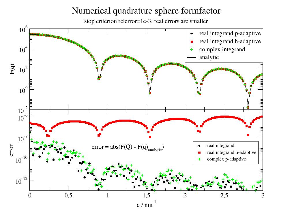
- jscatter.formel.pAC(func, lowlimit, uplimit, parnames, fdim=None, adaptive='p', abserr=1e-08, relerr=0.001, *args, **kwargs)
Vectorized adaptive multidimensional integration (cubature). Shortcut pAC.
We use the cubature module written by SG Johnson [2] for h-adaptive (recursively partitioning the integration domain into smaller subdomains) and p-adaptive (Clenshaw-Curtis quadrature, repeatedly doubling the degree of the quadrature rules). This function is a wrapper around the package cubature which can be used also directly.
- Parameters:
- funcfunction
The function to integrate. The return array needs to be an 2-dim array with the last dimension as vectorized return (=len(fdim)) and first along the points of the parnames parameters to integrate. Use numpy functions for array functions to speedup computations. See example.
- parnameslist of string
Parameter names of variables to integrate. Should be scalar.
- lowlimitlist of float
Lower limits of the integration variables with same length as parnames.
- uplimit: list of float
Upper limits of the integration variables with same length as parnames.
- fdimint, None, optional
Second dimension size of the func return array. If None, the function is evaluated with the uplimit values to determine the size. For complex valued function it is twice the complex array length.
- adaptive‘h’, ‘p’, default=’p’
Type of adaption algorithm.
‘h’ Multidimensional h-adaptive integration by subdividing the integration interval into smaller intervals where the same rule is applied.
The value and error in each interval is calculated from 7-point rule and difference to 5-point rule. For higher dimensions only the worst dimension is subdivided [3]. This algorithm is best suited for a moderate number of dimensions (say, < 7), and is superseded for high-dimensional integrals by other methods (e.g. Monte Carlo variants or sparse grids).
‘p’ Multidimensional p-adaptive integration by increasing the degree of the quadrature rule according to Clenshaw-Curtis quadrature
(in each iteration the number of points is doubled and the previous values are reused). Clenshaw-Curtis has similar error compared to Gaussian quadrature even if the used error estimate is worse. This algorithm is often superior to h-adaptive integration for smooth integrands in a few (≤ 3) dimensions,
- abserr, relerrfloat default = 1e-8, 1e-3
Absolute and relative error to stop. The integration will terminate when either the relative OR the absolute error tolerances are met. abserr=0, which means that it is ignored. The real error is much smaller than this stop criterion.
- maxEvalint, default 0, optional
Maximum number of function evaluations. 0 is infinite.
- normint, default=None, optional
Norm to evaluate the error.
None: 0,1 automatically choosen for real or complex functions.
0: individual for each integrand (real valued functions)
1: paired error (L2 distance) for complex values as distance in complex plane.
Other values as mentioned in cubature documentation.
- args,kwargsoptional
Additional arguments and keyword arguments passed to func.
- Returns:
- arrays values , error
Notes
The here used module jscatter.libs.cubature is an adaption of the Python interface of S.G.P. Castro [1] (vers. 0.14.5) to access the C-module of S.G. Johnson [2] (vers. 1.0.3). Only the vectorized form is realized here. The advantage here are fewer dependencies during install. Check the original packages for detailed documentation or look in jscatter.libs.cubature how to use it for your own things.
Internal: For complex valued functions the complex has to be split in real and imaginary to pass to the integration and later the result has to be converted to complex again. This is done automatically dependent on the return value of the function. For the example the real valued function is about 9 times faster
References
[3]An adaptive algorithm for numeric integration over an N-dimensional rectangular region A. C. Genz and A. A. Malik, J. Comput. Appl. Math. 6 (4), 295–302 (1980).
Examples
Integration of the sphere to get the sphere formfactor. In the first example the symmetry is used to return real valued amplitude. In the second the complex amplitude is used. Both can be compared to the analytic formfactor. Errors are much smaller than the abserr/relerr stop criterion. The stop seems to be related to the minimal point at q=2.8 as critical point. h-adaptive is for dim=3 less accurate and slower than p-adaptive.
The integrands contain patterns of scheme
q[:,None]*theta(with later .T to transpose, alternativeq*theta[:,None]) to result in a 2-dim array with the last dimension as vectorized return. The first dimension goes along the points to evaluate as determined from the algorithm.import jscatter as js import numpy as np R=5 q = np.r_[0.01:3:0.02] def sphere_real(r, theta, phi, b, q): res = b*np.cos(q[:,None]*r*np.cos(theta))*r**2*np.sin(theta)*2 return res.T pn = ['r','theta','phi'] fa_r,err = js.formel.pAC(sphere_real, [0,0,0], [R,np.pi/2,np.pi*2], pn, b=1, q=q) fa_rh,errh = js.formel.pAC(sphere_real, [0,0,0], [R,np.pi/2,np.pi*2], pn, b=1, q=q,adaptive='h') # As complex function def sphere_complex(r, theta, phi, b, q): fac = b * np.exp(1j * q[:, None] * r * np.cos(theta)) * r ** 2 * np.sin(theta) return fac.T fa_c, err = js.formel.pAC(sphere_complex, [0, 0, 0], [R, np.pi, np.pi * 2], pn, b=1, q=q) sp = js.ff.sphere(q, R) p = js.grace() p.multi(2,1,vgap=0) # integrals p[0].plot(q, fa_r ** 2, le='real integrand p-adaptive') p[0].plot(q, fa_rh ** 2, le='real integrand h-adaptive') p[0].plot(q, np.real(fa_c * np.conj(fa_c)),sy=[8,0.5,3], le='complex integrand') p[0].plot(q, sp.Y, li=1, sy=0, le='analytic') # errors p[1].plot(q,np.abs(fa_r**2 -sp.Y), le='real integrand') p[1].plot(q,np.abs(fa_rh**2 -sp.Y), le='real integrand h-adaptive') p[1].plot(q,np.abs(np.real(fa_c * np.conj(fa_c)) -sp.Y),sy=[8,0.5,3],le='complex p-adaptive') p[0].yaxis(scale='l',label='F(q)',ticklabel=['power',0]) p[0].xaxis(ticklabel=0) p[0].legend(x=2,y=1e6) p[1].legend(x=2.1,y=5e-9,charsize=0.8) p[1].yaxis(scale='l',label=r'error', ticklabel=['power',0],min=1e-13,max=5e-6) p[1].xaxis(label=r'q / nm\S-1') p[1].text(r'error = abs(F(Q) - F(q)\sanalytic\N)',x=0.8,y=1e-9,charsize=1) p[0].title('Numerical quadrature sphere formfactor ') p[0].subtitle('stop criterion relerror=1e-3, real errors are smaller') #p.save(js.examples.imagepath+'/cubature.jpg')
- jscatter.formel.Drot(Rh, Temp=293.15, solvent='h2o', visc=None)[source]
Rotational diffusion of a sphere.
\[D = \frac{k_\text{B} T}{8 \pi \eta R_h^3}\]- Parameters:
- Rhfloat
Hydrodynamic radius in nm.
- Tempfloat
Temperature in K.
- solventfloat
Solvent type as in viscosity; used if visc==None.
- viscfloat
Viscosity in Pas => H2O ~ 0.001 Pa*s =1 cPoise. If visc=None the solvent viscosity is calculated from function viscosity(solvent ,temp) with solvent e.g.’h2o’.
- Returns:
- float
Rotational diffusion coefficient in 1/ns.
- jscatter.formel.DrotfromT12(t12=None, Drot=None, F0=20000000.0, Tm=None, Ts=None, T1=None, T2=None)[source]
Rotational correlation time from T1/T2 or T1 and T2 from NMR proton relaxation measurement.
Allows to rescale by temperature and viscosity.
- Parameters:
- t12float
T1/T2 from NMR with unit seconds
- Drotfloat
!=None means output Drot instead of rotational correlation time.
- F0float
Resonance frequency of NMR instrument. For Hydrogen F0=20 MHz => w0=F0*2*np.pi
- Tm: float
Temperature of measurement in K.
- Tsfloat
Temperature needed for Drot -> rescaled by visc(T)/T.
- T1float
NMR T1 result in s
- T2float
NMR T2 result in s to calc t12 directly remeber if the sequence has a factor of 2
- Returns:
- float
Correlation time or Drot
Notes
See T1overT2
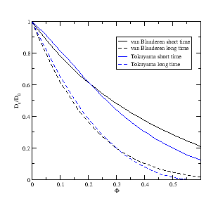
- jscatter.formel.DsoverDo(phi)[source]
\(D_s/D_0\) at short and long times for hard spheres with hydrodynamic and direct interctions.
The volume-fraction dependence of the short- and long-time self-diffusion coefficients.
- Parameters:
- phiarray
Volume fractions.
- Returns:
- Ds/D0dataArray
Columns ‘phi;bla_short;bla_long;toku_short;toku_long’ as
Access as result._bla_short or by index.
Notes
van Blaaderen et al [1] follows more the \(\delta\gamma\)-expansion of Beenakker & Mazur (see
hydrodynamicFunct()) :\[D_s^{short} = D_0 \frac{1 - \Phi}{1 + 3/2\Phi}\]\[D_s^{long} = D_0 \frac{(1 - \Phi)^3}{1 + 3/2 \Phi + 2\Phi^2 + 3 \Phi^3}\]Tokuyama & Oppenheim [2]
The formulation bears some similarity with that of Mazur [see ref 7 in [2]. The difference is that they start from the Navier-Stokes equation, while Mazur started from the quasistatic Stokes equation. :
\[\begin{split}D_s^{short} &= D_0/(1+L(\Phi)) \\ D_s^{long} &= \frac{D_0(1-9/32 \Phi) }{ (1 + L(\Phi) + K(\Phi)}\end{split}\]with
\[\begin{split}L(\Phi) &= \frac{2b^2}{(1-b)} - \frac{c}{(1+2c)} \\ &- \frac{2bc}{1-b+c} \left[1 - \frac{6bc}{1-b+c+4bc} + \frac{2bc}{1-b+c+2bc} \right] \\ &+ \frac{bc^2}{(1+c)(1-b+c)} \left[ 1+\frac{3bc^2}{(1+c)(1-b+c)-2bc^2} - \frac{bc^2}{(1+c)(1-b+c)-bc^2} \\ \right ]\end{split}\]\(b = (9\Phi/8)^{0.5}\) and \(c = 11\Phi/16\)
The first, second and third term result from long-range hydrodynamic interaction, short-range hydrodynamic interaction, and their coupling, respectively.
\(\Phi_0 = (4/3)^3 / (7ln(3)-8ln(2)+2)\) and
Nonlocal hydrodynamic effect \(K(\Phi) = \Phi/\Phi_0/(1-\Phi/\Phi_0)^2))\)
References
[1] (1,2,3)Long‐time self‐diffusion of spherical colloidal particles measured with fluorescence recovery after photobleaching. van Blaaderen, A., Peetermans, J., Maret, G., & Dhont, J. K. G. (1992). The Journal of Chemical Physics, 96(6), 4591–4603. https://doi.org/10.1063/1.462795
[2] (1,2,3,4)On the theory of concentrated hard-sphere suspensions. Tokuyama, M. & Oppenheim, I. Physica A: Statistical Mechanics and its Applications 216, 85–119 (1995).
[3]A simple formula for the short-time self-diffusion coefficient in concentrated suspensions P. Mazur, U. Geigenmüller Physica 146A (1987) 657-661, https://doi.org/10.1016/0378-4371(87)90291-3
Examples
import jscatter as js
import numpy as np

x=np.r_[0:0.6:30j]
ds = js.formel.DsoverDo(x)

p = js.grace(1.5,1.5)
p.plot(ds._phi,ds._bla_short,sy=0,li=[1,2,1],le='van Blaaderen short time')
p.plot(ds._phi,ds._bla_long,sy=0,li=[3,2,1],le='van Blaaderen long time')
p.plot(ds._phi,ds._toku_short,sy=0,li=[1,2,4],le='Tokuyama short time')
p.plot(ds._phi,ds._toku_long,sy=0,li=[3,2,4],le='Tokuyama long time')

p.yaxis(label=r'D\ss\N/D\s0',min=0,max=1)
p.xaxis(label=r'\xF',min=0,max=0.6)
p.legend(x=0.3,y=0.9)
# p.save(js.examples.imagepath+'/dsd0long.png',size=[1,1])
- jscatter.formel.Dtrans(Rh, Temp=293.15, solvent='h2o', visc=None)[source]
Translational diffusion of a sphere.
\[D = \frac{k_\text{B} T}{6 \pi \eta R_h}\]- Parameters:
- Rhfloat
Hydrodynamic radius in nm.
- Tempfloat
Temperature T in K.
- solventfloat
Solvent type as in viscosity; used if visc==None.
- viscfloat
Viscosity \(\eta\) in Pas => H2O ~ 0.001 Pas =1 cPoise. If visc=None the solvent viscosity is calculated from function viscosity(solvent ,temp) with solvent e.g.’h2o’ (see viscosity).
- Returns:
- Dfloat
Translational diffusion coefficient : float in nm^2/ns.
- jscatter.formel.Ea(z, a, b=1)[source]
Mittag-Leffler function for real z and real a,b with 0<a, b<0.
Evaluation of the Mittag-Leffler (ML) function with 1 or 2 parameters by means of the OPC algorithm [1]. The routine evaluates an approximation Et of the ML function E such that \(|E-Et|/(1+|E|) \approx 10^{-15}\)
- Parameters:
- zreal array
Values
- afloat, real positive
Parameter alpha
- bfloat, real positive, default=1
Parameter beta
- Returns:
- array
Notes
Mittag Leffler function defined as
\[E(x,a,b)=\sum_{k=0}^{\inf} \frac{z^k}{\Gamma(b+ak)}\]The code uses code from K.Hinsen at https://github.com/khinsen/mittag-leffler which is a Python port of Matlab implementation of the generalized Mittag-Leffler function as described in [1].
The function cannot be simply calculated by using the above summation. This fails for a,b<0.7 because of various numerical problems. The above implementation of K.Hinsen is the best availible approximation in Python.
References
[1]R. Garrappa, Numerical evaluation of two and three parameter Mittag-Leffler functions, SIAM Journal of Numerical Analysis, 2015, 53(3), 1350-1369
Examples
import numpy as np
import jscatter as js
from scipy import special
x=np.r_[-10:10:0.1]
# tests
np.all(js.formel.Ea(x,1,1)-np.exp(x)<1e-10)
z = np.linspace(0., 2., 50)
np.allclose(js.formel.Ea(np.sqrt(z), 0.5), np.exp(z)*special.erfc(-np.sqrt(z)))
z = np.linspace(-2., 2., 50)
np.allclose(js.formel.Ea(z**2, 2.), np.cosh(z))
- jscatter.formel.T1overT2(tr=None, Drot=None, F0=20000000.0, T1=None, T2=None)[source]
Calculates the T1/T2 from a given rotational correlation time tr or Drot for proton relaxation measurement.
tr=1/(6*D_rot) with rotational diffusion D_rot and correlation time tr.
- Parameters:
- trfloat
Rotational correlation time.
- Drotfloat
If given tr is calculated from Drot.
- F0float
NMR frequency e.g. F0=20e6 Hz=> w0=F0*2*np.pi is for Bruker Minispec with B0=0.47 Tesla
- T1float
NMR T1 result in s
- T2float
NMR T2 resilt in s to calc t12 directly
- Returns:
- float
T1/T2
Notes
\(J(\omega)=\tau/(1+\omega^2\tau^2)\)
\(T1^{-1}=\frac{\sigma}{3} (2J(\omega_0)+8J(2\omega_0))\)
\(T2^{-1}=\frac{\sigma}{3} (3J(0)+ 5J(\omega_0)+2J(2\omega_0))\)
\(tr=T1/T2\)
References
[1]Intermolecular electrostatic interactions and Brownian tumbling in protein solutions. Krushelnitsky A Physical chemistry chemical physics 8, 2117-28 (2006)
[2]The principle of nuclear magnetism A. Abragam Claredon Press, Oxford,1961
- jscatter.formel.aaVolume(aa)[source]
Volume of amino acids in A³ from Perkins [R0aa3310354ba-1] .
- Parameters:
- aastring
1 or 3 letter code
- Returns:
- list[consensus vol, error, 1 or 3 letter code, “Cohn_Edsall, Densitometry_1972, Densitometry_1984,
Molar_Group_Summations, Protein_Crystal_Structures, Amino_Acid_Crystal_Structures, ref number”]
References
- jscatter.formel.bicelleRh(Q, rim, thickness, k=1.6666666666666667)[source]
Hydrodynamic radius Rh of an ideal bicelle corrected for head group area.
- Parameters:
- Qfloat
Ratio of lipid composition
- rimfloat
Radius of the rim.
- thicknessfloat
Thickness of the bicelle planar region
- kfloat
Head group area ratio. like 1/0.6 for rim DHCP 1nm² and planar DMPC 0.6nm²
- Returns:
- [Rhfloat, R: float, R + rim] :
R radius of the planar region
Notes
Bicelle radius R with lipid area correction factor k [1] :
\[R = \frac{1}{2} k r Q [\pi +(\pi^2 + 8k/Q)^{1/2}]\]Rh of a (rectangular) disk with radius \(r^{\prime}\) and thickness t (same for a longer rod t>r’) [2] :
\[R_h = \frac{3}{2}r^{\prime} \Big[[1+(\frac{t}{2r^{\prime}})^2]^{1/2}-\frac{t}{2r^{\prime}} + \frac{2r^{\prime}}{t} ln\big(\frac{t}{2r^{\prime}} + [1+(\frac{t}{2r^{\prime}})^2]^{1/2}\big)\Big]^{-1}\]with \(r^{\prime} = R+r\) outer radius, rim radius \(r\), lipid ratio \(Q\), thickness t
It should be noted that in the references reporting this equation the hydrodynamic radius from DLS measurements is reported to be concentration dependent. This results from ignoring the structure factor effects (see
hydrodynamicFunct()) and leads to misinterpretation of the disc radius.References
[1]Structural Evaluation of Phospholipid Bicelles for Solution-State Studies of Membrane-Associated Biomolecules Glover, et al.Biophysical Journal 81(4), 2163–2171 (2001)
[2]Quasielastic Light-Scattering Studies of Aqueous Biliary Lipid Systems. Mixed Micelle Formation in Bile Salt-Lecithin Solutions Mazer et al.Biochemistry 19, 601–615 (1980), https://doi.org/10.1021/bi00545a001
- jscatter.formel.boseDistribution(w, temp)[source]
Bose distribution for integer spin particles in non-condensed state (hw>0).
\[ \begin{align}\begin{aligned}n(w) &= \frac{1}{e^{hw/kT}-1} &\ hw>0\\ &= 0 &\: hw=0 \: This is not real just for convenience!\end{aligned}\end{align} \]- Parameters:
- warray
Frequencies in units 1/ns
- tempfloat
Temperature in K
- Returns:
- dataArray
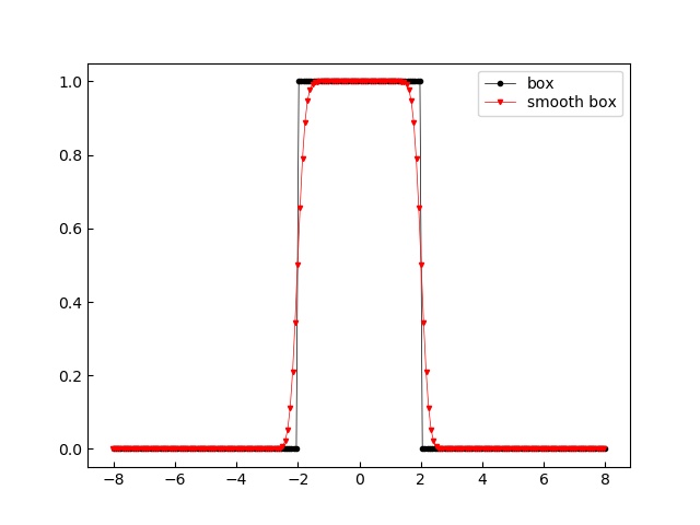
- jscatter.formel.box(x, edges=None, edgevalue=0, rtol=1e-05, atol=1e-08)[source]
Box function.
For equal edges and edge value > 0 the delta function is given.
- Parameters:
- xarray
- edgeslist of float, float, default=[0]
Edges of the box. If only one number is given the box goes from [-edge:edge]
- edgevaluefloat, default=0
Value to use if x==edge for both edges.
- rtol,atolfloat
The relative/absolute tolerance parameter for the edge detection. See numpy.isclose.
- Returns:
- dataArray
Notes
Edges may be smoothed by convolution with a Gaussian.:
import jscatter as js
import numpy as np
edge=2
x=np.r_[-4*edge:4*edge:200j]
f=js.formel.box(x,edges=edge)
res=js.formel.convolve(f,js.formel.gauss(x,0,0.2))
#
p=js.mplot()
p.Plot(f,li=1,le='box')
p.Plot(res,li=2,le='smooth box')
p.Legend()
#p.savefig(js.examples.imagepath+'/box.jpg')
- jscatter.formel.bufferviscosity(composition, T=293.15, show=False)[source]
Viscosity of water with inorganic substances as used in biological buffers.
Solvent with composition of H2O and D2O and additional components at temperature T. Ternary solutions allowed. Units are mol; 1l h2o = 55.50843 mol Based on data from ULTRASCAN3 [1] [2] supplemented by the viscosity of H2O/D2O mixtures for conc=0 [3] and [4].
- Parameters:
- compositionlist of compositional strings
Compositional strings of chemical name as ‘float’+’name’ First float is content in Mol followed by component name as ‘h2o’ or ‘d2o’ light and heavy water were mixed with prepended fractions.
[‘1.5urea’,’0.1sodiumchloride’,’2h2o’,’1d2o’] for 1.5 M urea + 100 mM NaCl in a 2:1 mixture of h2o/d2o. By default ‘1h2o’ is assumed.
- Tfloat, default 293.15
Temperature in K
- showbool, default False
Show composition and validity range of components and result in mPas.
- Returns:
- float
Viscosity in Pa*s
Notes
Viscosities of H2O/D2O mixtures mix by linear interpolation between concentrations (accuracy 0.2%) [3].
The change in viscosity due to components is added based on data from Ultrascan3 [1].
Multicomponent mixtures are composed of binary mixtures.
“Glycerol%” is in unit “%weight/weight” for range=”0-32%, here the unit is changed to weight% insthead of M.
Propanol1, Propanol2 are 1-Propanol, 2-Propanol
References
[2]Analytical Ultracentrifugation Data Analysis with UltraScan-III. Demeler, B.; Gorbet, G. E. In Analytical Ultracentrifugation: Instrumentation, Software, and Applications; Uchiyama, S., Arisaka, F., Stafford, W. F., Laue, T., Eds.; Springer Japan: Tokyo, 2016; pp 119–143. https://doi.org/10.1007/978-4-431-55985-6_8.
[3] (1,2)Viscosity of light and heavy water and their mixtures Kestin Imaishi Nott Nieuwoudt Sengers, Physica A: Statistical Mechanics and its Applications 134(1):38-58
[4]Thermal Offset Viscosities of Liquid H2O, D2O, and T2O C. H. Cho, J. Urquidi, S. Singh, and G. Wilse Robinson J. Phys. Chem. B 1999, 103, 1991-1994
availible components:
h2o1 d2o1
     aceticacid                acetone                   ammoniumacetate
 ammoniumchloride          ammoniumhydroxide         ammoniumsulfate
 bariumchloride            cadmiumchloride           cadmiumsulfate
 calciumchloride           cesiumchloride            citricacid
 cobaltouschloride         creatinine                cupricsulfate
 edtadisodium              ethanol                   ethyleneglycol
 ferricchloride            formicacid                fructose
 glucose                   glycerol                  glycerol%
 guanidinehydrochloride    hydrochloricacid          inulin
 lacticacid                lactose                   lanthanumnitrate
 leadnitrate               lithiumchloride           magnesiumchloride
 magnesiumsulfate          maltose                   manganoussulfate
 mannitol                  methanol                  nickelsulfate
 nitricacid                oxalicacid                phosphoricacid
 potassiumbicarbonate      potassiumbiphthalate      potassiumbromide
 potassiumcarbonate        potassiumchloride         potassiumchromate
 potassiumdichromate       potassiumferricyanide     potassiumferrocyanide
 potassiumhydroxide        potassiumiodide           potassiumnitrate
 potassiumoxalate          potassiumpermanganate     potassiumphosphate,dibasic
 potassiumphosphate,monobasic potassiumsulfate          potassiumthiocyanate
 procainehydrochloride     propanol1                 propanol2
 propyleneglycol           silvernitrate             sodiumacetate
 sodiumbicarbonate         sodiumbromide             sodiumcarbonate
 sodiumchloride            sodiumcitrate             sodiumdiatrizoate
 sodiumdichromate          sodiumferrocyanide        sodiumhydroxide
 sodiummolybdate           sodiumphosphate,dibasic   sodiumphosphate,monobasic
 sodiumphosphate,tribasic  sodiumsulfate             sodiumtartrate
 sodiumthiocyanate         sodiumthiosulfate         sodiumtungstate
 strontiumchloride         sucrose                   sulfuricacid
 tartaricacid              tetracainehydrochloride   trichloroaceticacid
 trifluoroethanol          tris                      tris(hydroxymethyl)aminomethane
 urea                      zincsulfate
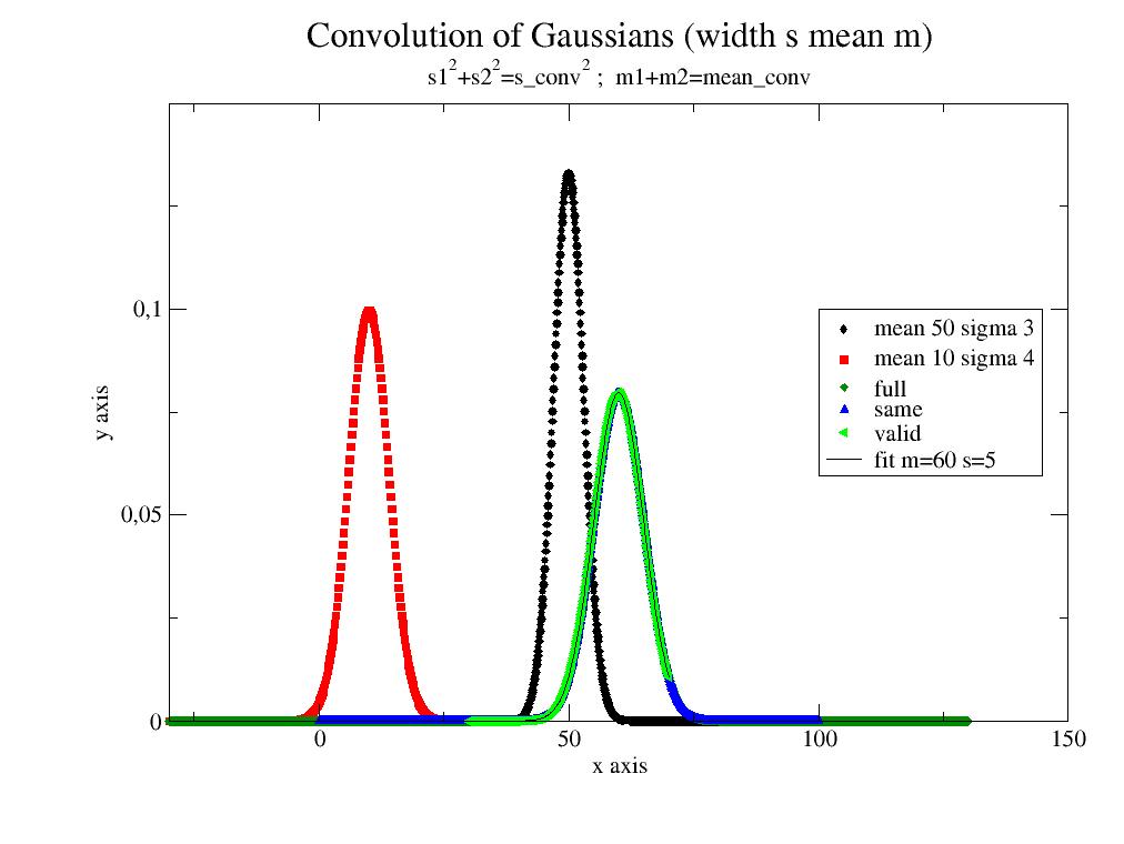
- jscatter.formel.convolve(A, B, mode='same', normA=False, normB=False)[source]
Convolve A and B with proper tracking of the output X axis mainly for inelastic scattering.
Approximate the convolution integral as the discrete, linear convolution of two one-dimensional sequences. Missing values are linear interpolated to have matching steps. Values outside of X ranges are set to zero.
- Parameters:
- A,BdataArray, ndarray
To be convolved arrays (length N and M).
dataArray convolves Y with Y values
ndarray A[0,:] is X and A[1,:] is Y
- normA,normBbool, default False
Determines if A or B should be normalized that \(\int_{x_{min}}^{x_{max}} A(x) dx = 1\).
- mode‘full’,’same’,’valid’, default ‘same’
See example for the difference in range.
‘full’ Returns the convolution at each point of overlap,
with an output shape of (N+M-1,). At the end-points of the convolution, the signals do not overlap completely, and boundary effects may be seen.
‘same’ Returns output of length max(M, N).
Boundary effects are still visible.
‘valid’ Returns output of length M-N+1.
For M==N or small differences the correct output may not what you expect.
- Returns:
- dataArray
with attributes from A
Notes
\(A\circledast B (t)= \int_{-\infty}^{\infty} A(x) B(t-x) dx = \int_{x_{min}}^{x_{max}} A(x) B(t-x) dx\)
If np.isclose(X,0) (zero in X values) then zero will be in the result. This is in particular for \(\delta\) distribution like in elastic_w(W) to make correct convolution with elastic term at zero.
If A,B are only 1d array use np.convolve.
If attributes of B are needed later use .setattr(B,’B-’) to prepend ‘B-’ for B attributes.
If A,B have non constant differences in X values the original X values can be recovered using interpolate
gg=js.formel.convolve(G1,G2,'same').interpolate(G1.X)References
[1]Wikipedia, “Convolution”, http://en.wikipedia.org/wiki/Convolution.
Examples
Demonstrate the difference between modes. Avoid ‘valid’ with equal length arrays because of singular values.
import jscatter as js;import numpy as np

s1=3;s2=4;m1=50;m2=10
G1=js.formel.gauss(np.r_[0:100.1:0.1],mean=m1,sigma=s1)
G2=js.formel.gauss(np.r_[-30:30.1:0.2],mean=m2,sigma=s2)

p=js.grace()
p.title('Convolution of Gaussians (width s mean m)')
p.subtitle(r's1\S2\N+s2\S2\N=s_conv\S2\N ;  m1+m2=mean_conv')
p.plot(G1,le='mean 50 sigma 3')
p.plot(G2,le='mean 10 sigma 4')

ggf=js.formel.convolve(G1,G2,'full')
p.plot(ggf,le='full')

ggs=js.formel.convolve(G1,G2,'same')
p.plot(ggs,le='same')

ggv=js.formel.convolve(G1,G2,'valid')
p.plot(ggv,le='valid')

ggv.fit(js.formel.gauss,{'mean':40,'sigma':1},{},{'x':'X'})
p.plot(ggv.modelValues(),li=1,sy=0,le='fit m=$mean s=$sigma')

p.legend(x=100,y=0.1)
p.xaxis(max=150,label='x axis')
p.yaxis(min=0,max=0.15,label='y axis')
p.save('convolve.jpg')
- jscatter.formel.cstar(Rg, Mw)[source]
Overlap concentration \(c^*\) for a polymer.
Equation 3 in [1] (Cotton) defines \(c^*\) as overlap concentration of space filling volumes corresponding to a cube or sphere with edge/radius equal to \(R_g\)
\[\frac{ M_w }{ N_A R_g^3} \approx c^* \approx \frac{3M_w}{4N_A \pi R_g^3}\]while equ. 4 uses cubes with \(2R_g\) (Graessley) \(c^* = \frac{ M_w }{ N_A 2R_g^3 }\) .
- Parameters:
- Rgfloat in nm
radius of gyration
- Mwfloat
molecular weight
- Returns:
- floatx3
Concentration limits [cube_rg, sphere_rg, cube_2rg] in units g/l.
References
[1]Overlap concentration of macromolecules in solution Ying, Q. & Chu, B. Macromolecules 20, 362–366 (1987)
- jscatter.formel.dielectricConstant(material='d2o', T=293.15, conc=0, delta=5.5)[source]
Dielectric constant of H2O and D2O buffer solutions.
Dielectric constant \(\epsilon\) of H2O and D2O (error +- 0.02) with added buffer salts.
\[\epsilon (c)=\epsilon (c=0)+2c\: delta\; for\; c<2M\]- Parameters:
- materialstring ‘d2o’ (default) or ‘h2o’
Material ‘d2o’ (default) or ‘h2o’
- Tfloat
Temperature in °C
- concfloat
Salt concentration in mol/l.
- deltafloat
Total excess polarisation dependent on the salt and presumably on the temperature!
- Returns:
- float
Dielectric constant
Notes
Salt
delta(+-1)
deltalambda (not used here)
HCl
-10
0
LiCl
7
-3.5
NaCl
5.5
- -4
default
KCl
5
-4
RbCl
5
-4.5
NaF
6
-4
KF
6.5
-3.5
NaI
-7.5
-9.5
KI
-8
-9.5
MgCI,
-15
-6
BaCl2
-14
-8.5
LaCI.
-22
-13.5
NaOH
-10.5
-3
Na2SO.
-11
-9.5
References
[1]Dielectric Constant of Water from 0 to 100 C. G . Malmberg and A. A. Maryott Journal of Research of the National Bureau of Standards, 56,1 ,369131-56–1 (1956) Research Paper 2641
[2]Dielectric Constant of Deuterium Oxide C.G Malmberg, Journal of Research of National Bureau of Standards, Vol 60 No 6, (1958) 2874 http://nvlpubs.nist.gov/nistpubs/jres/60/jresv60n6p609_A1b.pdf
[3]Dielectric Properties of Aqueous Ionic Solutions. Parts I and II Hasted et al. J Chem Phys 16 (1948) 1 http://link.aip.org/link/doi/10.1063/1.1746645
- jscatter.formel.doForList(funktion, looplist, *args, **kwargs)[source]
Parallel execution of a function in a pool of workers to speed up (multiprocessing).
Apply function with values in looplist in a pool of workers in parallel using multiprocessing. Like multiprocessing map_async but distributes automatically all given arguments.
- Parameters:
- funktionfunction
Function to process with arguments (args, loopover[i]=looplist[j,i], kwargs) Return value of function should contain parameters or at least the loopover value to allow a check, if desired.
- loopoverlist of string, default= None
Names of arguments to use for (sync) looping over with values in looplist.
If not given the first funktion argument is used.
If loopover is single argument this gets looplist[i,:]
Two arguments to loopover :
loopover=['q', 'iq']
- looplistlist or list of tuples with len(loopover)
List of values to loop over.
single argument just use a list
[0.01,0.1,0.2,0.3,0.4]for above ‘q’, ‘iq’ maybe
looplist=[(q, i) for i, q in enumerate([0.01,0.1,0.2,0.3,0.4])]
- ncpuint, optional
Number of cpus in the pool if started as main process (otherwise single process).
not given or 0 -> all cpus are used
int>0 min (ncpu, mp.cpu_count)
int<0 ncpu not to use
- cbNone, function
Callback after each calculation.
- debugint
debug > 0 allows serial output for testing.
- outputbool
If False no output is shown.
- Returns:
- listlist of function return values as [result1,result2,…..]
The order of return values is not explicitly synced to looplist. The return array may be prepended with the value looplist[i] as reference. E.g.:
def f(x,a,b,c,d):
result = x+a+b+c+d
    return [x, result]
Notes
Functions for parallel computations on a single multicore machine using the standard library multiprocessing.
Not the programming details, but the way how to speed up some things.
If your computation is already fast (e.g. <1s) go on without parallelisation. In an optimal case you gain a speedup as the number of cpu cores.
If you want to use a cluster with all cpus, this is not the way (you need MPI).
Parallelisation is no magic and this module is for convenience for non-specialist of parallel computing. The main thing is to pass additional parameters to the processes (a pool of workers) and loop only over one parameter given as list. Opening and closing of the pool is hidden in the function. In this way we can use a multicore machine with all cpus.
During testing, I found that shared memory does not really speed up in most cases, if we just want to calculate a function e.g. for a list of different Q values dependent on model parameters. Here the pickling of numpy arrays is efficient enough compared to the computation we do. The amount of data pickled should not be too large as each process gets a copy and pickling needs time.
If speed is an issue and shared memory gets important i advice using Fortran with OpenMP as used for ff.cloudScattering with parallel computation and shared memory. For me this was easier than the different solutions around.
We use here only non-modified input data and return a new dataset, so we don’t need to care about what happens if one process changes the data needed in another process (race conditions,…), anyway it’s not shared. Please keep this in mind and don’t complain if you find a way to modify input data.
For easier debugging (to find the position of an error in the pdb debugger) use the option debug. In this case the multiprocessing is not used and the debugger finds the error correctly.
Shared memory
Shared memory can be created and used with
shared_create(),shared_recover()andshared_close().See notes and example in
shared_create().Examples
Using in a module This is the prefered and intended way for usage that works on Linux, macOS and also on Windows.
Write a module like the following and name the file myfunctions.py .
import jscatter as js
import numpy as np

def f(x,a,b,c,d):
   res=x+a+b+c+d
   return [x,res]

def f2(x,a,b,c,d):
   res=x[0]+x[1]+a+b+c+d
   return [x[0],res]

def mycomplicatedModel(N,a,b,c,d):
    # using a list of 2 values for x (is first argument)
    loop = np.arange(N).reshape(-1,2)  # has 2 values in second dimension
    res = js.formel.doForList(f2,looplist=loop,a=a,b=b,c=c,d=d)
    return res
Create a working script where you use your functions defined in above module or do this on the command line.
import myfunctions as mf

res = mf.mycomplicatedModel(100,a=1,b=2,c=3,d=11)
Using in a simple script Not recommended! Already repeating is only possible with __spec__=None
This is what you find looking for multiprocessing in Windows as a typical usage pattern This is only neccessary on Windows but not on Linux or macOS
Take the following and paste it to script.py In a python shell do run scripy.py The calculation is encapsulated in the if clause and only executed on the main level. This if line is not needed for Linux or macOS
import jscatter as js
import numpy as np

def f(x,a,b,c,d):
   res=x+a+b+c+d
   return [x,res]

def f2(x,a,b,c,d):
   res=x[0]+x[1]+a+b+c+d
   return [x[0],res]

if __name__ == '__main__':
    __spec__ = None
    # loop over first argument, here x
    res = js.formel.doForList(f,looplist=np.arange(100),a=1,b=2,c=3,d=11)
    # loop over 'd' ignoring the given d=11 (which can be omitted here)
    res = js.formel.doForList(f,looplist=np.arange(100),loopover='d',x=0,a=1,b=2,c=3,d=11)

    # using a list of 2 values for x (is first argument)
    loop = np.arange(100).reshape(-1,2)  # has 2 values fin second dimension
    res = js.formel.doForList(f2,looplist=loop,a=1,b=2,c=3,d=11)

    # looping over several variables in sync
    loop = np.arange(100).reshape(-1,2)
    res = js.formel.doForList(f2,looplist=loop,loopover=['a','b'],x=[100,200],a=1,b=2,c=3,d=11)
- jscatter.formel.fibonacciLatticePointsOnSphere(NN, r=1)[source]
Fibonacci lattice points on a sphere with radius r (default r=1)
This can be used to integrate efficiently over a sphere with well distributed points.
- Parameters:
- NNinteger
number of points = 2*N+1
- rfloat, default 1
radius of sphere
- Returns:
- list of [r,phi,theta] pairs in radians
phi azimuth -pi<phi<pi; theta polar angle 0<theta<pi
References
[1]Measurement of Areas on a Sphere Using Fibonacci and Latitude–Longitude Lattices Á. González Mathematical Geosciences 42, 49-64 (2009)
Examples
import jscatter as js
import numpy as np
import matplotlib.pyplot as plt
from mpl_toolkits.mplot3d import Axes3D
points=js.formel.fibonacciLatticePointsOnSphere(1000)
pp=list(filter(lambda a:(a[1]>0) & (a[1]<np.pi/2) & (a[2]>0) & (a[2]<np.pi/2),points))
pxyz=js.formel.rphitheta2xyz(pp)
fig = plt.figure()
ax = fig.add_subplot(111, projection='3d')
ax.scatter(pxyz[:,0],pxyz[:,1],pxyz[:,2],color="k",s=20)
ax.set_xlim([-1,1])
ax.set_ylim([-1,1])
ax.set_zlim([-1,1])
plt.tight_layout()
plt.show(block=False)

points=js.formel.fibonacciLatticePointsOnSphere(1000)
pp=list(filter(lambda a:(a[2]>0.3) & (a[2]<1) ,points))
v=js.formel.rphitheta2xyz(pp)
R=js.formel.rotationMatrix([1,0,0],np.deg2rad(30))
pxyz=np.dot(R,v.T).T
#points in polar coordinates
prpt=js.formel.xyz2rphitheta(np.dot(R,pxyz.T).T)
fig = plt.figure()
ax = fig.add_subplot(111, projection='3d')
ax.scatter(pxyz[:,0],pxyz[:,1],pxyz[:,2],color="k",s=20)
ax.set_xlim([-1,1])
ax.set_ylim([-1,1])
ax.set_zlim([-1,1])
ax.set_xlabel('x')
ax.set_ylabel('y')
ax.set_zlabel('z')
plt.tight_layout()
plt.show(block=False)
- jscatter.formel.gauss(x, mean=1, sigma=1)[source]
Normalized Gaussian function.
\[g(x)= \frac{1}{sigma\sqrt{2\pi}} e^{-0.5(\frac{x-mean}{sigma})^2}\]- Parameters:
- xfloat
Values
- meanfloat
Mean value
- sigmafloat
1/e width. Negative values result in negative amplitude.
- Returns:
- dataArray
- jscatter.formel.haltonSequence(size, dim, skip=0)[source]
Pseudo random numbers from the Halton sequence in interval [0,1].
To use them as coordinate points transpose the array.
- Parameters:
- sizeint
Samples from the sequence
- dimint
Dimensions
- skipint
Number of points to skip in Halton sequence .
- Returns:
- array
Notes
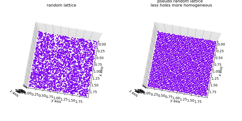
The visual difference between pseudorandom and random in 2D. See [2] for more details.
References
[1]https://mail.python.org/pipermail/scipy-user/2013-June/034741.html Author: Sebastien Paris, Josef Perktold translation from c
Examples
import jscatter as js
import numpy as np
import matplotlib.pyplot as plt
from mpl_toolkits.mplot3d import Axes3D
fig = plt.figure()
ax = fig.add_subplot(111, projection='3d')
for i,color in enumerate(['b','g','r','y']):
   # create halton sequence and shift it to needed shape
   pxyz=js.formel.haltonSequence(400,3).T*2-1
   ax.scatter(pxyz[:,0],pxyz[:,1],pxyz[:,2],color=color,s=20)
ax.set_xlim([-1,1])
ax.set_ylim([-1,1])
ax.set_zlim([-1,1])
plt.tight_layout()
plt.show(block=False)
- jscatter.formel.loglist(mini=0.1, maxi=5, number=100)[source]
Log like sequence between mini and maxi.
- Parameters:
- mini,maxifloat, default 0.1, 5
Start and endpoint.
- numberint, default 100
Number of points in sequence.
- Returns:
- ndarray
- jscatter.formel.lognorm(x, mean=1, sigma=1)[source]
Lognormal distribution function.
\[f(x>0)= \frac{1}{\sqrt{2\pi}\sigma x }\,e^{ -\frac{(\ln(x)-\mu)^2}{2\sigma^2}}\]- Parameters:
- xarray
x values
- meanfloat
mean
- sigmafloat
sigma
- Returns:
- dataArray
Examples
import numpy as np
import jscatter as js

x = np.r_[0:200:0.1]
fx = js.formel.lognorm(x,10,40)
mean = np.trapezoid(fx.Y*fx.X, fx.X)
sigma = np.trapezoid(fx.Y*(fx.X-10)**2, fx.X)
- jscatter.formel.lorentz(x, mean=1, gamma=1)[source]
Normalized Lorentz function
\[f(x) = \frac{gamma}{\pi((x-mean)^2+gamma^2)}\]- Parameters:
- xarray
X values
- gammafloat
Half width half maximum
- meanfloat
Mean value
- Returns:
- dataArray
- jscatter.formel.memoize(**memkwargs)[source]
A least-recently-used cache decorator to cache expensive function evaluations.
Memoize caches results and retrieves from cache if same parameters are used again. This can speedup computation in a model if a part is computed with same parameters several times. During fits it may be faster to calc result for a list and take from cache. See also https://docs.python.org/3/library/functools.html cache or lru_cache
The downside is that for large objects a lot of ram might be needed if a large amount of copies are cached.
- Parameters:
- functionfunction
Function to evaluate as e.g. f(Q,a,b,c,d)
- memkwargsdict
Keyword args with substitute values to cache for later interpolation. Empty for normal caching of a function. E.g. memkwargs={‘Q’:np.r_[0:10:0.1],’t’:np.r_[0:100:5]} caches with these values. The needed values can be interpolated from the returned result. See example below.
- maxsizeint, default 128
maximum size of the cache. Last is dropped.
- Returns:
- function
- cached function with new methods
last(i) to retrieve the ith evaluation result in cache (last is i=-1).
clear() to clear the cached results.
hitsmisses counts hits and misses.
Notes
Only keyword arguments for the memoized function are supported!!!! Only one attribute and X are supported for fitting as .interpolate works only for two cached attributes.
Examples
The example uses a model that computes like I(q,n,..)=F(q)*B(t,n,..). F(q) is cheap to calculate B(t,n,..) not. In the following its better to calc the function for a list of q , put it to cache and take in the fit from there. B is only calculated once inside of the function.
Use it like this:
import jscatter as js
import numpy as np

# define some data
TT=js.loglist(0.01,80,30)
QQ=np.r_[0.1:1.5:0.15]
# in the data we have 'q' and 'X'
data=js.dynamic.finiteZimm(t=TT,q=QQ,NN=124,pmax=100,tintern=10,l=0.38,Dcm=0.01,mu=0.5,viscosity=1.001,Temp=300)

# makes a unique list of all X values    -> interpolation is exact for X
# one may also use a smaller list of values and only interpolate
tt=list(set(data.X.flatten));tt.sort()

# define memoized function which will always use the here defined q and t
# use correct values from data for q     -> interpolation is exact for q
memfZ=js.formel.memoize(q=data.q,t=tt)(js.dynamic.finiteZimm)

def fitfunc(Q,Ti,NN,tint,ll,D,mu,viscosity,Temp):
   # use the memoized function as usual (even if given t and q are used from above definition)
   res= memfZ(NN=NN,tintern=tint,l=ll,Dcm=D,pmax=40,mu=mu,viscosity=viscosity,Temp=Temp)
   # interpolate to the here needed q and t (which is X)
   resint=res.interpolate(q=Q,X=Ti,deg=2)[0]
   return resint

# do the fit
data.setlimit(tint=[0.5,40],D=[0,1])
data.makeErrPlot(yscale='l')
NN=20
data.fit(model=fitfunc,
         freepar={'tint':10,'D':0.1,},
         fixpar={'NN':20,'ll':0.38/(NN/124.)**0.5,'mu':0.5,'viscosity':0.001,'Temp':300},
         mapNames={'Ti':'X','Q':'q'},)
Second example
Use memoize as a decorator (@ in front) acting on the following function. This is a shortcut for the above and works in the same way
# define the function to memoize
@js.formel.memoize(Q=np.r_[0:3:0.2],Time=np.r_[0:50:0.5,50:100:5])
def fZ(Q,Time,NN,tintern,ll,Dcm,mu,viscosity,Temp):
    # finiteZimm accepts t and q as array and returns a dataList with different Q and same X=t
    res=js.dynamic.finiteZimm(t=Time,q=Q,NN=NN,pmax=20,tintern=tintern,
                          l=ll,Dcm=Dcm,mu=mu,viscosity=viscosity,Temp=Temp)
    return res

# define the fitfunc
def fitfunc(Q,Ti,NN,tint,ll,D,mu,viscosity,Temp):
   #this is the cached result for the list of Q
   res= fZ(Time=Ti,Q=Q,NN=NN,tintern=tint,ll=ll,Dcm=D,mu=mu,viscosity=viscosity,Temp=Temp)
   # interpolate for the single Q value the cached result has again 'q'
   return res.interpolate(q=Q,X=Ti,deg=2)[0]

# do the fit
data.setlimit(tint=[0.5,40],D=[0,1])
data.makeErrPlot(yscale='l')
data.fit(model=fitfunc,
         freepar={'tint':6,'D':0.1,},
         fixpar={'NN':20,'ll':0.38/(20/124.)**0.5,'mu':0.5,'viscosity':0.001,'Temp':300},
         mapNames={'Ti':'X','Q':'q'})
# the result depends on the interpolation;
- jscatter.formel.molarity(objekt, c, total=None)[source]
Calculates the molarity.
- Parameters:
- objektobject,float
Objekt with method .mass() or molecular weight in Da.
- cfloat
Concentration in g/ml -> mass/Volume
- totalfloat, default None
Total volume in milliliter [ml] Concentration is calculated by c[g]/total[ml] if given.
- Returns:
- float
molarity in mol/liter (= mol/1000cm^3)
- jscatter.formel.multiParDistributedAverage(funktion, sigs, parnames, types='normal', N=30, ncpu=1, **kwargs)[source]
Vectorized average assuming multiple parameters are distributed in intervals. Shortcut mPDA.
Function average over multiple distributed parameters with weights determined from probability distribution. The probabilities for the parameters are multiplied as weights and a weighted sum is calculated by Monte-Carlo integration.
- Parameters:
- funktionfunction
Function to integrate with distribution weight.
- sigslist of float
List of widths for parameters. Sigs are the standard deviation from mean (or root of variance), see Notes.
- parnamesstring
List of names of the parameters which show a distribution.
- typeslist of ‘normal’, ‘lognorm’, ‘gamma’, ‘lorentz’, ‘uniform’, ‘poisson’, ‘schulz’, ‘duniform’, default ‘normal’
List of types of the distributions. If types list is shorter than parnames the last is repeated.
- kwargsparameters
Any additonal kword parameter to pass to function. The value of parnames that are distributed will be the mean value of the distribution.
- Nfloat , default=30
Number of points over distribution ranges. Distributions are integrated in probability intervals \([e^{-4} \ldots 1-e^{-4}]\).
- ncpuint, default=1, optional
Number of cpus in the pool for parallel excecution. Set this to 1 if the integrated function uses multiprocessing to avoid errors.
0 -> all cpus are used
int>0 min (ncpu, mp.cpu_count)
int<0 ncpu not to use
- Returns:
- dataArray
- as returned from function with
.parname_mean = mean of parname
.parname_std = standard deviation of parname
Notes
Calculation of an average over D multiple distributed parameters by conventional integration requires \(N^D\) function evaluations which is quite time consuming. Monte-Carlo integration at N points with random combinations of parameters requires only N evaluations.
The given function of fixed parameters \(q_j\) and polydisperse parameters \(p_i\) with width \(s_i\) related to the indicated distribution (types) is integrated as
\[f_{mean}(q_j,p_i,s_i) = \frac{\sum_h{f(q_j,x^h_i)\prod_i{w_i(x^h_i)}}}{\sum_h \prod_i w_i(x^h_i)}\]Each parameter \(p_i\) is distributed along values \(x^h_i\) with probability \(w_i(x^h_i)\) describing the probability distribution with mean \(p_i\) and sigma \(s_i\). Intervals for a parameter \(p_i\) are choosen to represent the distribution in the interval \([w_i(x^0_i) = e^{-4} \ldots \sum_h w_i(x^h_i) = 1-e^{-4}]\)
The distributed values \(x^h_i\) are determined as pseudorandom numbers of N points with dimension len(i) for Monte-Carlo integration.
For a single polydisperse parameter use parDistributedAverage.
During fitting it has to be accounted for the information content of the experimental data. As in the example below it might be better to use a single width for all parameters to reduce the number of redundant parameters.
The used distributions are from scipy.stats. Choose the distribution according to the problem and check needed number of points N.
mean is the value in kwargs[parname]. mean is the expectation value of the distributed variable and sig² are the variance as the expectation of the squared deviation from the mean. Distributions may be parametrized differently :
norm :
mean , stdstats.norm(loc=mean,scale=sig)lognorm :
mean and sig evaluate to mean and stdmu=math.log(mean**2/(sig+mean**2)**0.5)nu=(math.log(sig/mean**2+1))**0.5stats.lognorm(s=nu,scale=math.exp(mu))gamma :
mean and sig evaluate to mean and stdstats.gamma(a=mean**2/sig**2,scale=sig**2/mean)Same as SchulzZimmlorentz = cauchy:
mean and std are not defined. Use FWHM instead to describe width.sig=FWHMstats.cauchy(loc=mean,scale=sig))uniform :
Continuous distribution.sig is widthstats.uniform(loc=mean-sig/2.,scale=sig))poisson:
stats.poisson(mu=mean,loc=sig)
schulz
same as gammaduniform:
Uniform distribution integer values.sig>1stats.randint(low=mean-sig, high=mean+sig)
For more distribution look into this source code and use it appropriate with scipy.stats.
Examples
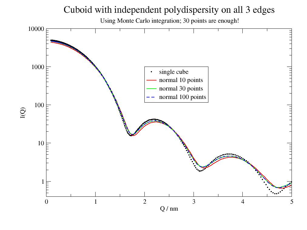
The example of a cuboid with independent polydispersity on all edges. To use the function in fitting please encapsulate it in a model function hiding the list parameters.
import jscatter as js
type=['norm','schulz']
p=js.grace()
q=js.loglist(0.1,5,500)
sp=js.ff.cuboid(q=q,a=4,b=4.1,c=4.3)
p.plot(sp,sy=[1,0.2],legend='single cube')
p.yaxis(scale='l',label='I(Q)')
p.xaxis(scale='n',label='Q / nm')

def cub(q,a,b,c):
   a = js.ff.cuboid(q=q,a=a,b=b,c=c)
   return a

p.title('Cuboid with independent polydispersity on all 3 edges')
p.subtitle('Using Monte Carlo integration; 30 points are enough here!')
sp1=js.formel.mPDA(cub,sigs=[0.2,0.3,0.1],parnames=['a','b','c'],types=type,q=q,a=4,b=4.1,c=4.2,N=10)
p.plot(sp1,li=[1,2,2],sy=0,legend='normal 10 points')
sp2=js.formel.mPDA(cub,sigs=[0.2,0.3,0.1],parnames=['a','b','c'],types=type,q=q,a=4,b=4.1,c=4.2,N=30)
p.plot(sp2,li=[1,2,3],sy=0,legend='normal 30 points')
sp3=js.formel.mPDA(cub,sigs=[0.2,0.3,0.1],parnames=['a','b','c'],types=type,q=q,a=4,b=4.1,c=4.2,N=90)
p.plot(sp3,li=[3,2,4],sy=0,legend='normal 100 points')
p.legend(x=2,y=1000)
# p.save(js.examples.imagepath+'/multiParDistributedAverage.jpg')
During fitting encapsulation might be done like this
def polyCube(a,b,c,sig,N):
   res = js.formel.mPDA(js.ff.cuboid,sigs=[sig,sig,sig],parnames=['a','b','c'],types='normal',q=q,a=a,b=b,c=c,N=N)
   return res
- jscatter.formel.pQACC(func, lowlimit, uplimit, parnames, weights0=None, weights1=None, weights2=None, rtol=1e-06, tol=1e-12, maxiter=520, miniter=8, **kwargs)
Vectorized adaptive multidimensional Clenshaw-Curtis quadrature for 1-3 dimensions. Shortcut pQACC.
Clenshaw-Curtis is superior to adaptive Gauss as for increased order the already calculated function values are reused. Convergence is similar to adaptive Gauss. In the cuboid example CC as fast as fixed GL with same number of points but GL is not adaptive.
- Parameters:
- funcfunction
A function or method to integrate. The return array needs to be a 2-dim array with the last dimension as vectorized return and first along the points of the parnames to integrate. Use numpy functions for array functions to speedup computations. See example.
- lowlimitlist of float
Lower limits of integration.
- uplimitlist of float
Upper limits of integration.
- parnameslist of strings
Names of the integration variables which should be scalar.
- weights0,weights1,weights2ndarray shape(2,N),default=None
Weights for integration along parname as a e.g. Gaussian distribution with a<weights[0]<b and weights[1] contains weight values.
Missing values are linear interpolated (faster).
If None equal weights=1 are used.
- kwargsdict, optional
Extra keyword arguments to pass to function, if any.
- tol, rtolfloat, optional
Iteration stops when (average) error between last two iterates is less than tol OR the relative change is less than rtol.
- maxiterint, default 520, optional
Maximum order of quadrature. Remember that the array of function values is of size iter**dim .
- miniterint, default 8, optional
Minimum order of quadrature.
- Returns:
- arrays values, error
Notes
Convergence of Clenshaw Curtis is about the same as Gauss-Legendre [1],[R1dc46e7e63c4-2]_.
Knots for evaluation include the borders -> [lowlimit,uplimit]. Check extremas there. Gauss-Legendre does not explicit the borders.
The iterative procedure reuses the previous calculated function values corresponding to F(n//2). Therefore eCC is faster
Error estimates are based on the difference between F(n) and F(n//2) which is on the order of other more sophisticated estimates [2].
Curse of dimension: The error for d-dim integrals is of order \(O(N^{-r/d})\) if the 1-dim integration method is \(O(N^{-r})\) with N as number of evaluation points in d-dim space. For Clenshaw-Curtis r is about 3 [2].
For higher dimensions used Monte-Carlo Methods (e.g. with pseudo random numbers).
References
[2] (1,2)Error estimation in the Clenshaw-Curtis quadrature formula H. O’Hara and Francis J. Smith The Computer Journal, 11, 213–219 (1968), https://doi.org/10.1093/comjnl/11.2.213
[3]Monte Carlo theory, methods and examples, chapter 7 Other quadrature methods Art B. Owen, 2019 https://artowen.su.domains/mc/Ch-quadrature.pdf
Examples
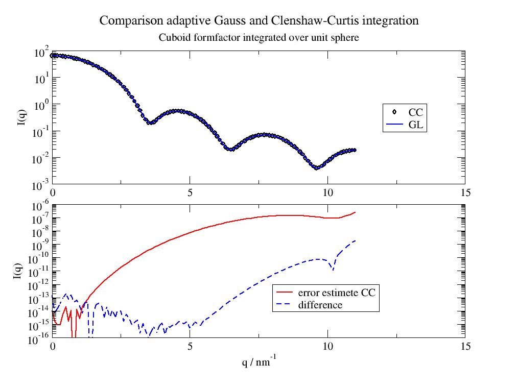
The cuboid formfactor includes an orientational average over the unit sphere which is done by integration over angles phi and theta which are our scalar integration variables. The array of q values are our vector input as we want to integrate for all q.
The integrand cuboid contains patterns of scheme
q*theta[:,None]to result in a 2-dim array with the last dimension as vectorized return. The first dimension goes along the points to evaluate as determined from the algorithm.For usage of weights see
parQuadratureFixedGaussxD()import jscatter as js import numpy as np pQACC = js.formel.pQACC # shortcut pQFGxD = js.formel.pQFGxD def cuboid(q, phi, theta, a, b, c): # integrand # scattering for orientations phi, theta as 1 dim arrays from 2dim integration # q is array for vectorized integration in last dimension # basically scheme as q*theta[:,None] results in array output of correct shape pi2 = np.pi * 2 fa = (np.sinc(q * a * np.sin(theta[:,None]) * np.cos(phi[:,None]) / pi2) * np.sinc(q * b * np.sin(theta[:,None]) * np.sin(phi[:,None]) / pi2) * np.sinc(q * c * np.cos(theta[:,None]) / pi2)) # add volume, sin(theta) weight of integration, normalise for unit sphere return fa**2*(a*b*c)**2*np.sin(theta[:,None])/np.pi/4 q=np.r_[0,0.1:11.1:0.1] NN=32 a,b,c = 2,2,2 # quadrature: use one quadrant and multiply later by 8 FqCC,err = pQACC(cuboid,[0,0],[np.pi/2,np.pi/2],parnames=['phi','theta'],q=q,a=a,b=b,c=c) FqCC8,err8 = pQACC(cuboid,[0,0],[np.pi/2,np.pi/2],parnames=['phi','theta'],q=q,a=a,b=b,c=c,rtol=1e-8) FqGL=js.formel.pQFGxD(cuboid,[0,0],[np.pi/2,np.pi/2],parnames=['phi','theta'],q=q,a=c,b=b,c=c,n=NN) p=js.grace() p.multi(2,1) p[0].title('Comparison adaptive Gauss and Clenshaw-Curtis integration',size=1.2) p[0].subtitle('Cuboid formfactor integrated over unit sphere') p[0].plot(q,FqCC*8,sy=1,le='CC rtol=1e-6') p[0].plot(q,FqCC8*8,sy=1,le='CC rtol=1e-8') p[0].plot(q,FqGL*8,sy=0,li=[1,2,4],le='GL') p[1].plot(q,err,li=[1,2,2],sy=0,le='error estimate CC rtol=1e-6') p[1].plot(q,err8,li=[1,2,2],sy=0,le='error estimate CC rtol=1e-8') p[1].plot(q,np.abs(FqCC*8-FqGL*8),li=[3,2,4],sy=0,le='|CC-GL|') p[0].xaxis(label=r'', min=0, max=15,) p[1].xaxis(label=r'q / nm\S-1', min=0, max=15) p[0].yaxis(label='I(q)',scale='log',ticklabel='power') p[1].yaxis(label='I(q)', scale='log',ticklabel='power', min=1e-16, max=1e-6) p[1].legend(y=1e-13,x=10,charsize=0.8) p[0].legend(y=1,x=12) #p.save(js.examples.imagepath+'/Clenshaw-Curtis.jpg')
- jscatter.formel.parAdaptiveCubature(func, lowlimit, uplimit, parnames, fdim=None, adaptive='p', abserr=1e-08, relerr=0.001, *args, **kwargs)[source]
Vectorized adaptive multidimensional integration (cubature). Shortcut pAC.
We use the cubature module written by SG Johnson [2] for h-adaptive (recursively partitioning the integration domain into smaller subdomains) and p-adaptive (Clenshaw-Curtis quadrature, repeatedly doubling the degree of the quadrature rules). This function is a wrapper around the package cubature which can be used also directly.
- Parameters:
- funcfunction
The function to integrate. The return array needs to be an 2-dim array with the last dimension as vectorized return (=len(fdim)) and first along the points of the parnames parameters to integrate. Use numpy functions for array functions to speedup computations. See example.
- parnameslist of string
Parameter names of variables to integrate. Should be scalar.
- lowlimitlist of float
Lower limits of the integration variables with same length as parnames.
- uplimit: list of float
Upper limits of the integration variables with same length as parnames.
- fdimint, None, optional
Second dimension size of the func return array. If None, the function is evaluated with the uplimit values to determine the size. For complex valued function it is twice the complex array length.
- adaptive‘h’, ‘p’, default=’p’
Type of adaption algorithm.
‘h’ Multidimensional h-adaptive integration by subdividing the integration interval into smaller intervals where the same rule is applied.
The value and error in each interval is calculated from 7-point rule and difference to 5-point rule. For higher dimensions only the worst dimension is subdivided [3]. This algorithm is best suited for a moderate number of dimensions (say, < 7), and is superseded for high-dimensional integrals by other methods (e.g. Monte Carlo variants or sparse grids).
‘p’ Multidimensional p-adaptive integration by increasing the degree of the quadrature rule according to Clenshaw-Curtis quadrature
(in each iteration the number of points is doubled and the previous values are reused). Clenshaw-Curtis has similar error compared to Gaussian quadrature even if the used error estimate is worse. This algorithm is often superior to h-adaptive integration for smooth integrands in a few (≤ 3) dimensions,
- abserr, relerrfloat default = 1e-8, 1e-3
Absolute and relative error to stop. The integration will terminate when either the relative OR the absolute error tolerances are met. abserr=0, which means that it is ignored. The real error is much smaller than this stop criterion.
- maxEvalint, default 0, optional
Maximum number of function evaluations. 0 is infinite.
- normint, default=None, optional
Norm to evaluate the error.
None: 0,1 automatically choosen for real or complex functions.
0: individual for each integrand (real valued functions)
1: paired error (L2 distance) for complex values as distance in complex plane.
Other values as mentioned in cubature documentation.
- args,kwargsoptional
Additional arguments and keyword arguments passed to func.
- Returns:
- arrays values , error
Notes
The here used module jscatter.libs.cubature is an adaption of the Python interface of S.G.P. Castro [1] (vers. 0.14.5) to access the C-module of S.G. Johnson [2] (vers. 1.0.3). Only the vectorized form is realized here. The advantage here are fewer dependencies during install. Check the original packages for detailed documentation or look in jscatter.libs.cubature how to use it for your own things.
Internal: For complex valued functions the complex has to be split in real and imaginary to pass to the integration and later the result has to be converted to complex again. This is done automatically dependent on the return value of the function. For the example the real valued function is about 9 times faster
References
[3]An adaptive algorithm for numeric integration over an N-dimensional rectangular region A. C. Genz and A. A. Malik, J. Comput. Appl. Math. 6 (4), 295–302 (1980).
Examples
Integration of the sphere to get the sphere formfactor. In the first example the symmetry is used to return real valued amplitude. In the second the complex amplitude is used. Both can be compared to the analytic formfactor. Errors are much smaller than the abserr/relerr stop criterion. The stop seems to be related to the minimal point at q=2.8 as critical point. h-adaptive is for dim=3 less accurate and slower than p-adaptive.
The integrands contain patterns of scheme
q[:,None]*theta(with later .T to transpose, alternativeq*theta[:,None]) to result in a 2-dim array with the last dimension as vectorized return. The first dimension goes along the points to evaluate as determined from the algorithm.import jscatter as js import numpy as np R=5 q = np.r_[0.01:3:0.02] def sphere_real(r, theta, phi, b, q): res = b*np.cos(q[:,None]*r*np.cos(theta))*r**2*np.sin(theta)*2 return res.T pn = ['r','theta','phi'] fa_r,err = js.formel.pAC(sphere_real, [0,0,0], [R,np.pi/2,np.pi*2], pn, b=1, q=q) fa_rh,errh = js.formel.pAC(sphere_real, [0,0,0], [R,np.pi/2,np.pi*2], pn, b=1, q=q,adaptive='h') # As complex function def sphere_complex(r, theta, phi, b, q): fac = b * np.exp(1j * q[:, None] * r * np.cos(theta)) * r ** 2 * np.sin(theta) return fac.T fa_c, err = js.formel.pAC(sphere_complex, [0, 0, 0], [R, np.pi, np.pi * 2], pn, b=1, q=q) sp = js.ff.sphere(q, R) p = js.grace() p.multi(2,1,vgap=0) # integrals p[0].plot(q, fa_r ** 2, le='real integrand p-adaptive') p[0].plot(q, fa_rh ** 2, le='real integrand h-adaptive') p[0].plot(q, np.real(fa_c * np.conj(fa_c)),sy=[8,0.5,3], le='complex integrand') p[0].plot(q, sp.Y, li=1, sy=0, le='analytic') # errors p[1].plot(q,np.abs(fa_r**2 -sp.Y), le='real integrand') p[1].plot(q,np.abs(fa_rh**2 -sp.Y), le='real integrand h-adaptive') p[1].plot(q,np.abs(np.real(fa_c * np.conj(fa_c)) -sp.Y),sy=[8,0.5,3],le='complex p-adaptive') p[0].yaxis(scale='l',label='F(q)',ticklabel=['power',0]) p[0].xaxis(ticklabel=0) p[0].legend(x=2,y=1e6) p[1].legend(x=2.1,y=5e-9,charsize=0.8) p[1].yaxis(scale='l',label=r'error', ticklabel=['power',0],min=1e-13,max=5e-6) p[1].xaxis(label=r'q / nm\S-1') p[1].text(r'error = abs(F(Q) - F(q)\sanalytic\N)',x=0.8,y=1e-9,charsize=1) p[0].title('Numerical quadrature sphere formfactor ') p[0].subtitle('stop criterion relerror=1e-3, real errors are smaller') #p.save(js.examples.imagepath+'/cubature.jpg')
- jscatter.formel.parDistributedAverage(funktion, sig, parname, type='norm', nGauss=30, **kwargs)[source]
Vectorized average assuming a single parameter is distributed with width sig. Shortcut pDA.
Function average over a parameter with weights determined from probability distribution. Gaussian quadrature over given distribution or summation with weights is used. All columns are integrated except .X for dataArray.
- Parameters:
- funktionfunction
Function to integrate with distribution weight. Function needs to return dataArray. All columns except .X are integrated.
- sigfloat
Standard deviation from mean (root of variance) or location describing the width the distribution, see Notes.
- parnamestring
Name of the parameter of funktion which shows a distribution.
- type‘normal’,’lognorm’,’gamma’,’lorentz’,’uniform’,’poisson’,’schulz’,’duniform’,’truncnorm’ default ‘norm’
Type of the distribution
- kwargsparameters
Any additional keyword parameter to pass to function or distribution. The value of parname will be the mean value of the distribution.
- nGaussfloat , default=30
Order of quadrature integration as number of intervals in Gauss–Legendre quadrature over distribution. Distribution is integrated in probability interval [0.001..0.999].
- ncpuint, optional
Number of cpus in the pool. Set this to 1 if the integrated function uses multiprocessing to avoid errors.
0 -> all cpus are used
int>0 min (ncpu, mp.cpu_count)
int<0 ncpu not to use
- Returns:
- outdataArray
as returned from function with
.parname_mean : mean of parname
.parname_std : standard deviation of parname (root of variance, input parameter)
.pdf : probability distribution within some range.
Notes
The used distributions are from scipy.stats. Choose the distribution according to the problem.
mean is the value in kwargs[parname]. mean is the expectation value of the distributed variable.
sig² is the variance as the expectation of the squared deviation from the mean.
Distributions may be parametrized differently with additional parameters :
norm :
mean , sigstats.norm(loc=mean,scale=sig)here sig scales the positiontruncnorm
mean , sig; a,b lower and upper cutoffsa,b are in scale of sig around mean;absolute cutoff c,d change to a, b = (c-mean)/sig, (d-mean)/sigstats.norm(a,b,loc=mean,scale=sig)lognorm :
mean and sig evaluate to (see https://en.wikipedia.org/wiki/Log-normal_distribution)a = 1 + (sig / mean) ** 2s = np.sqrt(np.log(a))scale = mean / np.sqrt(a)stats.lognorm(s=s,scale=scale)gamma :
mean and sigstats.gamma(a=mean**2/sig**2,scale=sig**2/mean)Same as SchulzZimmlorentz = cauchy :
mean and sig are not defined. Use FWHM instead to describe width.sig=FWHMstats.cauchy(loc=mean,scale=sig))uniform :
Continuous distribution.sig is widthstats.uniform(loc=mean-sig/2.,scale=sig))schulz
Same as gammapoisson:
stats.poisson(mu=mean,loc=sig)
duniform:
Uniform distribution integer values.sig>1stats.randint(low=mean-sig, high=mean+sig)
For more distribution look into this source code and use it appropriate with scipy.stats.
Examples
import jscatter as js
p=js.grace()
q=js.loglist(0.1,5,500)
sp=js.ff.sphere(q=q,radius=5)
p.plot(sp,sy=[1,0.2],legend='single radius')
p.yaxis(scale='l',label='I(Q)')
p.xaxis(scale='n',label='Q / nm')
sig=0.2
p.title('radius distribution with width %.g' %(sig))

sp2=js.formel.pDA(js.ff.sphere,sig,'radius',type='norm',q=q,radius=5,nGauss=100)
p.plot(sp2,li=[1,2,2],sy=0,legend='normal 100 points Gauss ')

sp4=js.formel.pDA(js.ff.sphere,sig,'radius',type='normal',q=q,radius=5,nGauss=30)
p.plot(sp4,li=[1,2,3],sy=0,legend='normal 30 points Gauss  ')

sp5=js.formel.pDA(js.ff.sphere,sig,'radius',type='normal',q=q,radius=5,nGauss=5)
p.plot(sp5,li=[1,2,5],sy=0,legend='normal 5 points Gauss  ')

sp3=js.formel.pDA(js.ff.sphere,sig,'radius',type='lognorm',q=q,radius=5)
p.plot(sp3,li=[3,2,4],sy=0,legend='lognorm')

sp6=js.formel.pDA(js.ff.sphere,sig,'radius',type='gamma',q=q,radius=5)
p.plot(sp6,li=[2,2,6],sy=0,legend='gamma ')

sp9=js.formel.pDA(js.ff.sphere,sig,'radius',type='schulz',q=q,radius=5)
p.plot(sp9,li=[3,2,2],sy=0,legend='SchulzZimm ')

# an unrealistic example
sp7=js.formel.pDA(js.ff.sphere,1,'radius',type='poisson',q=q,radius=5)
p.plot(sp7,li=[1,2,6],sy=0,legend='poisson ')

sp8=js.formel.pDA(js.ff.sphere,1,'radius',type='duniform',q=q,radius=5)
p.plot(sp8,li=[1,2,6],sy=0,legend='duniform ')
p.legend()
- jscatter.formel.parQuadratureAdaptiveClenshawCurtis(func, lowlimit, uplimit, parnames, weights0=None, weights1=None, weights2=None, rtol=1e-06, tol=1e-12, maxiter=520, miniter=8, **kwargs)[source]
Vectorized adaptive multidimensional Clenshaw-Curtis quadrature for 1-3 dimensions. Shortcut pQACC.
Clenshaw-Curtis is superior to adaptive Gauss as for increased order the already calculated function values are reused. Convergence is similar to adaptive Gauss. In the cuboid example CC as fast as fixed GL with same number of points but GL is not adaptive.
- Parameters:
- funcfunction
A function or method to integrate. The return array needs to be a 2-dim array with the last dimension as vectorized return and first along the points of the parnames to integrate. Use numpy functions for array functions to speedup computations. See example.
- lowlimitlist of float
Lower limits of integration.
- uplimitlist of float
Upper limits of integration.
- parnameslist of strings
Names of the integration variables which should be scalar.
- weights0,weights1,weights2ndarray shape(2,N),default=None
Weights for integration along parname as a e.g. Gaussian distribution with a<weights[0]<b and weights[1] contains weight values.
Missing values are linear interpolated (faster).
If None equal weights=1 are used.
- kwargsdict, optional
Extra keyword arguments to pass to function, if any.
- tol, rtolfloat, optional
Iteration stops when (average) error between last two iterates is less than tol OR the relative change is less than rtol.
- maxiterint, default 520, optional
Maximum order of quadrature. Remember that the array of function values is of size iter**dim .
- miniterint, default 8, optional
Minimum order of quadrature.
- Returns:
- arrays values, error
Notes
Convergence of Clenshaw Curtis is about the same as Gauss-Legendre [1],[R9195a8e64944-2]_.
Knots for evaluation include the borders -> [lowlimit,uplimit]. Check extremas there. Gauss-Legendre does not explicit the borders.
The iterative procedure reuses the previous calculated function values corresponding to F(n//2). Therefore eCC is faster
Error estimates are based on the difference between F(n) and F(n//2) which is on the order of other more sophisticated estimates [2].
Curse of dimension: The error for d-dim integrals is of order \(O(N^{-r/d})\) if the 1-dim integration method is \(O(N^{-r})\) with N as number of evaluation points in d-dim space. For Clenshaw-Curtis r is about 3 [2].
For higher dimensions used Monte-Carlo Methods (e.g. with pseudo random numbers).
References
[2] (1,2)Error estimation in the Clenshaw-Curtis quadrature formula H. O’Hara and Francis J. Smith The Computer Journal, 11, 213–219 (1968), https://doi.org/10.1093/comjnl/11.2.213
[3]Monte Carlo theory, methods and examples, chapter 7 Other quadrature methods Art B. Owen, 2019 https://artowen.su.domains/mc/Ch-quadrature.pdf
Examples
The cuboid formfactor includes an orientational average over the unit sphere which is done by integration over angles phi and theta which are our scalar integration variables. The array of q values are our vector input as we want to integrate for all q.
The integrand cuboid contains patterns of scheme
q*theta[:,None]to result in a 2-dim array with the last dimension as vectorized return. The first dimension goes along the points to evaluate as determined from the algorithm.For usage of weights see
parQuadratureFixedGaussxD()import jscatter as js import numpy as np pQACC = js.formel.pQACC # shortcut pQFGxD = js.formel.pQFGxD def cuboid(q, phi, theta, a, b, c): # integrand # scattering for orientations phi, theta as 1 dim arrays from 2dim integration # q is array for vectorized integration in last dimension # basically scheme as q*theta[:,None] results in array output of correct shape pi2 = np.pi * 2 fa = (np.sinc(q * a * np.sin(theta[:,None]) * np.cos(phi[:,None]) / pi2) * np.sinc(q * b * np.sin(theta[:,None]) * np.sin(phi[:,None]) / pi2) * np.sinc(q * c * np.cos(theta[:,None]) / pi2)) # add volume, sin(theta) weight of integration, normalise for unit sphere return fa**2*(a*b*c)**2*np.sin(theta[:,None])/np.pi/4 q=np.r_[0,0.1:11.1:0.1] NN=32 a,b,c = 2,2,2 # quadrature: use one quadrant and multiply later by 8 FqCC,err = pQACC(cuboid,[0,0],[np.pi/2,np.pi/2],parnames=['phi','theta'],q=q,a=a,b=b,c=c) FqCC8,err8 = pQACC(cuboid,[0,0],[np.pi/2,np.pi/2],parnames=['phi','theta'],q=q,a=a,b=b,c=c,rtol=1e-8) FqGL=js.formel.pQFGxD(cuboid,[0,0],[np.pi/2,np.pi/2],parnames=['phi','theta'],q=q,a=c,b=b,c=c,n=NN) p=js.grace() p.multi(2,1) p[0].title('Comparison adaptive Gauss and Clenshaw-Curtis integration',size=1.2) p[0].subtitle('Cuboid formfactor integrated over unit sphere') p[0].plot(q,FqCC*8,sy=1,le='CC rtol=1e-6') p[0].plot(q,FqCC8*8,sy=1,le='CC rtol=1e-8') p[0].plot(q,FqGL*8,sy=0,li=[1,2,4],le='GL') p[1].plot(q,err,li=[1,2,2],sy=0,le='error estimate CC rtol=1e-6') p[1].plot(q,err8,li=[1,2,2],sy=0,le='error estimate CC rtol=1e-8') p[1].plot(q,np.abs(FqCC*8-FqGL*8),li=[3,2,4],sy=0,le='|CC-GL|') p[0].xaxis(label=r'', min=0, max=15,) p[1].xaxis(label=r'q / nm\S-1', min=0, max=15) p[0].yaxis(label='I(q)',scale='log',ticklabel='power') p[1].yaxis(label='I(q)', scale='log',ticklabel='power', min=1e-16, max=1e-6) p[1].legend(y=1e-13,x=10,charsize=0.8) p[0].legend(y=1,x=12) #p.save(js.examples.imagepath+'/Clenshaw-Curtis.jpg')
- jscatter.formel.parQuadratureAdaptiveGauss(func, lowlimit, uplimit, parname, weights=None, tol=1e-08, rtol=1e-08, maxiter=150, miniter=8, **kwargs)[source]
Vectorized definite integral using fixed-tolerance Gaussian quadrature. Shortcut pQAG.
parQuadratureAdaptiveClenshawCurtis is more efficient but includes border values explicit.
Adaptive integration of func from a to b using Gaussian quadrature adaptivly increasing number of points by 8. All columns are integrated. For func return values as dataArray the .X is recovered (unscaled) while for array also the X are integrated and weighted.
- Parameters:
- funcfunction
A function or method to integrate returning an array or dataArray.
- lowlimitfloat
Lower limit of integration.
- uplimitfloat
Upper limit of integration.
- parnamestring
name of the integration variable which should be a scalar.
- weightsndarray shape(2,N),default=None
Weights for integration along parname as a Gaussian with lowlimit<weights[0]<uplimit and weights[1] contains weight values.
Missing values are linear interpolated (faster).
If None equal weights=1 are used.
- kwargsdict, optional
Extra keyword arguments to pass to function, if any.
- tol, rtolfloat, optional
Iteration stops when error between last two iterates is less than tol OR the relative change is less than rtol.
- maxiterint, default 150, optional
Maximum order of Gaussian quadrature.
- miniterint, default 8, optional
Minimum order of Gaussian quadrature.
- ncpuint, default=1, optional
Number of cpus in the pool. Set this to 1 if the integrated function uses multiprocessing to avoid errors.
0 -> all cpus are used
int>0 min (ncpu, mp.cpu_count)
int<0 ncpu not to use
- Returns:
- valfloat
Gaussian quadrature approximation (within tolerance) to integral for all vector elements.
- errfloat
Difference between last two estimates of the integral.
Notes
Reimplementation of scipy.integrate.quadrature.quadrature to work with vector output of the integrand function.
References
Examples
A simple polydispersity: integrate size distribution of equal weight. Normalisation by 4sig.
We see that Rg and I0 at low Q also change because of polydispersity. Minima are smeared out.
import jscatter as js
q=js.loglist(0.01,5,500)
p=js.grace()
mean=5
for sig in [0.01,0.1,0.3,0.4]:  # distribution width
    sp2=js.formel.pQAG(js.ff.sphere,mean-2*sig,mean+2*sig,'radius',q=q,radius=mean)
    p.plot(sp2.X, sp2.Y/(4*sig),sy=[-1,0.2,-1])
p.yaxis(scale='l')
Integrate Gaussian as test case. As we integrate over .X the final .X will be the first integration point .X, here the first Legendre knot.
t=np.r_[1:100]
gg=js.formel.gauss(t,50,10)
js.formel.pQAG(js.formel.gauss,0,100,'x',mean=50,sigma=10)
- jscatter.formel.parQuadratureFixedGauss(func, lowlimit, uplimit, parname, n=25, weights=None, **kwargs)[source]
Vectorized definite integral using fixed-order Gaussian quadrature. Shortcut pQFG.
Integrate func over parname from lowlimit to uplimit using Gauss-Legendre quadrature [1] of order n. All columns are integrated. For func return values as dataArray the .X is recovered (unscaled) while for array also the X are integrated and weighted.
- Parameters:
- funccallable
A Python function or method returning a vector array of dimension 1. If func returns dataArray .Y is integrated.
- lowlimitfloat
Lower limit of integration.
- uplimitfloat
Upper limit of integration.
- parnamestring
Name of the integration variable which should be a scalar. After evaluation the corresponding attribute has the mean value with weights.
- weightsndarray shape(2,N),default=None
Weights for integration along parname with lowlimit<weights[0]<uplimit and weights[1] as weight values.
Missing values are linear interpolated.
If None equal weights=1 are used. To use normalized weights normalise it or use scipy.stats distributions.
- kwargsdict, optional
Extra keyword arguments to pass to function, if any.
- nint, optional
Order of quadrature integration. Default is 15.
- ncpuint,default=1, optional
Use parallel processing for the function with ncpu parallel processes in the pool. Set this to 1 if the function is already fast enough or if the integrated function uses multiprocessing.
0 -> all cpus are used
int>0 min (ncpu, mp.cpu_count)
int<0 ncpu not to use
- Returns:
- array or dataArray
Notes
Gauss-Legendre quadrature of function \(f(x,p)\) over parameter \(p\) with a weight function \(v(p)\)
Reimplementation of scipy.integrate.quadrature.fixed_quad to work with vector output of the integrand function and weights.
\(w_i\) and \(p_i\) are the associated weights and knots of the Legendre polynominals.
\[\int_{-1}^1 f(x,p) v(p) dp \approx \sum_{i=1}^n w_i v_i f(x,p_i)\]Change of interval to [a,b] is done as
\[\int_a^b f(x, p)\,dp = \int_{-1}^1 \left(\frac{b-a}{2}\xi + \frac{a+b}{2}\right) \frac{dx}{d\xi}d\xi\]with \(\frac{dx}{d\xi} = \frac{b-a}{2}\) .
Knots for evaluation do NOT include the borders explicitly -> ]lowlimit,uplimit[.
References
Examples
A simple polydispersity of spheres: integrate size distribution with weights.
We see that Rg and I0 at low Q also change because of polydispersity. \(I_0~R^6\). Minima are smeared out.
For a Gaussian distribution the edge values are less weighted but broader and the central values are stronger weighted. The effect on I0 is stronger and the minima are more smeared.
The uniform distribution is the same as weights=None, but normalized to 1. Using None we get the same (weight=1) if the result is normalized by the width 2*sig.
import jscatter as js
import numpy as np
import scipy
q=js.loglist(0.01,5,500)
p=js.grace()
p.multi(2,1)
mean=5

# use a uniform distribution
for sig in [0.1,0.5,0.8,1]:  # distribution width
    distrib = scipy.stats.uniform(loc=mean-sig,scale=2*sig)
    x = np.r_[mean-3*sig:mean+3*sig:30j]
    pdf = np.c_[x,distrib.pdf(x)].T
    sp2 = js.formel.pQFG(js.ff.sphere,mean-sig,mean+sig,'radius',q=q,radius=mean,n=20, weights=pdf)
    p[0].plot(sp2.X, sp2.Y,sy=[-1,0.2,-1])
p[0].yaxis(label='I(Q)',scale='l')
p[0].xaxis(label=r'')
p[0].text('uniform distribution',x=2,y=1e5)

# use a Gaussian distribution
for sig in [0.1,0.5,0.8,1]:  # distribution width
    distrib = scipy.stats.norm(loc=mean,scale=sig)
    x = np.r_[mean-3*sig:mean+3*sig:30j]
    pdf = np.c_[x,distrib.pdf(x)].T
    sp2 = js.formel.pQFG(js.ff.sphere,mean-2*sig,mean+2*sig,'radius',q=q,radius=mean,n=25,weights=pdf)
    p[1].plot(sp2.X, sp2.Y,sy=[-1,0.2,-1])
p[1].yaxis(label='I(Q)',scale='l')
p[1].xaxis(label=r'Q / nm\S-1')
p[1].text('Gaussian distribution',x=2,y=1e5)
Integrate Gaussian as test case. This is not the intended usage. As we integrate over .X the final .X will be the last integration point .X, here the last Legendre knot. The integral is 1 as the gaussian is normalized.
import jscatter as js
import numpy as np
import scipy
# testcase: integrate over x of a function
# area under normalized gaussian is 1
js.formel.pQFG(js.formel.gauss,-10,10,'x',mean=0,sigma=1)
- jscatter.formel.parQuadratureFixedGaussxD(func, lowlimit, uplimit, parnames, n=5, index='first', weights0=None, weights1=None, weights2=None, **kwargs)[source]
Vectorized fixed-order Gauss-Legendre quadrature in definite interval in 1,2,3 dimensions. Shortcut pQFGxD.
Integrate func over parnames between limits using Gauss-Legendre quadrature [1] of order n.
- Parameters:
- funccallable
Function to integrate. The return value should be 2 dimensional array with first (or ast) dimension along integration variable and second along array to calculate. See examples.
- parnameslist of string, max len=3
Name of the integration variables which should be scalar in the function.
- lowlimitlist of float
Lower limits a of integration for parnames.
- uplimitlist of float
Upper limits b of integration for parnames.
- weights0,weights1,weights3ndarray shape(2,N), default=None
Weights for integration along parname with lowlimit<weightsi<uplimit and weightsi[1] contains weight values.
Missing values are linear interpolated (faster).
None: equal weights=1 are used.
To use normalized weights normalise it or use scipy.stats distributions.
- kwargsdict, optional
Extra keyword arguments to pass to function, if any.
- nint, optional
Order of quadrature integration for all parnames. Default is 5.
- index‘first’, ‘last’
Dimension for integration. Default ‘first’ if not explicitly ‘last’.
- Returns:
- array
Notes
To get a speedy integration the function should use numpy ufunctions which operate on numpy arrays with compiled code.
References
Examples
The following integrals in 1-3 dimensions over a normalized Gaussian give always 1 which achieved with reasonable accuracy with n=15.
The examples show different ways to return 2dim arrays with x,y,z in first dimension and vector q in second. x[:,None] adds a second dimension to array x.
import jscatter as js
import numpy as np
q=np.r_[0.1:5.1:0.1]
def gauss(x,mean,sigma):
   return np.exp(-0.5 * (x - mean) ** 2 / sigma ** 2) / sigma / np.sqrt(2 * np.pi)

# 1dimensional
def gauss1(q,x,mean=0,sigma=1):
    g=np.exp(-0.5 * (x[:,None] - mean) ** 2 / sigma ** 2) / sigma / np.sqrt(2 * np.pi)
    return g*q
js.formel.pQFGxD(gauss1,0,100,parnames='x',mean=50,sigma=10,q=q,n=15)

# 2 dimensional
def gauss2(q,x,y=0,mean=0,sigma=1):
    g=gauss(x[:,None],mean,sigma)*gauss(y[:,None],mean,sigma)
    return g*q
js.formel.pQFGxD(gauss2,[0,0],[100,100],parnames=['x','y'],mean=50,sigma=10,q=q,n=15)

# 3 dimensional
def gauss3(q,x,y=0,z=0,mean=0,sigma=1):
    g=gauss(x,mean,sigma)*gauss(y,mean,sigma)*gauss(z,mean,sigma)
    return g[:,None]*q
js.formel.pQFGxD(gauss3,[0,0,0],[100,100,100],parnames=['x','y','z'],mean=50,sigma=10,q=q,n=15)
Usage of weights allows weights for dimensions e.g. to realise a spherical average with weight \(sin(\theta)d\theta\) in the integral \(P(q) = \int_0^{2\pi}\int_0^{\pi} f(q,\theta,\phi) sin(\theta) d\theta d\phi\). (Using the weight in the function is more accurate.) The weight needs to be normalized by unit sphere area \(4\pi\).
import jscatter as js
import numpy as np
q=np.r_[0,0.1:5.1:0.1]
def cuboid(q, phi, theta, a, b, c):
    pi2 = np.pi * 2
    fa = (np.sinc(q * a * np.sin(theta[:,None]) * np.cos(phi[:,None]) / pi2) *
          np.sinc(q * b * np.sin(theta[:,None]) * np.sin(phi[:,None]) / pi2) *
          np.sinc(q * c * np.cos(theta[:,None]) / pi2))
    return fa**2*(a*b*c)**2

# generate weight for sin(theta) dtheta integration (better to integrate in cuboid function)
# and normalise for unit sphere
t = np.r_[0:np.pi:180j]
wt = np.c_[t,np.sin(t)/np.pi/4].T

Fq=js.formel.pQFGxD(cuboid,[0,0],[2*np.pi,np.pi],parnames=['phi','theta'],weights1=wt,q=q,n=15,a=1.9,b=2,c=2)

# compare the result to the ff solution (which does the same with weights in the function).
p=js.grace()
p.plot(q,Fq)
p.plot(js.ff.cuboid(q,1.9,2,2),li=1,sy=0)
p.yaxis(scale='l')
- jscatter.formel.parQuadratureSimpson(funktion, lowlimit, uplimit, parname, weights=None, tol=1e-06, rtol=1e-06, dX=None, **kwargs)[source]
Vectorized quadrature over one parameter with weights using the adaptive Simpson rule. Shortcut pQS.
Integrate by adaptive Simpson integration for all .X values at once. Only .Y values are integrated and checked for tol criterion. Attributes and non .Y columns correspond to the weighted mean of parname.
- Parameters:
- funktionfunction
Function returning dataArray or array
- lowlimit,uplimitfloat
Interval borders to integrate
- parnamestring
Parname to integrate
- weightsndarray shape(2,N),default=None
Weights for integration along parname as a Gaussian with a<weights[0]<b and weights[1] contains weight values.
Missing values are linear interpolated (faster). If None equal weights are used.
- tol,rtolfloat, default=1e-6
- Relative error or absolute error to stop integration. Stop if one is full filled.Tol is divided for each new interval that the sum of tol is kept..IntegralErr_funktEvaluations in dataArray contains error and number of points in interval.
- dXfloat, default=None
Minimal distance between integration points to determine a minimal step for integration variable.
- kwargs
Additional parameters to pass to funktion. If parname is in kwargs it is overwritten.
- Returns:
- dataArray or array
dataArrays have additional parameters as error and weights.
Notes
What is the meaning of tol in Simpson method? If the error in an interval exceeds tol, the algorithm subdivides the interval in two equal parts with each \(tol/2\) and applies the method to each subinterval in a recursive manner. The condition in interval i is \(error=|f(ai,mi)+f(mi,bi)-f(ai,bi)|/15 < tol\). The recursion stops in an interval if the improvement is smaller than tol. Thus tol is the upper estimate for the total error.
Here we use a absolute (tol) and relative (rtol) criterion: \(|f(ai,mi)+f(mi,bi)-f(ai,bi)|/15 < rtol*fnew\) with \(fnew= ( f(ai,mi)+f(mi,bi) + [f(ai,mi)+f(mi,bi)-f(ai,bi)]/15 )\) as the next improved value As this is tested for all .X the worst case is better than tol, rtol.
The algorithm is efficient as it memoizes function evaluation at each interval border and reuses the result. This reduces computing time by about a factor 3-4.
Different distribution can be found in scipy.stats. But any distribution given explicitly can be used. E.g. triangular np.c_[[-1,0,1],[0,1,0]].T
References
Examples
Integrate Gaussian as test case. As we integrate over .X the final .X will be the first integration point .X, here the lowlimit.
import jscatter as js
import numpy as np
import scipy
# testcase: integrate over x of a function
# area under normalized gaussian is 1
js.formel.parQuadratureSimpson(js.formel.gauss,-10,10,'x',mean=0,sigma=1)
Integrate a function over one parameter with a weighting function. If weight is 1 the result is a simple integration. Here the weight corresponds to a normal distribution and the result is a weighted average as implemented in parDistributedAverage using fixedGaussian quadrature.
# normal distribtion of parameter D with width ds
t=np.r_[0:150:0.5]
D=0.3
ds=0.1
diff=js.dynamic.simpleDiffusion(t=t,q=0.5,D=D)
distrib =scipy.stats.norm(loc=D,scale=ds)
x=np.r_[D-5*ds:D+5*ds:30j]
pdf=np.c_[x,distrib.pdf(x)].T
diff_g=js.formel.parQuadratureSimpson(js.dynamic.simpleDiffusion,-3*ds+D,3*ds+D,parname='D',
                                         weights=pdf,tol=0.01,q=0.5,t=t)
# compare it
p=js.grace()
p.plot(diff,le='monodisperse')
p.plot(diff_g,le='polydisperse')
p.xaxis(scale='l')
p.legend()
- jscatter.formel.perrinFrictionFactor(p)[source]
Perrin friction factor \(f_P\) for ellipsoids of revolution for tranlational diffusion.
From [3] about shape determination from AUZ for proteins: “Teller et al. [6] summarized the situation: ‘Frequently the axial ratios resulting from such treatment [from sedimentatio coefficients in AUZ] are absurd in light of the present knowledge of protein structure.’ They explained that the major problem with the Perrin equation is that it treats the protein as a smooth ellipsoid, when in fact the surface of the protein is quite rough. “
For proteins use
hullRad().- Parameters:
- parray of float
Axial ratio p=a/b with semiaxes a (along the axis of revolution) and b(=c) (equatorial semiaxis).
p>1 for prolate ellipsoids (cigar like)
0<p<1 for oblate ellipsoids (disc like)
This definition is different to [1] but continuous.
- Returns:
- Perrin friction factorarray
\(f_p\)
Notes
Translational diffusion of a sphere is \(D_t=kT/f_{sphere}\) with the sphere friction \(f_{sphere}=6\pi \eta R_h\) of a sphere with hydrodynamic radius \(R_h\).
For aspherical bodies like ellipsoids or proteins \(R_h\) is an equivalent sphere radius showing the same \(D_t\) . This was calculated by Perrin [2] for ellipsoids of revolution with semiaxes a,b(=c)
\[f_{sphere} = f_{R_{h,sphere}} f_p\]with the shape factor \(f_p\) dependent on the axial ratio \(p=a/b\) (see [1] )
\[ \begin{align}\begin{aligned}f_p &= p^{2/3} \frac{\sqrt{1-p^{-2}}}{ln((1+\sqrt{1-p^{-2}})p)} &\text{ for p>1 prolate }\\&= p^{2/3} \frac{\sqrt{p^{-2}-1}}{ arctan(\sqrt{p^{-2}-1})} &\text{ for p<1 oblate}\end{aligned}\end{align} \]The prefactor \(p^{2/3}\) results from definition of \(R_h\) as a sphere radius with equivalent diffusion coefficient using \(V_{ellipsoid}=\frac{4\pi}{3} ab^2 = \frac{4\pi}{3} a^3/p^2\) resulting in \(R_h=(3V_{ellipsoid}/4\pi)^{1/3}=a/p^{2/3}\) .
This leads to \(D_t=\frac{kT}{f_{sphere,R_h}f_P} = \frac{kT}{6\pi \eta R_hf_P} = \frac{kTp^{2/3}}{6\pi \eta af_P}\)
References
[1] (1,2)On the hydrodynamic analysis of macromolecular conformation. Harding, S. E. Biophysical Chemistry, 55, 69–93 (1995) https://doi.org/10.1016/0301-4622(94)00143-8
[2]Mouvement brownien d’un ellipsoide-I. Dispersion diélectrique pour des molécules ellipsoidales. F Perrin J Phys-Paris 5, 497–511 (1934).
[3]Size and Shape of Protein Molecules at the Nanometer Level Determined by Sedimentation, Gel Filtration, and Electron Microscopy Harold P Erickson Biological Procedures Online 11, 32 (2009) https://doi.org/10.1007/s12575-009-9008-x
Examples
Calculation \(R_g/R_h\) for ellipsoids for simple shape analysis by comparing \(R_h\) from DLS and \(R_g\) from static light scattering or SAXS.
import jscatter as js
import numpy as np

pp = np.r_[0.01:20:0.1]
fp = js.formel.perrinFrictionFactor(pp)

p= js.grace()
p.plot(pp, fp , le='Perrin friction factor fp')

Rh = lambda p: js.formel.perrinFrictionFactor(p) * (1/p**2)**(1/3)
Rg = lambda p: (1/5*(1+2/pp**2))**0.5

p.plot(pp, Rg(pp) / Rh(pp) , le='Rg/Rh' )
p.plot([1,1],[0.5,1],li=1,sy=0)
p.xaxis(label='axial ratio p')
p.yaxis(label='Perrin friction factor ; Rg/Rh',min=0.5,max=2.5)
p.legend(x=2,y=2.2)
p.text(r'sphere R\sg\N/R\sh\N=0.7745',x=1.1,y=0.7)
p.subtitle(r'Perrin friction factor and R\sg\N/R\sh\N \n for ellipsoids of revolution',size=1.5)
# p.save(js.examples.imagepath+'/PerrinFrictionFactor.jpg')
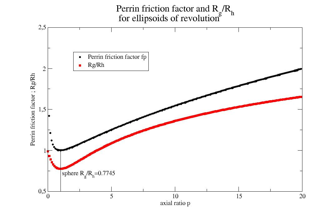
- jscatter.formel.qEwaldSphere(q, wavelength=0.15406, typ=None, N=60)[source]
Points on Ewald sphere with different distributions.
\(q = \vec{k_s} -\vec{k_i} =4\pi/\lambda sin(\theta/2)\) with \(\vec{k_i} =[0,0,1]\) and \(|\vec{k_i}| =2\pi/\lambda\)
Use rotation matrix to rotate to specific orientations.
- Parameters:
- qarray,list
Wavevectors units 1/nm
- wavelengthfloat
Wavelength of radiation, default X-ray K_a.
- Ninteger
Number of points in intervals.
- typ‘cart’,’ring’,’random’ default=’ring’
- Typ of q value distribution on Ewald sphere.
cart : Cartesian grid between -q_max,q_max with N points (odd to include zero).
ring : Given q values with N-points on rings of equal q.
random : N² random points on Ewald sphere between q_min and q_max.
- Returns:
- array3xN [x,y,z] coordinates
Examples
import jscatter as js
import numpy as np
fig = js.mpl.figure(figsize=[8, 2.7],dpi=200)
ax1 = fig.add_subplot(1, 4, 1, projection='3d')
ax2 = fig.add_subplot(1, 4, 2, projection='3d')
ax3 = fig.add_subplot(1, 4, 3, projection='3d')
ax4 = fig.add_subplot(1, 4, 4, projection='3d')
q0 = 2 * np.pi / 0.15406  # Ewald sphere radius |kin|

q = np.r_[0.:2*q0:10j]
qe = js.formel.qEwaldSphere(q)
js.mpl.scatter3d(qe[0],qe[1],qe[2],ax=ax1,pointsize=1)
ax1.set_title('equidistant q')

q = 2*q0*np.sin(np.r_[0.:np.pi:10j]/2)
qe = js.formel.qEwaldSphere(q)
js.mpl.scatter3d(qe[0],qe[1],qe[2],ax=ax2,pointsize=1)
ax2.set_title('equidistant angle')

qe = js.formel.qEwaldSphere(q=[10],N=20,typ='cart')
js.mpl.scatter3d(qe[0],qe[1],qe[2],ax=ax3,pointsize=1)
ax3.set_title('cartesian grid')

qe = js.formel.qEwaldSphere(q=[10,0.5*q0],N=60,typ='random')
fig = js.mpl.scatter3d(qe[0],qe[1],qe[2],ax=ax4,pointsize=1)
ax4.set_title('random min,max')
#fig.savefig(js.examples.imagepath+'/qEwaldSphere.jpg')
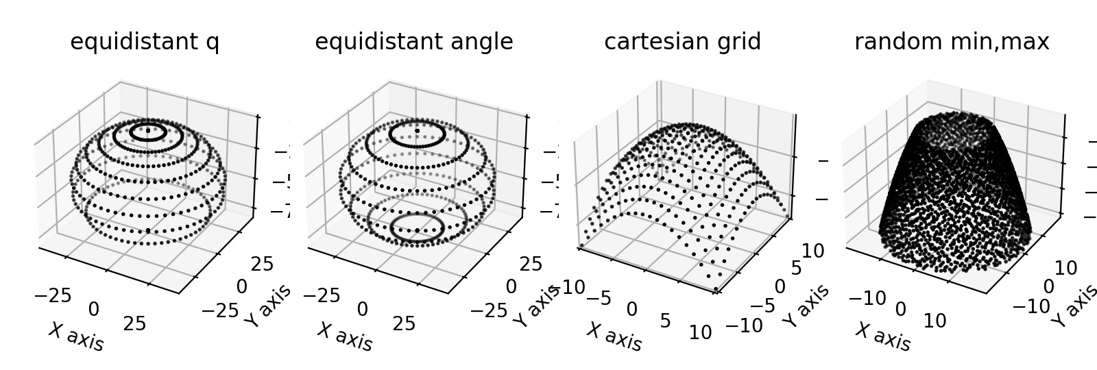
- jscatter.formel.randomPointsInCube(NN, skip=0, dim=3)[source]
N quasi random points in cube of edge 1 based on low-discrepancy sequence.
For numerical integration quasi random numbers are better than random samples as the error drops faster [1]. Here we use the Halton sequence to generate the sequence. Skipping points makes the sequence additive and does not repeat points.
- Parameters:
- NNint
Number of points to generate.
- skipint
Number of points to skip in Halton sequence .
- dimint, default 3
Dimension of the cube.
- Returns:
- array of [x,y,z]
References
Examples
The visual difference between pseudorandom and random in 2D. See [1] for more details.
import jscatter as js
import matplotlib.pyplot as pyplot
fig = pyplot.figure(figsize=(10, 5))
fig.add_subplot(1, 2, 1, projection='3d')
fig.add_subplot(1, 2, 2, projection='3d')
js.sf.randomLattice([2,2],3000).show(fig=fig, ax=fig.axes[0])
fig.axes[0].set_title('random lattice')
js.sf.pseudoRandomLattice([2,2],3000).show(fig=fig, ax=fig.axes[1])
fig.axes[1].set_title('pseudo random lattice \n less holes more homogeneous')
fig.axes[0].view_init(elev=85, azim=10)
fig.axes[1].view_init(elev=85, azim=10)
#fig.savefig(js.examples.imagepath+'/comparisonRandom-Pseudorandom.jpg')
Random cubes of random points in cube.
# random cubes of random points in cube
import jscatter as js
import numpy as np
import matplotlib.pyplot as plt
from mpl_toolkits.mplot3d import Axes3D
fig = plt.figure()
ax = fig.add_subplot(111, projection='3d')
N=30
cubes=js.formel.randomPointsInCube(20)*3
for i,color in enumerate(['b','g','r','y','k']*3):
   points=js.formel.randomPointsInCube(N,skip=N*i).T
   pxyz=points*0.3+cubes[i][:,None]
   ax.scatter(pxyz[0,:],pxyz[1,:],pxyz[2,:],color=color,s=20)
ax.set_xlim([0,3])
ax.set_ylim([0,3])
ax.set_zlim([0,3])
plt.tight_layout()
plt.show(block=False)
#fig.savefig(js.examples.imagepath+'/randomRandomCubes.jpg')
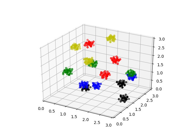
- jscatter.formel.randomPointsOnSphere(NN, r=1, skip=0)[source]
N quasi random points on sphere of radius r based on low-discrepancy sequence.
For numerical integration quasi random numbers are better than random samples as the error drops faster [1]. Here we use the Halton sequence to generate the sequence. Skipping points makes the sequence additive and does not repeat points.
- Parameters:
- NNint
Number of points to generate.
- rfloat
Radius of sphere
- skipint
Number of points to skip in Halton sequence .
- Returns:
- array of [r,phi,theta] pairs in radians
References
Examples
A random sequence of points on sphere surface.
import jscatter as js
import numpy as np
import matplotlib.pyplot as plt
from mpl_toolkits.mplot3d import Axes3D
fig = plt.figure()
ax = fig.add_subplot(111, projection='3d')
for i,color in enumerate(['b','g','r','y']):
   points=js.formel.randomPointsOnSphere(400,skip=400*i)
   points=points[points[:,1]>0,:]
   pxyz=js.formel.rphitheta2xyz(points)
   ax.scatter(pxyz[:,0],pxyz[:,1],pxyz[:,2],color=color,s=20)
ax.set_xlim([-1,1])
ax.set_ylim([-1,1])
ax.set_zlim([-1,1])
fig.axes[0].set_title('random points on sphere (half shown)')
plt.tight_layout()
plt.show(block=False)
#fig.savefig(js.examples.imagepath+'/randomPointsOnSphere.jpg')
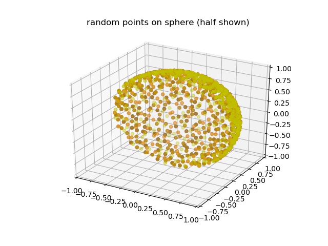
- jscatter.formel.rotationMatrix(vector, angle)[source]
Create a rotation matrix corresponding to rotation around vector v by a specified angle.
\[R = vv^T + cos(a) (I - vv^T) + sin(a) skew(v)\]See Notes for scipy rotation matrix.
- Parameters:
- vectorarray
Rotation around a general vector
- anglefloat
Angle in rad
- Returns:
- array
Rotation matrix
Notes
A convenient way to define more complex rotations is found in scipy.spatial.transform.Rotation . E.g. by Euler angles and returned as rotation matrix
from scipy.spatial.transform import Rotation as Rot
R=Rot.from_euler('YZ',[90,10],1).as_matrix()
References
Examples
Examples show how to use a rotation matrix with vectors.
import jscatter as js
import numpy as np
from matplotlib import pyplot
R=js.formel.rotationMatrix([0,0,1],np.deg2rad(-90))
v=[1,0,0]
# rotated vector
rv=np.dot(R,v)
#
# rotate Fibonacci Grid
qfib=js.formel.fibonacciLatticePointsOnSphere(300,1)
qfib=qfib[qfib[:,2]<np.pi/2,:]                       # select half sphere
qfib[:,2]*=(30/90.)                                  # shrink to cone of 30°
qfx=js.formel.rphitheta2xyz(qfib)                    # transform to cartesian
v = [0,1,0]                                          # rotation vector
R=js.formel.rotationMatrix(v,np.deg2rad(90))        # rotation matrix around v axis
Rfx=np.einsum('ij,kj->ki',R,qfx)                     # do rotation
fig = pyplot.figure()
ax = fig.add_subplot(111, projection='3d')
sc=ax.scatter(qfx[:,0], qfx[:,1], qfx[:,2], s=2, color='r')
sc=ax.scatter(Rfx[:,0], Rfx[:,1], Rfx[:,2], s=2, color='b')
ax.scatter(0,0,0, s=55, color='g',alpha=0.5)
ax.quiver([0],[0],[0],*v,color=['g'])
fig.axes[0].set_title('rotate red points to blue around vector (green)')
pyplot.show(block=False)
# fig.savefig(js.examples.imagepath+'/rotationMatrix.jpg')
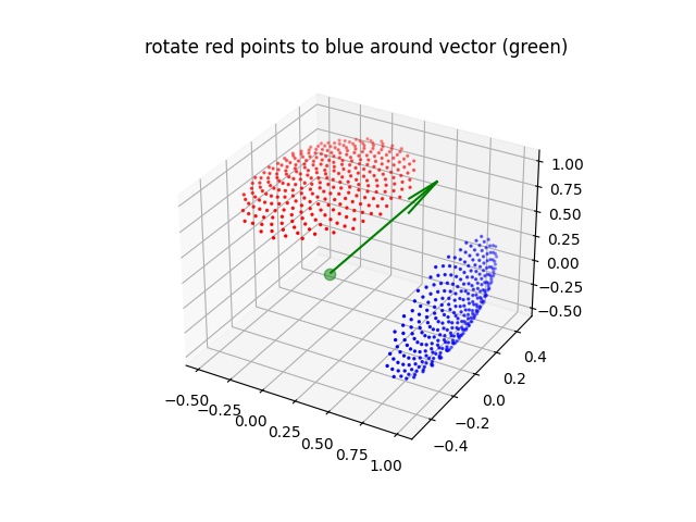
- jscatter.formel.rphitheta2xyz(RPT, transpose=False)[source]
Transformation spherical coordinates [r,phi,theta] to cartesian coordinates [x,y,z].
- Parameters:
- RPTarray Nx3
- Coordinates with [r,phi,theta]
r : float length
phi : float azimuth -pi < phi < pi
theta : float polar angle 0 < theta < pi
- transposebool
Transpose RPT before transformation.
- Returns:
- array Nx3
[x,y,z] coordinates
- jscatter.formel.scatteringFromSizeDistribution(q, sizedistribution, size=None, func=None, weight=None, **kwargs)[source]
Average function assuming one multimodal parameter like bimodal.
Distributions might be mixtures of small and large particles bi or multimodal. For predefined distributions see formel.parDistributedAverage with examples. The weighted average over given sizedistribution is calculated.
- Parameters:
- qarray of float;
Wavevectors to calculate scattering; unit = 1/unit(size distribution)
- sizedistributiondataArray or array
Explicit given distribution of sizes as [ [list size],[list probability]]
- sizestring
Name of the parameter describing the size (may be also something different than size).
- funclambda or function, default beaucage
Function that describes the form factor with first arguments (q,size,…) and should return dataArray with .Y as result as e.g.func=js.ff.sphere.
- kwargs
Any additional keyword arguments passed to for func.
- weightfunction
Weight function dependent on size. E.g. weight = lambda R:rho**2 * (4/3*np.pi*R**3)**2 with V= 4pi/3 R**3 for normalized form factors to account for forward scattering of volume objects of dimension 3.
- Returns:
- dataArray
Columns [q,I(q)]
Notes
We have to discriminate between formfactor normalized to 1 (e.g. beaucage) and form factors returning the absolute scattering (e.g. sphere) including the contrast. The later contains already \(\rho^2 V^2\), the first not.
We need for normalized formfactors P(q) \(I(q) = n \rho^2 V^2 P(q)\) with \(n\) as number density \(\rho\) as difference in average scattering length (contrast), V as volume of particle (~r³ ~ mass) and use \(weight = \rho^2 V(R)^2\)
\[I(q)= \sum_{R_i} [ weight(R_i) * probability(R_i) * P(q, R_i , *kwargs).Y ]\]For a gaussian chain with \(R_g^2=l^2 N^{2\nu}\) and monomer number N (nearly 2D object) we find \(N^2=(R_g/l)^{1/\nu}\) and the forward scattering as weight \(I_0=b^2 N^2=b^2 (R_g/l)^{1/\nu}\)
Examples
The contribution of different simple sizes to Beaucage
import jscatter as js
q=js.loglist(0.01,6,100)
p=js.grace()
# bimodal with equal concentration
bimodal=[[12,70],[1,1]]
Iq=js.formel.scatteringFromSizeDistribution(q=q,sizedistribution=bimodal,
                                            d=3,weight=lambda r:(r/12)**6,func=js.ff.beaucage)
p.plot(Iq,legend='bimodal 1:1 weight ~r\S6 ')
Iq=js.formel.scatteringFromSizeDistribution(q=q,sizedistribution=bimodal,d=3,func=js.ff.beaucage)
p.plot(Iq,legend='bimodal 1:1 weight equal')
# 2:1 concentration
bimodal=[[12,70],[1,5]]
Iq=js.formel.scatteringFromSizeDistribution(q=q,sizedistribution=bimodal,d=2.5,func=js.ff.beaucage)
p.plot(Iq,legend='bimodal 1:5 d=2.5')
p.yaxis(label='I(q)',scale='l')
p.xaxis(scale='l',label='q / nm\S-1')
p.title('Bimodal size distribution Beaucage particle')
p.legend(x=0.2,y=10000)
#p.save(js.examples.imagepath+'/scatteringFromSizeDistribution.jpg')
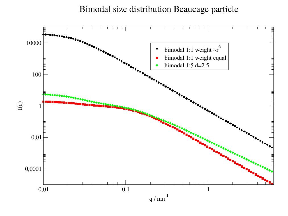
Three sphere sizes:
import jscatter as js
q=js.loglist(0.001,6,1000)
p=js.grace()
# trimodal with equal concentration
trimodal=[[10,50,500],[1,0.01,0.00001]]
Iq=js.formel.scatteringFromSizeDistribution(q=q,sizedistribution=trimodal,size='radius',func=js.ff.sphere)
p.plot(Iq,legend='with aggregates')
p.yaxis(label='I(q)',scale='l',max=1e13,min=1)
p.xaxis(scale='l',label='q / nm\S-1')
p.text(r'minimum \nlargest',x=0.002,y=1e10)
p.text(r'minimum \nmiddle',x=0.02,y=1e7)
p.text(r'minimum \nsmallest',x=0.1,y=1e5)
p.title('trimodal spheres')
p.subtitle('first minima indicated')
#p.save(js.examples.imagepath+'/scatteringFromSizeDistributiontrimodal.jpg')
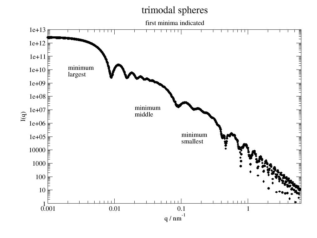
- jscatter.formel.scatteringLengthDensityCalc(composition, density=None, T=293, units='mol', mode='all')[source]
Scattering length density of composites and water with inorganic components for xrays and neutrons.
- Parameters:
- compositionlist of concentration + chemical formula
A string with chemical formula as letter + number and prepended concentration in mol or mmol. E.g. ‘0.1C3H8O3’ or ‘0.1C3H1D7O3’ for glycerol and deuterated glycerol (‘D’ for deuterium).
For single atoms append 1 to avoid confusion. Fractional numbers allowed, but think of meaning (Isotope mass fraction??)
For compositions use a list of strings preceded by mass fraction or concentration in mol of component. This will be normalized to total amount
Examples:
[‘4.5H2O1’,’0.5D2O1’] mixture of 10% heavy and 90% light water.
[‘1.0h2o’,’0.1c3h8o3’] for 10% mass glycerol added to 100% h2o with units=’mass’
[‘55000H2O1’,’50Na3P1O4’,’137Na1Cl1’] for a 137mMol NaCl +50mMol phophate H2O buffer (1l is 55000 mM H2O)
[‘1Au1’] gold with density 19.302 g/ml
Remember to adjust density.
- densityfloat, default=None
Density in g/cm**3 = g/ml.
If not given function waterdensity is tried to calculate the solution density with inorganic components. In this case ‘h2o1’ and/or ‘d2o1’ need to be in composition.
Density can be measure by weighting a volume from pipette (lower accuracy) or densiometry (higher accuracy).
Estimate for deuterated compounds from protonated density according to additional D. Mass change is given with mode=’all’.
- units‘mol’
Anything except ‘mol’ prepended unit is mass fraction (default). ‘mol’ prepended units is mol and mass fraction is calculated as mass=[mol]*mass_of_molecule e.g. 1l Water with 123mmol NaCl [‘55.5H2O1’,’0.123Na1Cl1’]
- mode
‘xsld’ xray scattering length density in nm**-2
‘edensity’ electron density in e/nm**3
‘ncohsld’ coherent scattering length density in nm**-2
‘incsld’ incoherent scattering length density in nm**-2
‘num’ number density of components in 1/nm**3
‘all’ [xsld, edensity, ncohsld, incsld, masses, masses full protonated, masses full deuterated, d2o/h2o mass fraction, d2o/h2o mol fraction]
‘all2’ [xsld, edensity, ncohsld, incsld, masses, masses full protonated, masses full deuterated, d2o/h2o number fraction,number densities in 1/nm³, density in g/cm³]
- Tfloat, default=293
Temperature in °K
- Returns:
- float, list
sld corresponding to mode
Notes
edensity=be*massdensity/weightpermol*sum_atoms(numberofatomi*chargeofatomi)
be = scattering length electron =µ0*e**2/4/pi/m=2.8179403267e-6 nm
masses, masses full protonated, masses full deuterated for each chemical in composition.
In mode ‘all’ the masses can be used to calc the deuterated density if same volume is assumed. e.g. fulldeuterated_density=protonated_density/massfullprotonated*massfulldeuterated
For density reference of H2O/D2O see waterdensity.
Examples
# 5% D2O in H2O with 10% mass NaCl
js.formel.scatteringLengthDensityCalc(['9.5H2O1','0.5D2O1','1Na1Cl1'],units='mass')
# protein NaPi buffer in D2O prevalue in mmol; 55507 mmol H2O is 1 liter.
# because of the different density the sum of number density is not 55.507 mol but 55.191 mol.
js.formel.scatteringLengthDensityCalc(['55507D2O1','50Na3P1O4','137Na1Cl1'])
# silica
js.formel.scatteringLengthDensityCalc('1Si1O2',density=2.65)
# gold
js.formel.scatteringLengthDensityCalc(['1Au1'],density=19.32)
# PEG1000
js.formel.scatteringLengthDensityCalc(['1C44H88O23'],density=1.21)
- jscatter.formel.schulzDistribution(r, mean, sigma)[source]
Schulz (or Gamma) distribution for polymeric particles/chains.
Distribution describing a polymerization like radical polymerization:
constant number of chains growth till termination.
concentration of active centers constant.
start of chain growth not necessarily at the same time.
In polymer physics sometimes called Schulz-Zimm distribution. Same as Gamma distribution.
- Parameters:
- rarray
Distribution variable such as relative molecular mass or degree of polymerization, number of monomers.
- meanfloat
Mean \(<r>\)
- sigmafloat
Width as standard deviation \(s=\sqrt{<r^2>-<r>^2}\) of the distribution. \(z = (<r>/s)^2 -1 < 600\)
- Returns:
- dataArrayColumns [x,p]
.z ==> z+1 = k is degree of coupling = number of chain combined to dead chain in termination reaction
z = (<r>/s)² -1
Notes
The Schulz distribution [1]
\[h(r) = \frac{(z+1)^{z+1}r^z}{mean^{z+1}\Gamma(z+1)}e^{-(z+1)\frac{r}{mean}}\]alternatively with \(a=<r>^2/s^2\) and \(b=a/<r>\)
\[h(r) = \frac{b^a r^(a-1)}{\Gamma(a)}e^{-br}\]Normalized to \(\int h(r)dr=1\).
- Nth order average \(<r>^n = \frac{z+n}{z+1} <r>\)
number average \(<r>^1 = <r>\)
weight average \(<r>^2 = \frac{z+2}{z+1} <r>\)
z average \(<r>^3 = \frac{z+3}{z+1} <r>\)
References
[1]Schulz, G. V. Z. Phys. Chem. 1939, 43, 25
[2]Theory of dynamic light scattering from polydisperse systems S. R. Aragón and R. Pecora The Journal of Chemical Physics, 64, 2395 (1976)
Examples
import jscatter as js
import numpy as np
N=np.r_[1:200]
p=js.grace(1.4,1)
p.multi(1,2)
m=50
for i,s in enumerate([10,20,40,50,75,100,150],1):
    SZ = js.formel.schulzDistribution(N,mean=m,sigma=s)
    p[0].plot(SZ.X/m,SZ.Y,sy=0,li=[1,3,i],le=f'sigma/mean={s/m:.1f}')
    p[1].plot(SZ.X/m,SZ.Y*SZ.X,sy=0,li=[1,3,i],le=f'sigma/mean={s/m:.1f}')
p[0].xaxis(label='N/mean')
p[0].yaxis(label='h(N)')
p[0].subtitle('number distribution')
p[1].xaxis(label='N/mean')
p[1].yaxis(label='N h(N)')
p[1].subtitle('mass distribution')
p[1].legend(x=2,y=1.5)
p[0].title('Schulz distribution')
#p.save(js.examples.imagepath+'/schulzZimm.jpg')
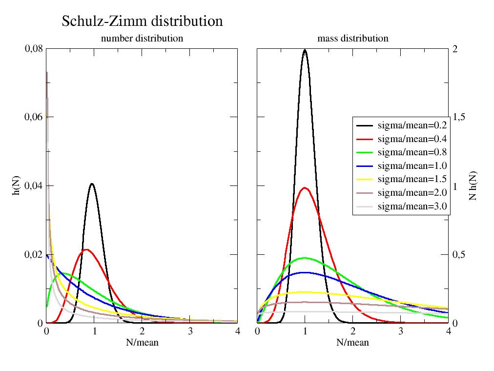
- jscatter.formel.sedimentationCoefficient(M, partialVol=None, density=None, visc=None)[source]
Sedimentation coefficient of a sphere in a solvent.
\(S = M (1-\nu \rho)/(N_A 6\pi \eta R)\) with \(V = 4/3\pi R^3 = \nu M\)
- Parameters:
- Mfloat
Mass of the sphere or protein in units Da.
- partialVolfloat
Partial specific volume \(\nu\) of the particle in units ml/g = l/kg. Default is 0.73 ml/g for proteins.
- densityfloat
Density \(\rho\) of the solvent in units g/ml=kg/l. Default is H2O at 293.15K
- viscfloat
Solvent viscosity \(\eta\) in Pas. Default H2O at 293.15K
- Returns:
- float
Sedimentation coefficient in units Svedberg (1S = 1e-13 sec )
- jscatter.formel.sedimentationProfile(t=1000.0, rm=48, rb=85, number=100, rlist=None, c0=0.01, S=None, Dt=None, omega=246, Rh=10, temp=293, densitydif=0.37, visc='h2o')[source]
Concentration profile of sedimenting particles in a centrifuge including bottom equilibrium distribution.
Approximate solution to the Lamm equation including the bottom equilibrium distribution which is not included in the Faxen solution. This calculates equ. 28 in [1]. Results in particle concentration profile between rm and rb for time t with a equal distribution at the start.
- Parameters:
- tfloat or list
Time after centrifugation start in seconds. If list, a dataList for all times is returned.
- rmfloat
Axial position of meniscus in mm.
- rbfloat
Axial position of bottom in mm.
- numberint
Number of points between rm and rb to calculate.
- rlistlist of float
Explicit list of positions where to calculate e.g.to zoom bottom.
- c0float
Initial concentration in cell; just a scaling factor.
- Sfloat
Sedimentation coefficient in units Svedberg; 82 S is r=10 nm protein in H2O at T=20C.
- Dtfloat
Translational diffusion coefficient in m**2/s; 1.99e-11 is r=10 nm particle.
- omegafloat
Radial velocity rounds per second; 14760rpm = 246 rps = 1545 rad/s is 20800g in centrifuge fresco 21.
- Rhfloat
Hydrodynamic radius in nm ; if given the Dt and s are calculated from this.
- densitydiffloat
Density difference between solvent and particle in g/ml; Protein in ‘h2o’ => 1.37-1.= 0.37 g/cm**3.
- viscfloat, ‘h2o’, ‘d2o’
Viscosity of the solvent in Pas. (H2O ~ 0.001 Pa*s =1 cPoise) If ‘h2o’ or ‘d2o’ the corresponding viscosity at given temperature is used.
- tempfloat
temperature in K.
- Returns:
- dataArray, dataList
Concentration profile Columns [position in [mm]; conc ; conc_meniscus_part; conc_bottom_part]
Notes
From [1]:”The deviations from the expected results are smaller than 1% for simulated curves and are valid for a great range of molecular masses from 0.4 to at least 7000 kDa. The presented approximate solution, an essential part of LAMM allows the estimation of s and D with an accuracy comparable to that achieved using numerical solutions, e.g the program SEDFIT of Schuck et al.”
Default values are for Heraeus Fresco 21 at 21000g.
References
Examples
Cleaning from aggregates by sedimantation. Sedimentation of protein (R=2 nm) with aggregates of 100nm size.
import numpy as np
import jscatter as js
t1=np.r_[60:1.15e3:11j]  # time in seconds

# open plot()
p=js.grace(1.5,1.5)
p.multi(2,1)

# calculate sedimentation profile for two different particles
# data correspond to Fresco 21 with dual rotor
# default is solvent='h2o',temp=293
g=21000. # g # RZB number
omega=g*246/21000
D2nm=js.formel.sedimentationProfile(t=t1,Rh=2,densitydif=0.37, number=1000)
D50nm=js.formel.sedimentationProfile(t=t1,Rh=50,densitydif=0.37, number=1000)

# plot it
p[0].plot(D2nm,li=[1,2,-1],sy=0,legend='t=$time s' )
p[1].plot(D50nm,li=[1,2,-1],sy=0,legend='t=$time s' )

# pretty up
p[0].yaxis(min=0,max=0.05,label='concentration')
p[1].yaxis(min=0,max=0.05,label='concentration')
p[1].xaxis(label='position mm')
p[0].xaxis(label='')
p[0].text(x=70,y=0.04,string=r'R=2 nm \nno sedimantation')
p[1].text(x=70,y=0.04,string=r'R=50 nm \nfast sedimentation')
p[0].legend(x=42,y=0.05,charsize=0.5)
p[1].legend(x=42,y=0.05,charsize=0.5)
p[0].title('Concentration profile in first {0:} s'.format(np.max(t1)))
p[0].subtitle('2nm and 50 nm particles at 21000g ')
#p.save(js.examples.imagepath+'/sedimentation.jpg')
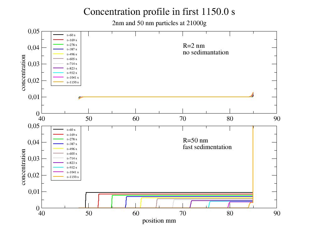
Sedimentation (up concentration) of unilamellar liposomes of DOPC. The density of DOPC is about 1.01 g/ccm in water with 1 g/ccm. Lipid volume fraction is 33% for 50nm radius (10% for 200 nm) for a bilayer thickness of 6.5 nm.
import numpy as np
import jscatter as js

t1=np.r_[100:6e3:11j]  # time in seconds

# open plot()
p=js.grace(1.5,1.5)
p.multi(2,1)

# calculate sedimentation profile for two different particles
# data correspond to Fresco 21 with dual rotor
# default is solvent='h2o',temp=293
g=21000. # g # RZB number
omega=g*246/21000
D100nm=js.formel.sedimentationProfile(t=t1,Rh=50,c0=0.05,omega=omega,rm=48,rb=85,densitydif=0.003)
D400nm=js.formel.sedimentationProfile(t=t1,Rh=200,c0=0.05,omega=omega,rm=48,rb=85,densitydif=0.001)

# plot it
p[0].plot(D100nm,li=[1,2,-1],sy=0,legend='t=$time s' )
p[1].plot(D400nm,li=[1,2,-1],sy=0,legend='t=$time s' )

# pretty up
p[0].yaxis(min=0,max=0.2,label='concentration')
p[1].yaxis(min=0,max=0.2,label='concentration')
p[1].xaxis(label='position mm')
p[0].xaxis(label='')
p[0].text(x=70,y=0.15,string='D=100 nm')
p[1].text(x=70,y=0.15,string='D=400 nm')
p[0].legend(x=42,y=0.2,charsize=0.5)
p[1].legend(x=42,y=0.2,charsize=0.5)
p[0].title('Concentration profile in first {0:} s'.format(np.max(t1)))
p[0].subtitle('at 21000g ')
- jscatter.formel.sedimentationProfileFaxen(t=1000.0, rm=48, rb=85, number=100, rlist=None, c0=0.01, s=None, Dt=1.99e-11, w=246, Rh=10, visc='h2o', temp=293, densitydif=None)[source]
Faxen solution to the Lamm equation of sedimenting particles in centrifuge; no bottom part.
Bottom equillibrium distribution is not in Faxen solution included. Results in particle distribution along axis for time t.
- Parameters:
- tfloat
Time after start in seconds. If list, results at these times is given as dataList.
- rmfloat
Axial position of meniscus in mm.
- rbfloat
Axial position of bottom in mm.
- rlistarray, optional
Explicit list of radial values to use between rm=max(rlist) and rb=min(rlist)
- numberinteger
Number of points between rm and rb to calculate.
- c0float
Initial concentration in cell; just a scaling factor.
- sfloat
Sedimentation coefficient in Svedberg; 77 S is r=10 nm particle in H2O.
- Dtfloat
Translational diffusion coefficient in m**2/s; 1.99e-11 is r=10 nm particle.
- wfloat
Radial velocity rounds per second; 246 rps=2545 rad/s is 20800g in centrifuge fresco 21.
- Rhfloat
Hydrodynamic radius in nm ; if given Dt and s are calculated from Rh.
- viscfloat, ‘h2o’,’d2o’
Viscosity in units Pas. If ‘h2o’ or ‘d2o’ the corresponding viscosity at given temperature is used.
- densitydiffloat
Density difference between solvent and particle in g/ml. Protein in ‘h2o’=> is used =>1.37-1.= 0.37 g/cm**3
- tempfloat
temperature in K.
- Returns:
- dataArray, dataList
Concentration distribution : dataArray, dataList
.pelletfraction is the content in pellet as fraction already diffused out .rmeniscus
Notes
Default values are for Heraeus Fresco 21 at 21000g.
References
[1]Über eine Differentialgleichung aus der physikalischen Chemie. Faxén, H. Ark. Mat. Astr. Fys. 21B:1-6 (1929)
Close and unlink shared memory array.
- Parameters:
- shmsharedMemory
SharedMemory created by shared_create.
Create shared memory array before sending into pool of workers or usage in doForList .
Creation of shared memory for numpy arrays as described in https://docs.python.org/3/library/multiprocessing.shared_memory.html#module-multiprocessing.shared_memory
- Parameters:
- ararray
Numpy array to copy into a shared memory array.
- copybool
Copy data or not.
- Returns:
- sharedMemory, tuple with (namestring, ar.shape, ar.dtype)
sharedMemory is the shared memory
tuple is information to recover the original array, name is a unique identifier The tuple needs to be passed to the function in doForList instead of ar.
Notes
This function (with
shared_recover()andshared_close()) is more for experts.The speedup e.g. in cloudScattering is not huge as the main time is consumed in calculations.
Also creating shared memory (~8ms for 1e6x3 array) takes around the same time as numpy array pickling (~3ms) for transfer to a pool of workers. Inside the pool the recover is much faster (~ 47µs) compared to unpickling (1.2.ms)
The speedup will be more important if e.g. the qlist (see example) is huge and the calculations are short. In this case data transfer will be more important than the calculation.
Examples
Take the following and paste it to script.py In a python shell do run scripy.py In this way the fucntions are defined and can be accessed.
Using this in imported scripts is not necessary.
import jscatter as js
import numpy as np

def model(q, ar_id):
   # recover the array from shared memory
   ar_sh, ar = js.formel.shared_recover(ar_id)

   # here we do a difficult calculation for a single q value but the whole array
   sum = np.sum(q*ar)
   ar_sh.close()
   return sum

if __name__ == '__main__':
    __spec__ = None
    qlist=np.r_[0.1:10:0.1]

    # example grid with about 1e6 points
    cloud = js.ff.superball(1, 10, p=2, nGrid=100, returngrid=True).XYZ

    # transfer large grid to shared memory
    cloud_sh, cloud_id = js.formel.shared_create(cloud)

    # do the calculation for a qlist values
    res = js.formel.doForList(model, qlist, loopover='q', ar=cloud_id)

    # always free the shared memory (close and unlink)
    js.formel.shared_close(cloud_sh)
Recover shared memory array inside a function evaluated in a pool of workers.
- Parameters:
- shm_idtuple created by shared_create
- Returns:
- sharedMemory, ndarray
- jscatter.formel.simpleQuadratureSimpson(funktion, lowlimit, uplimit, parname, weights=None, tol=1e-06, rtol=1e-06, **kwargs)[source]
Integrate a scalar function over one of its parameters with weights using the adaptive Simpson rule. Shortcut sQS.
Integrate by adaptive Simpson integration for scalar function.
- Parameters:
- funktionfunction
function to integrate
- lowlimit,uplimitfloat
interval to integrate
- parnamestring
parname to integrate
- weightsndarray shape(2,N),default=None
Weights for integration along parname as a Gaussian with a<weights[0]<b and weights[1] contains weight values.
Missing values are linear interpolated (faster). If None equal weights are used.
- tol,rtolfloat, default=1e-6
- Relative error for intervals or absolute integral error to stop integration.
- kwargs
additional parameters to pass to funktion if parname is in kwargs it is overwritten
- Returns:
- float
Notes
What is the meaning of tol in Simpson method? See parQuadratureSimpson.
References
Examples
distrib =scipy.stats.norm(loc=1,scale=0.2)
x=np.linspace(0,1,1000)
pdf=np.c_[x,distrib.pdf(x)].T
# define function
f1=lambda x,p1,p2,p3:js.dA(np.c_[x,x*p1+x*x*p2+p3].T)
# calc the weighted integral
result=js.formel.parQuadratureSimpson(f1,0,1,parname='p2',weights=pdf,tol=0.01,p1=1,p3=1e-2,x=x)
# something simple should be 1
js.formel.simpleQuadratureSimpson(js.formel.gauss,-10,10,'x',mean=0,sigma=1)
- jscatter.formel.smooth(data, windowlen=7, window='flat')[source]
Smooth data by convolution with window function or fft/ifft.
Smoothing based on position ignoring information on .X.
- Parameters:
- dataarray, dataArray
Data to smooth. If is dataArray the .Y is smoothed and returned.
- windowlenint, default = 7
The length/size of the smoothing window; should be an odd integer. Smaller 3 returns unchanged data. For ‘fourier’ the high frequency cutoff is 2*size_data/windowlen.
- window‘hann’, ‘hamming’, ‘bartlett’, ‘blackman’,’gaussian’,’fourier’,’flattop’ default =’flat’
- Type of window/smoothing.
‘flat’ will produce a moving average smoothing.
‘gaussian’ normalized Gaussian window with sigma=windowlen/7.
‘fourier’ cuts high frequencies above cutoff frequency between rfft and irfft.
- Returns:
- array (only the smoothed array)
Notes
- ‘hann’, ‘hamming’, ‘bartlett’, ‘blackman’,’gaussian’, ‘flat’ :
These methods convolve a scaled window function with the signal. The signal is prepared by introducing reflected copies of the signal (with the window size) at both ends so that transient parts are minimized in the beginning and end part of the output signal. Adapted from SciPy/Cookbook.
- fourier :
The real valued signal is mirrored at left side, Fourier transformed, the high frequencies are cut and the signal is back transformed. This is the simplest form as a hard cutoff frequency is used (ideal low pass filter) and may be improved using a specific window function in frequency domain.
rft = np.fft.rfft(np.r_[data[::-1],data])
rft[int(2*len(data)/windowlen):] = 0
smoothed = np.fft.irfft(rft)
Examples
Usage:
import jscatter as js
import numpy as np
t=np.r_[-5:5:0.01]
data=np.sin(t)+np.random.randn(len(t))*0.1
y=js.formel.smooth(data)  # 1d array
#
# smooth dataArray and replace .Y values.
data2=js.dA(np.vstack([t,data]))
data2.Y=js.formel.smooth(data2, windowlen=40, window='gaussian')
Comparison of some filters:
import jscatter as js
import numpy as np
t=np.r_[-5:5:0.01]
data=js.dA(np.vstack([t,np.sin(t)+np.random.randn(len(t))*0.1]))
p=js.grace()
p.multi(4,2)
windowlen=31
for i,window in enumerate(['flat','gaussian','hann','fourier']):
    p[2*i].plot(data,sy=[1,0.1,6],le='original + noise')
    p[2*i].plot(t,js.formel.smooth(data,windowlen,window),sy=[2,0.1,4],le='filtered')
    p[2*i].plot(t,np.sin(t),li=[1,0.5,1],sy=0,le='noiseless')
    p[2*i+1].plot(data,sy=[1,0.1,6],le='original noise')
    p[2*i+1].plot(t,js.formel.smooth(data,windowlen,window),sy=[2,0.1,4],le=window)
    p[2*i+1].plot(t,np.sin(t),li=[1,2,1],sy=0,le='noiseless')
    p[2*i+1].text(window,x=-2.8,y=-1.2)
    p[2*i+1].xaxis(min=-3,max=-1,)
    p[2*i+1].yaxis(min=-1.5,max=-0.2,ticklabel=[None,None,None,'opposite'])
    p[2*i].yaxis(label='y')
p[0].legend(x=10,y=4.5)
p[6].xaxis(label='x')
p[7].xaxis(label='x')
p[0].title(f'Comparison of smoothing windows')
p[0].subtitle(f'with windowlen {windowlen}')
#p.save(js.examples.imagepath+'/smooth.jpg')
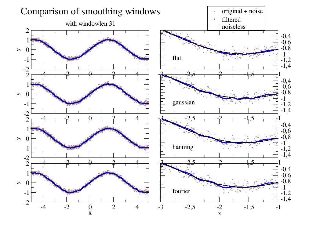
- jscatter.formel.sphereAverage(funktion, relError=300, *args, **kwargs)[source]
Vectorized spherical average of funktion, parallel or non-parallel.
A Fibonacci lattice or Monte Carlo integration with pseudo random grid is used.
- Parameters:
- funktionfunction
Function to evaluate. Funktion first argument gets cartesian coordinate [x,y,z] of point on unit sphere.
- relErrorfloat, default 300
Determines how points on sphere are selected
>1 Fibonacci Lattice with relError*2+1 points
0<1 Pseudo random points on sphere (see randomPointsOnSphere).
Stops if relative improvement in mean is less than relError (uses steps of 40 or (20ncpu) new points). Final error is (stddev of N points) /sqrt(N) as for Monte Carlo methods even if it is not a correct 1-sigma error in this case.
This has to be used with care as convergence might be slow if std is intrinsically large in calculated values.
- ncpuint, optional
Number of cpus in the pool if started as main process (otherwise single process).
not given or 0 -> default, all cpus are used
int>0 min (ncpu, mp.cpu_count)
int<0 ncpu not to use
Please check if multiprocessing is really useful. For simple calculations it’s faster not to use it (avoiding pickle overhead). The below first example is around 10times faster on a single core (ncpu=1). Think about passPoints.
- passPointsbool
If the function accepts a Nx3 array of points these will be passed instead of single points. The function return value should index the points result in axis 0. This might speed up dependent on the function (e.g. formfactor prism) .
Sets ncpu=1 .
- arg,kwargs
forwarded to function
- Returns:
- array
Values from function and appended Monte Carlo error estimates.
If an array of values is returned in function, the result is also an array with double size.
To separate use values, error = res.reshape(2,-1)
If list of array is returned a list is returned with values and error.
Notes
Works also on single core machines and with single process (avoiding creation of a pool of workers).
For integration over a continuous function as a form factor in scattering the random points are not statistically independent. Think of neighboring points on an isosurface which are correlated and therefore the standard deviation is biased. In this case the Fibonacci lattice is the better choice as the standard deviation in a random sample is not a measure of error but more a measure of the differences on the isosurface.
Examples
Parallel sphere average
Conversion to rpt coordinates and sum results in average value of these coordinate in result. Error of radius is machine precision, phi,theta errors are typical Monte Carlo error
The function should be used in a module to work on Windows. Usage in a module is recomended like demonstrated in
doForList()import jscatter as js def f(x,r): # return a list of values to integrate return [js.formel.xyz2rphitheta(x)*r] val, error = js.formel.sphereAverage(f,relError=500,r=1) # => [1, 0, pi/2 ] js.formel.sphereAverage(f,relError=0.01,r=1)
import jscatter as js
import numpy as np

def fp(singlepoint):
   # return a list of values to integrate
   return js.formel.xyz2rphitheta(singlepoint)[1:]

val,error = js.formel.sphereAverage(fp,relError=500).reshape(2,-1)
val,error = js.formel.sphereAverage(fp,relError=0.1).reshape(2,-1)
Pass all points to one process, not parallel. For such a simple function this is faster.
def fps(allpoints,r):
   res = js.formel.xyz2rphitheta(allpoints)
   return res

val,error =  js.formel.sphereAverage(fps,r=1,passPoints=1).reshape(2,-1)
- jscatter.formel.viscosity(mat='h2o', T=293.15)[source]
Viscosity of pure solvents. For buffer solvents use bufferviscosity.
- Parameters:
- matstring ‘h2o’,’d2o’,’toluol’,’methylcyclohexan’, default h2o
Solvent
- Tfloat
Temperature T in Kelvin default 293K
- Returns:
- float
viscosity in Pa*s
water H2O ~ 0.001 Pa*s =1 cPoise # Poise=0.1 Pa*s
References
[1]The Viscosity of Toluene in the Temperature Range 210 to 370 K M. J. Assael, N.K. Dalaouti, J.H., Dymond International Journal of Thermophysics, Vol. 21,291 No. 2, 2000 # accuracy +- 0.4 % laut paper Max error von Experiment data
[2]Thermal Offset Viscosities of Liquid H2O, D2O, and T2O C. H. Cho, J. Urquidi, S. Singh, and G. Wilse Robinson J. Phys. Chem. B 1999, 103, 1991-1994
- jscatter.formel.voigt(x, center=0, fwhm=1, lg=1, asym=0, amplitude=1)[source]
Voigt function for peak analysis (normalized).
The Voigt function is a convolution of gaussian and lorenzian shape peaks for peak analysis. The Lorenzian shows a stronger contribution outside FWHM with a sharper peak. Asymmetry of the shape can be added by a sigmoidal change of the FWHM [2].
- Parameters:
- xarray
Axis values.
- centerfloat
Center of the distribution.
- fwhmfloat
Full width half maximum of the Voigt function.
- lgfloat, default = 1
Lorenzian/gaussian fraction of both FWHM, describes the contributions of gaussian and lorenzian shape.
lorenzian/gaussian >> 1 lorenzian,
lorenzian/gaussian ~ 1 central part gaussian, outside lorenzian wings
lorenzian/gaussian << 1. gaussian
- asymfloat, default=0
Asymmetry factor in sigmoidal as \(fwhm_{asym} = 2*fwhm/(1+np.exp(asym*(x-center)))\) . For a=0 the Voigt is symmetric.
- amplitudefloat, default = 1
amplitude
- Returns:
- dataArray
.center
.sigma
.gamma
.fwhm
.asymmetry
.lorenzianOverGaussian (lg)
Notes
The Voigt function is a convolution of Gaussian and Lorentz functions
\[G(x;\sigma) = e^{-x^2/(2\sigma^2)}/(\sigma \sqrt{2\pi})\ and \ L(x;\gamma) = \gamma/(\pi(x^2+\gamma^2))\]resulting in
\[V(x;\sigma,\gamma)=\frac{\operatorname{Re}[w(z)]}{\sigma\sqrt{2 \pi}}\]with \(z=(x+i\gamma)/(\sigma\sqrt{2})\) and \(Re[w(z)]\) is the real part of the Faddeeva function.
\(\gamma\) is the Lorentz fwhm width and \(fwhm=(2\sqrt{2\ln 2})\sigma\) the Gaussian fwhm width.
The FWHM in Lorentz and Gaussian dependent on the fwhm of the Voigt function is \(fwhm_{Gauss,Lorentz} \approx fwhm / (0.5346 lg + (0.2166 lg^2 + 1)^{1/2})\) (accuracy 0.02%).
References
[2]A simple asymmetric lineshape for fitting infrared absorption spectra Aaron L. Stancik, Eric B. Brauns Vibrational Spectroscopy 47 (2008) 66–69
[3]Empirical fits to the Voigt line width: A brief review Olivero, J. J.; R. L. Longbothum Journal of Quantitative Spectroscopy and Radiative Transfer. 17, 233–236. doi:10.1016/0022-4073(77)90161-3
- jscatter.formel.watercompressibility(d2ofract=1, T=278, units='psnmg')[source]
Isothermal compressibility of H2O and D2O mixtures.
Compressibility \(\kappa\) in units ps²nm/g or in 1/bar. Linear mixture according to d2ofract.
- Parameters:
- d2ofractfloat, default 1
Fraction D2O
- Tfloat, default 278K
Temperature in K
- unitsstring ‘psnmg’
ps^2*nm/(g/mol) or 1/bar
- Returns:
- float
Notes
For the structure factor e.g. of water one finds in agreement to literature
\[S(0) = kT n \kappa = 0.064\]- with thermal energy kT and number density n,
\(n = 55.5mol/l = 33.42 /nm³\),
\(kT=300K*1.380649e^{-23} J/K = 414e^{-23} kgm²/s² = 414e^{-26} g nm²/ps²\)
\(\kappa(300K)=4.625e20 g/nm/ps²\)
References
[1]Isothermal compressibility of Deuterium Oxide at various Temperatures Millero FJ and Lepple FK Journal of chemical physics 54,946-949 (1971) http://dx.doi.org/10.1063/1.1675024
[2]Precise representation of volume properties of water at one atmosphere G. S. Kell J. Chem. Eng. Data, 1967, 12 (1), pp 66–69 http://dx.doi.org/10.1021/je60032a018
Examples
import jscatter as js
n = js.formel.waterdensity('h2o1',T=300) * 1000/18 *6.023e23/1e24
ka = js.formel.watercompressibility(T=300)
kT = 300*1.380649e-26
S0 = kT*n*ka  # => 0.06388
- jscatter.formel.waterdensity(composition, T=293.15, units='mol', showvalidity=False)[source]
Density of water with inorganic substances (salts).
Solvent with composition of H2O and D2O and additional inorganic components at temperature T. Ternary solutions allowed. Units are mol
- Parameters:
- compositionlist of compositional strings
Compositional string of chemical formula as ‘float’+’chemical char’ + integer - First float is content in mol (is later normalized to sum of contents) - chemical letter + number of atoms in formula (single atoms append 1 ,fractional numbers allowed)
'h2o1' or 'd2o1' light and heavy water with 'd1' for deuterium
'c3h8o3' or 'c3h1d7o3' partial deuterated glycerol
['55.55h2o1','2.5Na1Cl1'] for 2.5 mol NaCl added to  1l h2o (55.55 mol)
['20H2O1','35.55D2O1','0.1Na1Cl1'] h2o/d2o mixture with 100mMol NaCl
- unitsdefault=’mol’
Anything except ‘mol’ unit is mass fraction ‘mol’ units is mol and mass fraction is calculated as mass=[mol]*mass_of_molecule e.g. 1l Water with 123mM NaCl [‘55.5H2O1’,’0.123Na1Cl1’]
- Tfloat, default=293.15
temperature in K
- showvaliditybool, default False
Show additionally validity range for temperature and concentration according to [4]. - Temperature range in °C - concentration in wt % or up to a saturated solution (satd) - error in 1/100 % see [4].
- Returns:
- float
Density in g/ml
Notes
D2O maximum density 1.10596 at T=273.15+11.23 K [1] .
For mixtures of H2O/D2O molar volumes add with an accuracy of about 2e-4 cm**3/mol compared to ~18.015 cm**3/mol molar volume [3].
Additional densities of binary aqueous solutions [4].
Water number density
# 55.5079 mol with 18.015 g/mol
js.formel.waterdensity('1H2O1', T=273+4)*1000/18.015
References
[1]The dilatation of heavy water K. Stokland, E. Ronaess and L. Tronstad Trans. Faraday Soc., 1939,35, 312-318 DOI: 10.1039/TF9393500312
[2]Effects of Isotopic Composition, Temperature, Pressure, and Dissolved Gases on the Density of Liquid Water George S. Kell JPCRD 6(4) pp. 1109-1131 (1977)
[3]Excess volumes for H2O + D2O liquid mixtures Bottomley G Scott R Australian Journal of Chemistry 1976 vol: 29 (2) pp: 427
availible components:
h2o1 d2o1
TRIS c4h11n1o3
TABS c8h19n1o6s1

     ag1cl104     ag1n1o3      al1cl3012    al1n3o9      al2s3o12     ba1br2
 ba1cl2       ba1cl2o6     ba1i2        ba1n2o6      c4h11n1o3    c8h19n1o6s1
 ca1br2       ca1cl2       ca1i2        ca1n2o6      cd1br2       cd1c12
 cd1i2        cd1n2o6      cd1so4       co1n2o6      co1s1o4      cs1br1
 cs1cl1       cs1f1        cs1i1        cs1n1o3      cs2s1o4      cu1cl2
 cu1n2o6      cu1s1o4      dy1cl3       er1cl3       fe1cl3       fe1s1o4
 gd1cl3       h1br1        h1cl1        h1cl104      h1i1         h1n1o3
 h2s1o4       h3b103       h3p1o4       hg1c2n2      hg1cl2       k1ag1c2n2
 k1al1s2o8    k1br1        k1br1o3      k1cl1        k1cl103      k1cl104
 k1f1         k1h1c1o3     k1h1s1o4     k1h2p1o4     k1i1         k1i103
 k1mn1o4      k1n1o2       k1n1o3       k1n3         k1o1h1       k1s1c1n1
 k1tart1      k2c1o3       k2cr104      k2cr207      k2s1o4       k3co1c6n6
 k3fe1c6n6    k4fe1c6n6    k4mo1c8n8    la1cl3       li1br1       li1cl1
 li1cl104     li1i1        li1n1o3      li1o1h1      li2s1o4      mg1br2
 mg1br206     mg1cl2       mg1cl2o8     mg1i2        mg1n2o6      mg1s1o4
 mn1cl1       mn1s1o4      n1h3         n1h40x1      n1h4ac1      n1h4al1s2o8
 n1h4cl1      n1h4cl104    n1h4fe1s2o8  n1h4h1s1o4   n1h4h2p1o4   n1h4i1
 n1h4n1o3     n2h8ni1s2o8  n2h8s1o4     n2s203       na1ac1       na1br1
 na1br1o3     na1cl1       na1cl103     na1cl104     na1f1        na1form1
 na1h1s1o4    na1h2p1o4    na1i1        na1i103      na1k1tart1   na1mn104
 na1n1o2      na1n1o3      na1n3        na1o1h1      na1ox1       na1s1c1n1
 na1tart1     na2b407      na2c1o3      na2cr1o4     na2cr207     na2h1p1o4
 na2mo104     na2s1        na2s103      na2s1o4      na2w104      na3p1o4
 na4p207      na5p307      nd1cl3       ni1cl2       ni1n2o6      ni1s1o4
 pb1n2o6      pr1cl3       rb1br1       rb1cl1       rb1f1        rb1i1
 rb1n1o3      rb2so4       sm1cl3       sr1ac2       sr1br2       sr1br206
 sr1cl2       sr1i2        sr1n2o6      ti1n1o3      ti2s1o4      u1o2n2o6
 u1o2s104     yb1cl3       zn1br2       zn1cl2       zn1i2        zn1n2o6
 zn1s1o1
- jscatter.formel.xyz2rphitheta(XYZ, transpose=False)[source]
Transformation cartesian coordinates [X,Y,Z] to spherical coordinates [r,phi,theta].
- Parameters:
- XYZarray Nx3
Coordinates with [x,y,z] ( XYZ.shape[1]==3).
- transposebool
Transpose XYZ before transformation.
- Returns:
- array Nx3
- Coordinates with [r,phi,theta]
phi : float azimuth -pi < phi < pi
theta : float polar angle 0 < theta < pi
r : float length
Examples
Single coordinates
js.formel.xyz2rphitheta([1,0,0])
Transform Fibonacci lattice on sphere to xyz coordinates
rpc=js.formel.randomPointsInCube(10)
js.formel.xyz2rphitheta(rpc)
Tranformation 2D X,Y plane coordinates to r,phi coordinates (Z=0)
rp=js.formel.xyz2rphitheta([data.X,data.Z,abs(data.X*0)],transpose=True) )[:,:2]
- jscatter.formel.pQS(funktion, lowlimit, uplimit, parname, weights=None, tol=1e-06, rtol=1e-06, dX=None, **kwargs)
Vectorized quadrature over one parameter with weights using the adaptive Simpson rule. Shortcut pQS.
Integrate by adaptive Simpson integration for all .X values at once. Only .Y values are integrated and checked for tol criterion. Attributes and non .Y columns correspond to the weighted mean of parname.
- Parameters:
- funktionfunction
Function returning dataArray or array
- lowlimit,uplimitfloat
Interval borders to integrate
- parnamestring
Parname to integrate
- weightsndarray shape(2,N),default=None
Weights for integration along parname as a Gaussian with a<weights[0]<b and weights[1] contains weight values.
Missing values are linear interpolated (faster). If None equal weights are used.
- tol,rtolfloat, default=1e-6
- Relative error or absolute error to stop integration. Stop if one is full filled.Tol is divided for each new interval that the sum of tol is kept..IntegralErr_funktEvaluations in dataArray contains error and number of points in interval.
- dXfloat, default=None
Minimal distance between integration points to determine a minimal step for integration variable.
- kwargs
Additional parameters to pass to funktion. If parname is in kwargs it is overwritten.
- Returns:
- dataArray or array
dataArrays have additional parameters as error and weights.
Notes
What is the meaning of tol in Simpson method? If the error in an interval exceeds tol, the algorithm subdivides the interval in two equal parts with each \(tol/2\) and applies the method to each subinterval in a recursive manner. The condition in interval i is \(error=|f(ai,mi)+f(mi,bi)-f(ai,bi)|/15 < tol\). The recursion stops in an interval if the improvement is smaller than tol. Thus tol is the upper estimate for the total error.
Here we use a absolute (tol) and relative (rtol) criterion: \(|f(ai,mi)+f(mi,bi)-f(ai,bi)|/15 < rtol*fnew\) with \(fnew= ( f(ai,mi)+f(mi,bi) + [f(ai,mi)+f(mi,bi)-f(ai,bi)]/15 )\) as the next improved value As this is tested for all .X the worst case is better than tol, rtol.
The algorithm is efficient as it memoizes function evaluation at each interval border and reuses the result. This reduces computing time by about a factor 3-4.
Different distribution can be found in scipy.stats. But any distribution given explicitly can be used. E.g. triangular np.c_[[-1,0,1],[0,1,0]].T
References
Examples
Integrate Gaussian as test case. As we integrate over .X the final .X will be the first integration point .X, here the lowlimit.
import jscatter as js
import numpy as np
import scipy
# testcase: integrate over x of a function
# area under normalized gaussian is 1
js.formel.parQuadratureSimpson(js.formel.gauss,-10,10,'x',mean=0,sigma=1)
Integrate a function over one parameter with a weighting function. If weight is 1 the result is a simple integration. Here the weight corresponds to a normal distribution and the result is a weighted average as implemented in parDistributedAverage using fixedGaussian quadrature.
# normal distribtion of parameter D with width ds
t=np.r_[0:150:0.5]
D=0.3
ds=0.1
diff=js.dynamic.simpleDiffusion(t=t,q=0.5,D=D)
distrib =scipy.stats.norm(loc=D,scale=ds)
x=np.r_[D-5*ds:D+5*ds:30j]
pdf=np.c_[x,distrib.pdf(x)].T
diff_g=js.formel.parQuadratureSimpson(js.dynamic.simpleDiffusion,-3*ds+D,3*ds+D,parname='D',
                                         weights=pdf,tol=0.01,q=0.5,t=t)
# compare it
p=js.grace()
p.plot(diff,le='monodisperse')
p.plot(diff_g,le='polydisperse')
p.xaxis(scale='l')
p.legend()
- jscatter.formel.sQS(funktion, lowlimit, uplimit, parname, weights=None, tol=1e-06, rtol=1e-06, **kwargs)
Integrate a scalar function over one of its parameters with weights using the adaptive Simpson rule. Shortcut sQS.
Integrate by adaptive Simpson integration for scalar function.
- Parameters:
- funktionfunction
function to integrate
- lowlimit,uplimitfloat
interval to integrate
- parnamestring
parname to integrate
- weightsndarray shape(2,N),default=None
Weights for integration along parname as a Gaussian with a<weights[0]<b and weights[1] contains weight values.
Missing values are linear interpolated (faster). If None equal weights are used.
- tol,rtolfloat, default=1e-6
- Relative error for intervals or absolute integral error to stop integration.
- kwargs
additional parameters to pass to funktion if parname is in kwargs it is overwritten
- Returns:
- float
Notes
What is the meaning of tol in Simpson method? See parQuadratureSimpson.
References
Examples
distrib =scipy.stats.norm(loc=1,scale=0.2)
x=np.linspace(0,1,1000)
pdf=np.c_[x,distrib.pdf(x)].T
# define function
f1=lambda x,p1,p2,p3:js.dA(np.c_[x,x*p1+x*x*p2+p3].T)
# calc the weighted integral
result=js.formel.parQuadratureSimpson(f1,0,1,parname='p2',weights=pdf,tol=0.01,p1=1,p3=1e-2,x=x)
# something simple should be 1
js.formel.simpleQuadratureSimpson(js.formel.gauss,-10,10,'x',mean=0,sigma=1)
- jscatter.formel.pDA(funktion, sig, parname, type='norm', nGauss=30, **kwargs)
Vectorized average assuming a single parameter is distributed with width sig. Shortcut pDA.
Function average over a parameter with weights determined from probability distribution. Gaussian quadrature over given distribution or summation with weights is used. All columns are integrated except .X for dataArray.
- Parameters:
- funktionfunction
Function to integrate with distribution weight. Function needs to return dataArray. All columns except .X are integrated.
- sigfloat
Standard deviation from mean (root of variance) or location describing the width the distribution, see Notes.
- parnamestring
Name of the parameter of funktion which shows a distribution.
- type‘normal’,’lognorm’,’gamma’,’lorentz’,’uniform’,’poisson’,’schulz’,’duniform’,’truncnorm’ default ‘norm’
Type of the distribution
- kwargsparameters
Any additional keyword parameter to pass to function or distribution. The value of parname will be the mean value of the distribution.
- nGaussfloat , default=30
Order of quadrature integration as number of intervals in Gauss–Legendre quadrature over distribution. Distribution is integrated in probability interval [0.001..0.999].
- ncpuint, optional
Number of cpus in the pool. Set this to 1 if the integrated function uses multiprocessing to avoid errors.
0 -> all cpus are used
int>0 min (ncpu, mp.cpu_count)
int<0 ncpu not to use
- Returns:
- outdataArray
as returned from function with
.parname_mean : mean of parname
.parname_std : standard deviation of parname (root of variance, input parameter)
.pdf : probability distribution within some range.
Notes
The used distributions are from scipy.stats. Choose the distribution according to the problem.
mean is the value in kwargs[parname]. mean is the expectation value of the distributed variable.
sig² is the variance as the expectation of the squared deviation from the mean.
Distributions may be parametrized differently with additional parameters :
norm :
mean , sigstats.norm(loc=mean,scale=sig)here sig scales the positiontruncnorm
mean , sig; a,b lower and upper cutoffsa,b are in scale of sig around mean;absolute cutoff c,d change to a, b = (c-mean)/sig, (d-mean)/sigstats.norm(a,b,loc=mean,scale=sig)lognorm :
mean and sig evaluate to (see https://en.wikipedia.org/wiki/Log-normal_distribution)a = 1 + (sig / mean) ** 2s = np.sqrt(np.log(a))scale = mean / np.sqrt(a)stats.lognorm(s=s,scale=scale)gamma :
mean and sigstats.gamma(a=mean**2/sig**2,scale=sig**2/mean)Same as SchulzZimmlorentz = cauchy :
mean and sig are not defined. Use FWHM instead to describe width.sig=FWHMstats.cauchy(loc=mean,scale=sig))uniform :
Continuous distribution.sig is widthstats.uniform(loc=mean-sig/2.,scale=sig))schulz
Same as gammapoisson:
stats.poisson(mu=mean,loc=sig)
duniform:
Uniform distribution integer values.sig>1stats.randint(low=mean-sig, high=mean+sig)
For more distribution look into this source code and use it appropriate with scipy.stats.
Examples
import jscatter as js
p=js.grace()
q=js.loglist(0.1,5,500)
sp=js.ff.sphere(q=q,radius=5)
p.plot(sp,sy=[1,0.2],legend='single radius')
p.yaxis(scale='l',label='I(Q)')
p.xaxis(scale='n',label='Q / nm')
sig=0.2
p.title('radius distribution with width %.g' %(sig))

sp2=js.formel.pDA(js.ff.sphere,sig,'radius',type='norm',q=q,radius=5,nGauss=100)
p.plot(sp2,li=[1,2,2],sy=0,legend='normal 100 points Gauss ')

sp4=js.formel.pDA(js.ff.sphere,sig,'radius',type='normal',q=q,radius=5,nGauss=30)
p.plot(sp4,li=[1,2,3],sy=0,legend='normal 30 points Gauss  ')

sp5=js.formel.pDA(js.ff.sphere,sig,'radius',type='normal',q=q,radius=5,nGauss=5)
p.plot(sp5,li=[1,2,5],sy=0,legend='normal 5 points Gauss  ')

sp3=js.formel.pDA(js.ff.sphere,sig,'radius',type='lognorm',q=q,radius=5)
p.plot(sp3,li=[3,2,4],sy=0,legend='lognorm')

sp6=js.formel.pDA(js.ff.sphere,sig,'radius',type='gamma',q=q,radius=5)
p.plot(sp6,li=[2,2,6],sy=0,legend='gamma ')

sp9=js.formel.pDA(js.ff.sphere,sig,'radius',type='schulz',q=q,radius=5)
p.plot(sp9,li=[3,2,2],sy=0,legend='SchulzZimm ')

# an unrealistic example
sp7=js.formel.pDA(js.ff.sphere,1,'radius',type='poisson',q=q,radius=5)
p.plot(sp7,li=[1,2,6],sy=0,legend='poisson ')

sp8=js.formel.pDA(js.ff.sphere,1,'radius',type='duniform',q=q,radius=5)
p.plot(sp8,li=[1,2,6],sy=0,legend='duniform ')
p.legend()
- jscatter.formel.mPDA(funktion, sigs, parnames, types='normal', N=30, ncpu=1, **kwargs)
Vectorized average assuming multiple parameters are distributed in intervals. Shortcut mPDA.
Function average over multiple distributed parameters with weights determined from probability distribution. The probabilities for the parameters are multiplied as weights and a weighted sum is calculated by Monte-Carlo integration.
- Parameters:
- funktionfunction
Function to integrate with distribution weight.
- sigslist of float
List of widths for parameters. Sigs are the standard deviation from mean (or root of variance), see Notes.
- parnamesstring
List of names of the parameters which show a distribution.
- typeslist of ‘normal’, ‘lognorm’, ‘gamma’, ‘lorentz’, ‘uniform’, ‘poisson’, ‘schulz’, ‘duniform’, default ‘normal’
List of types of the distributions. If types list is shorter than parnames the last is repeated.
- kwargsparameters
Any additonal kword parameter to pass to function. The value of parnames that are distributed will be the mean value of the distribution.
- Nfloat , default=30
Number of points over distribution ranges. Distributions are integrated in probability intervals \([e^{-4} \ldots 1-e^{-4}]\).
- ncpuint, default=1, optional
Number of cpus in the pool for parallel excecution. Set this to 1 if the integrated function uses multiprocessing to avoid errors.
0 -> all cpus are used
int>0 min (ncpu, mp.cpu_count)
int<0 ncpu not to use
- Returns:
- dataArray
- as returned from function with
.parname_mean = mean of parname
.parname_std = standard deviation of parname
Notes
Calculation of an average over D multiple distributed parameters by conventional integration requires \(N^D\) function evaluations which is quite time consuming. Monte-Carlo integration at N points with random combinations of parameters requires only N evaluations.
The given function of fixed parameters \(q_j\) and polydisperse parameters \(p_i\) with width \(s_i\) related to the indicated distribution (types) is integrated as
\[f_{mean}(q_j,p_i,s_i) = \frac{\sum_h{f(q_j,x^h_i)\prod_i{w_i(x^h_i)}}}{\sum_h \prod_i w_i(x^h_i)}\]Each parameter \(p_i\) is distributed along values \(x^h_i\) with probability \(w_i(x^h_i)\) describing the probability distribution with mean \(p_i\) and sigma \(s_i\). Intervals for a parameter \(p_i\) are choosen to represent the distribution in the interval \([w_i(x^0_i) = e^{-4} \ldots \sum_h w_i(x^h_i) = 1-e^{-4}]\)
The distributed values \(x^h_i\) are determined as pseudorandom numbers of N points with dimension len(i) for Monte-Carlo integration.
For a single polydisperse parameter use parDistributedAverage.
During fitting it has to be accounted for the information content of the experimental data. As in the example below it might be better to use a single width for all parameters to reduce the number of redundant parameters.
The used distributions are from scipy.stats. Choose the distribution according to the problem and check needed number of points N.
mean is the value in kwargs[parname]. mean is the expectation value of the distributed variable and sig² are the variance as the expectation of the squared deviation from the mean. Distributions may be parametrized differently :
norm :
mean , stdstats.norm(loc=mean,scale=sig)lognorm :
mean and sig evaluate to mean and stdmu=math.log(mean**2/(sig+mean**2)**0.5)nu=(math.log(sig/mean**2+1))**0.5stats.lognorm(s=nu,scale=math.exp(mu))gamma :
mean and sig evaluate to mean and stdstats.gamma(a=mean**2/sig**2,scale=sig**2/mean)Same as SchulzZimmlorentz = cauchy:
mean and std are not defined. Use FWHM instead to describe width.sig=FWHMstats.cauchy(loc=mean,scale=sig))uniform :
Continuous distribution.sig is widthstats.uniform(loc=mean-sig/2.,scale=sig))poisson:
stats.poisson(mu=mean,loc=sig)
schulz
same as gammaduniform:
Uniform distribution integer values.sig>1stats.randint(low=mean-sig, high=mean+sig)
For more distribution look into this source code and use it appropriate with scipy.stats.
Examples
The example of a cuboid with independent polydispersity on all edges. To use the function in fitting please encapsulate it in a model function hiding the list parameters.
import jscatter as js
type=['norm','schulz']
p=js.grace()
q=js.loglist(0.1,5,500)
sp=js.ff.cuboid(q=q,a=4,b=4.1,c=4.3)
p.plot(sp,sy=[1,0.2],legend='single cube')
p.yaxis(scale='l',label='I(Q)')
p.xaxis(scale='n',label='Q / nm')

def cub(q,a,b,c):
   a = js.ff.cuboid(q=q,a=a,b=b,c=c)
   return a

p.title('Cuboid with independent polydispersity on all 3 edges')
p.subtitle('Using Monte Carlo integration; 30 points are enough here!')
sp1=js.formel.mPDA(cub,sigs=[0.2,0.3,0.1],parnames=['a','b','c'],types=type,q=q,a=4,b=4.1,c=4.2,N=10)
p.plot(sp1,li=[1,2,2],sy=0,legend='normal 10 points')
sp2=js.formel.mPDA(cub,sigs=[0.2,0.3,0.1],parnames=['a','b','c'],types=type,q=q,a=4,b=4.1,c=4.2,N=30)
p.plot(sp2,li=[1,2,3],sy=0,legend='normal 30 points')
sp3=js.formel.mPDA(cub,sigs=[0.2,0.3,0.1],parnames=['a','b','c'],types=type,q=q,a=4,b=4.1,c=4.2,N=90)
p.plot(sp3,li=[3,2,4],sy=0,legend='normal 100 points')
p.legend(x=2,y=1000)
# p.save(js.examples.imagepath+'/multiParDistributedAverage.jpg')
During fitting encapsulation might be done like this
def polyCube(a,b,c,sig,N):
   res = js.formel.mPDA(js.ff.cuboid,sigs=[sig,sig,sig],parnames=['a','b','c'],types='normal',q=q,a=a,b=b,c=c,N=N)
   return res
- jscatter.formel.eijk = array([[[ 0., 0., 0.], [ 0., 0., 1.], [ 0., -1., 0.]], [[ 0., 0., -1.], [ 0., 0., 0.], [ 1., 0., 0.]], [[ 0., 1., 0.], [-1., 0., 0.], [ 0., 0., 0.]]])
Antisymmetric Levi-Civita symbol
Physical equations and useful formulas as quadrature of vector functions, parallel execution, viscosity, compressibility of water, scatteringLengthDensityCalc or sedimentationProfile. Use scipy.constants for physical constants.
Each topic is not enough for a single module, so this is a collection.
All scipy functions can be used. See http://docs.scipy.org/doc/scipy/reference/special.html.
Statistical functions http://docs.scipy.org/doc/scipy/reference/stats.html.
- Mass and scattering length of all elements in Elements are taken from :
Neutron scattering length: http://www.ncnr.nist.gov/resources/n-lengths/list.html
Units converted to amu for mass and nm for scattering length.
- jscatter.formel.formel.memoize(**memkwargs)[source]
A least-recently-used cache decorator to cache expensive function evaluations.
Memoize caches results and retrieves from cache if same parameters are used again. This can speedup computation in a model if a part is computed with same parameters several times. During fits it may be faster to calc result for a list and take from cache. See also https://docs.python.org/3/library/functools.html cache or lru_cache
The downside is that for large objects a lot of ram might be needed if a large amount of copies are cached.
- Parameters:
- functionfunction
Function to evaluate as e.g. f(Q,a,b,c,d)
- memkwargsdict
Keyword args with substitute values to cache for later interpolation. Empty for normal caching of a function. E.g. memkwargs={‘Q’:np.r_[0:10:0.1],’t’:np.r_[0:100:5]} caches with these values. The needed values can be interpolated from the returned result. See example below.
- maxsizeint, default 128
maximum size of the cache. Last is dropped.
- Returns:
- function
- cached function with new methods
last(i) to retrieve the ith evaluation result in cache (last is i=-1).
clear() to clear the cached results.
hitsmisses counts hits and misses.
Notes
Only keyword arguments for the memoized function are supported!!!! Only one attribute and X are supported for fitting as .interpolate works only for two cached attributes.
Examples
The example uses a model that computes like I(q,n,..)=F(q)*B(t,n,..). F(q) is cheap to calculate B(t,n,..) not. In the following its better to calc the function for a list of q , put it to cache and take in the fit from there. B is only calculated once inside of the function.
Use it like this:
import jscatter as js
import numpy as np

# define some data
TT=js.loglist(0.01,80,30)
QQ=np.r_[0.1:1.5:0.15]
# in the data we have 'q' and 'X'
data=js.dynamic.finiteZimm(t=TT,q=QQ,NN=124,pmax=100,tintern=10,l=0.38,Dcm=0.01,mu=0.5,viscosity=1.001,Temp=300)

# makes a unique list of all X values    -> interpolation is exact for X
# one may also use a smaller list of values and only interpolate
tt=list(set(data.X.flatten));tt.sort()

# define memoized function which will always use the here defined q and t
# use correct values from data for q     -> interpolation is exact for q
memfZ=js.formel.memoize(q=data.q,t=tt)(js.dynamic.finiteZimm)

def fitfunc(Q,Ti,NN,tint,ll,D,mu,viscosity,Temp):
   # use the memoized function as usual (even if given t and q are used from above definition)
   res= memfZ(NN=NN,tintern=tint,l=ll,Dcm=D,pmax=40,mu=mu,viscosity=viscosity,Temp=Temp)
   # interpolate to the here needed q and t (which is X)
   resint=res.interpolate(q=Q,X=Ti,deg=2)[0]
   return resint

# do the fit
data.setlimit(tint=[0.5,40],D=[0,1])
data.makeErrPlot(yscale='l')
NN=20
data.fit(model=fitfunc,
         freepar={'tint':10,'D':0.1,},
         fixpar={'NN':20,'ll':0.38/(NN/124.)**0.5,'mu':0.5,'viscosity':0.001,'Temp':300},
         mapNames={'Ti':'X','Q':'q'},)
Second example
Use memoize as a decorator (@ in front) acting on the following function. This is a shortcut for the above and works in the same way
# define the function to memoize
@js.formel.memoize(Q=np.r_[0:3:0.2],Time=np.r_[0:50:0.5,50:100:5])
def fZ(Q,Time,NN,tintern,ll,Dcm,mu,viscosity,Temp):
    # finiteZimm accepts t and q as array and returns a dataList with different Q and same X=t
    res=js.dynamic.finiteZimm(t=Time,q=Q,NN=NN,pmax=20,tintern=tintern,
                          l=ll,Dcm=Dcm,mu=mu,viscosity=viscosity,Temp=Temp)
    return res

# define the fitfunc
def fitfunc(Q,Ti,NN,tint,ll,D,mu,viscosity,Temp):
   #this is the cached result for the list of Q
   res= fZ(Time=Ti,Q=Q,NN=NN,tintern=tint,ll=ll,Dcm=D,mu=mu,viscosity=viscosity,Temp=Temp)
   # interpolate for the single Q value the cached result has again 'q'
   return res.interpolate(q=Q,X=Ti,deg=2)[0]

# do the fit
data.setlimit(tint=[0.5,40],D=[0,1])
data.makeErrPlot(yscale='l')
data.fit(model=fitfunc,
         freepar={'tint':6,'D':0.1,},
         fixpar={'NN':20,'ll':0.38/(20/124.)**0.5,'mu':0.5,'viscosity':0.001,'Temp':300},
         mapNames={'Ti':'X','Q':'q'})
# the result depends on the interpolation;
- jscatter.formel.formel.rotationMatrix(vector, angle)[source]
Create a rotation matrix corresponding to rotation around vector v by a specified angle.
\[R = vv^T + cos(a) (I - vv^T) + sin(a) skew(v)\]See Notes for scipy rotation matrix.
- Parameters:
- vectorarray
Rotation around a general vector
- anglefloat
Angle in rad
- Returns:
- array
Rotation matrix
Notes
A convenient way to define more complex rotations is found in scipy.spatial.transform.Rotation . E.g. by Euler angles and returned as rotation matrix
from scipy.spatial.transform import Rotation as Rot
R=Rot.from_euler('YZ',[90,10],1).as_matrix()
References
Examples
Examples show how to use a rotation matrix with vectors.
import jscatter as js
import numpy as np
from matplotlib import pyplot
R=js.formel.rotationMatrix([0,0,1],np.deg2rad(-90))
v=[1,0,0]
# rotated vector
rv=np.dot(R,v)
#
# rotate Fibonacci Grid
qfib=js.formel.fibonacciLatticePointsOnSphere(300,1)
qfib=qfib[qfib[:,2]<np.pi/2,:]                       # select half sphere
qfib[:,2]*=(30/90.)                                  # shrink to cone of 30°
qfx=js.formel.rphitheta2xyz(qfib)                    # transform to cartesian
v = [0,1,0]                                          # rotation vector
R=js.formel.rotationMatrix(v,np.deg2rad(90))        # rotation matrix around v axis
Rfx=np.einsum('ij,kj->ki',R,qfx)                     # do rotation
fig = pyplot.figure()
ax = fig.add_subplot(111, projection='3d')
sc=ax.scatter(qfx[:,0], qfx[:,1], qfx[:,2], s=2, color='r')
sc=ax.scatter(Rfx[:,0], Rfx[:,1], Rfx[:,2], s=2, color='b')
ax.scatter(0,0,0, s=55, color='g',alpha=0.5)
ax.quiver([0],[0],[0],*v,color=['g'])
fig.axes[0].set_title('rotate red points to blue around vector (green)')
pyplot.show(block=False)
# fig.savefig(js.examples.imagepath+'/rotationMatrix.jpg')
- jscatter.formel.formel.xyz2rphitheta(XYZ, transpose=False)[source]
Transformation cartesian coordinates [X,Y,Z] to spherical coordinates [r,phi,theta].
- Parameters:
- XYZarray Nx3
Coordinates with [x,y,z] ( XYZ.shape[1]==3).
- transposebool
Transpose XYZ before transformation.
- Returns:
- array Nx3
- Coordinates with [r,phi,theta]
phi : float azimuth -pi < phi < pi
theta : float polar angle 0 < theta < pi
r : float length
Examples
Single coordinates
js.formel.xyz2rphitheta([1,0,0])
Transform Fibonacci lattice on sphere to xyz coordinates
rpc=js.formel.randomPointsInCube(10)
js.formel.xyz2rphitheta(rpc)
Tranformation 2D X,Y plane coordinates to r,phi coordinates (Z=0)
rp=js.formel.xyz2rphitheta([data.X,data.Z,abs(data.X*0)],transpose=True) )[:,:2]
- jscatter.formel.formel.rphitheta2xyz(RPT, transpose=False)[source]
Transformation spherical coordinates [r,phi,theta] to cartesian coordinates [x,y,z].
- Parameters:
- RPTarray Nx3
- Coordinates with [r,phi,theta]
r : float length
phi : float azimuth -pi < phi < pi
theta : float polar angle 0 < theta < pi
- transposebool
Transpose RPT before transformation.
- Returns:
- array Nx3
[x,y,z] coordinates
- jscatter.formel.formel.qEwaldSphere(q, wavelength=0.15406, typ=None, N=60)[source]
Points on Ewald sphere with different distributions.
\(q = \vec{k_s} -\vec{k_i} =4\pi/\lambda sin(\theta/2)\) with \(\vec{k_i} =[0,0,1]\) and \(|\vec{k_i}| =2\pi/\lambda\)
Use rotation matrix to rotate to specific orientations.
- Parameters:
- qarray,list
Wavevectors units 1/nm
- wavelengthfloat
Wavelength of radiation, default X-ray K_a.
- Ninteger
Number of points in intervals.
- typ‘cart’,’ring’,’random’ default=’ring’
- Typ of q value distribution on Ewald sphere.
cart : Cartesian grid between -q_max,q_max with N points (odd to include zero).
ring : Given q values with N-points on rings of equal q.
random : N² random points on Ewald sphere between q_min and q_max.
- Returns:
- array3xN [x,y,z] coordinates
Examples
import jscatter as js
import numpy as np
fig = js.mpl.figure(figsize=[8, 2.7],dpi=200)
ax1 = fig.add_subplot(1, 4, 1, projection='3d')
ax2 = fig.add_subplot(1, 4, 2, projection='3d')
ax3 = fig.add_subplot(1, 4, 3, projection='3d')
ax4 = fig.add_subplot(1, 4, 4, projection='3d')
q0 = 2 * np.pi / 0.15406  # Ewald sphere radius |kin|

q = np.r_[0.:2*q0:10j]
qe = js.formel.qEwaldSphere(q)
js.mpl.scatter3d(qe[0],qe[1],qe[2],ax=ax1,pointsize=1)
ax1.set_title('equidistant q')

q = 2*q0*np.sin(np.r_[0.:np.pi:10j]/2)
qe = js.formel.qEwaldSphere(q)
js.mpl.scatter3d(qe[0],qe[1],qe[2],ax=ax2,pointsize=1)
ax2.set_title('equidistant angle')

qe = js.formel.qEwaldSphere(q=[10],N=20,typ='cart')
js.mpl.scatter3d(qe[0],qe[1],qe[2],ax=ax3,pointsize=1)
ax3.set_title('cartesian grid')

qe = js.formel.qEwaldSphere(q=[10,0.5*q0],N=60,typ='random')
fig = js.mpl.scatter3d(qe[0],qe[1],qe[2],ax=ax4,pointsize=1)
ax4.set_title('random min,max')
#fig.savefig(js.examples.imagepath+'/qEwaldSphere.jpg')
- jscatter.formel.formel.loglist(mini=0.1, maxi=5, number=100)[source]
Log like sequence between mini and maxi.
- Parameters:
- mini,maxifloat, default 0.1, 5
Start and endpoint.
- numberint, default 100
Number of points in sequence.
- Returns:
- ndarray
- jscatter.formel.formel.smooth(data, windowlen=7, window='flat')[source]
Smooth data by convolution with window function or fft/ifft.
Smoothing based on position ignoring information on .X.
- Parameters:
- dataarray, dataArray
Data to smooth. If is dataArray the .Y is smoothed and returned.
- windowlenint, default = 7
The length/size of the smoothing window; should be an odd integer. Smaller 3 returns unchanged data. For ‘fourier’ the high frequency cutoff is 2*size_data/windowlen.
- window‘hann’, ‘hamming’, ‘bartlett’, ‘blackman’,’gaussian’,’fourier’,’flattop’ default =’flat’
- Type of window/smoothing.
‘flat’ will produce a moving average smoothing.
‘gaussian’ normalized Gaussian window with sigma=windowlen/7.
‘fourier’ cuts high frequencies above cutoff frequency between rfft and irfft.
- Returns:
- array (only the smoothed array)
Notes
- ‘hann’, ‘hamming’, ‘bartlett’, ‘blackman’,’gaussian’, ‘flat’ :
These methods convolve a scaled window function with the signal. The signal is prepared by introducing reflected copies of the signal (with the window size) at both ends so that transient parts are minimized in the beginning and end part of the output signal. Adapted from SciPy/Cookbook.
- fourier :
The real valued signal is mirrored at left side, Fourier transformed, the high frequencies are cut and the signal is back transformed. This is the simplest form as a hard cutoff frequency is used (ideal low pass filter) and may be improved using a specific window function in frequency domain.
rft = np.fft.rfft(np.r_[data[::-1],data])
rft[int(2*len(data)/windowlen):] = 0
smoothed = np.fft.irfft(rft)
Examples
Usage:
import jscatter as js
import numpy as np
t=np.r_[-5:5:0.01]
data=np.sin(t)+np.random.randn(len(t))*0.1
y=js.formel.smooth(data)  # 1d array
#
# smooth dataArray and replace .Y values.
data2=js.dA(np.vstack([t,data]))
data2.Y=js.formel.smooth(data2, windowlen=40, window='gaussian')
Comparison of some filters:
import jscatter as js
import numpy as np
t=np.r_[-5:5:0.01]
data=js.dA(np.vstack([t,np.sin(t)+np.random.randn(len(t))*0.1]))
p=js.grace()
p.multi(4,2)
windowlen=31
for i,window in enumerate(['flat','gaussian','hann','fourier']):
    p[2*i].plot(data,sy=[1,0.1,6],le='original + noise')
    p[2*i].plot(t,js.formel.smooth(data,windowlen,window),sy=[2,0.1,4],le='filtered')
    p[2*i].plot(t,np.sin(t),li=[1,0.5,1],sy=0,le='noiseless')
    p[2*i+1].plot(data,sy=[1,0.1,6],le='original noise')
    p[2*i+1].plot(t,js.formel.smooth(data,windowlen,window),sy=[2,0.1,4],le=window)
    p[2*i+1].plot(t,np.sin(t),li=[1,2,1],sy=0,le='noiseless')
    p[2*i+1].text(window,x=-2.8,y=-1.2)
    p[2*i+1].xaxis(min=-3,max=-1,)
    p[2*i+1].yaxis(min=-1.5,max=-0.2,ticklabel=[None,None,None,'opposite'])
    p[2*i].yaxis(label='y')
p[0].legend(x=10,y=4.5)
p[6].xaxis(label='x')
p[7].xaxis(label='x')
p[0].title(f'Comparison of smoothing windows')
p[0].subtitle(f'with windowlen {windowlen}')
#p.save(js.examples.imagepath+'/smooth.jpg')
Physical equations and useful formulas as quadrature of vector functions, parallel execution, viscosity, compressibility of water, scatteringLengthDensityCalc or sedimentationProfile. Use scipy.constants for physical constants.
Each topic is not enough for a single module, so this is a collection.
All scipy functions can be used. See http://docs.scipy.org/doc/scipy/reference/special.html.
Statistical functions http://docs.scipy.org/doc/scipy/reference/stats.html.
- Mass and scattering length of all elements in Elements are taken from :
Neutron scattering length: http://www.ncnr.nist.gov/resources/n-lengths/list.html
Units converted to amu for mass and nm for scattering length.
- jscatter.formel.physics.viscosity(mat='h2o', T=293.15)[source]
Viscosity of pure solvents. For buffer solvents use bufferviscosity.
- Parameters:
- matstring ‘h2o’,’d2o’,’toluol’,’methylcyclohexan’, default h2o
Solvent
- Tfloat
Temperature T in Kelvin default 293K
- Returns:
- float
viscosity in Pa*s
water H2O ~ 0.001 Pa*s =1 cPoise # Poise=0.1 Pa*s
References
[1]The Viscosity of Toluene in the Temperature Range 210 to 370 K M. J. Assael, N.K. Dalaouti, J.H., Dymond International Journal of Thermophysics, Vol. 21,291 No. 2, 2000 # accuracy +- 0.4 % laut paper Max error von Experiment data
[2]Thermal Offset Viscosities of Liquid H2O, D2O, and T2O C. H. Cho, J. Urquidi, S. Singh, and G. Wilse Robinson J. Phys. Chem. B 1999, 103, 1991-1994
- jscatter.formel.physics.bufferviscosity(composition, T=293.15, show=False)[source]
Viscosity of water with inorganic substances as used in biological buffers.
Solvent with composition of H2O and D2O and additional components at temperature T. Ternary solutions allowed. Units are mol; 1l h2o = 55.50843 mol Based on data from ULTRASCAN3 [1] [2] supplemented by the viscosity of H2O/D2O mixtures for conc=0 [3] and [4].
- Parameters:
- compositionlist of compositional strings
Compositional strings of chemical name as ‘float’+’name’ First float is content in Mol followed by component name as ‘h2o’ or ‘d2o’ light and heavy water were mixed with prepended fractions.
[‘1.5urea’,’0.1sodiumchloride’,’2h2o’,’1d2o’] for 1.5 M urea + 100 mM NaCl in a 2:1 mixture of h2o/d2o. By default ‘1h2o’ is assumed.
- Tfloat, default 293.15
Temperature in K
- showbool, default False
Show composition and validity range of components and result in mPas.
- Returns:
- float
Viscosity in Pa*s
Notes
Viscosities of H2O/D2O mixtures mix by linear interpolation between concentrations (accuracy 0.2%) [3].
The change in viscosity due to components is added based on data from Ultrascan3 [1].
Multicomponent mixtures are composed of binary mixtures.
“Glycerol%” is in unit “%weight/weight” for range=”0-32%, here the unit is changed to weight% insthead of M.
Propanol1, Propanol2 are 1-Propanol, 2-Propanol
References
[2]Analytical Ultracentrifugation Data Analysis with UltraScan-III. Demeler, B.; Gorbet, G. E. In Analytical Ultracentrifugation: Instrumentation, Software, and Applications; Uchiyama, S., Arisaka, F., Stafford, W. F., Laue, T., Eds.; Springer Japan: Tokyo, 2016; pp 119–143. https://doi.org/10.1007/978-4-431-55985-6_8.
[3] (1,2)Viscosity of light and heavy water and their mixtures Kestin Imaishi Nott Nieuwoudt Sengers, Physica A: Statistical Mechanics and its Applications 134(1):38-58
[4]Thermal Offset Viscosities of Liquid H2O, D2O, and T2O C. H. Cho, J. Urquidi, S. Singh, and G. Wilse Robinson J. Phys. Chem. B 1999, 103, 1991-1994
availible components:
h2o1 d2o1
     aceticacid                acetone                   ammoniumacetate
 ammoniumchloride          ammoniumhydroxide         ammoniumsulfate
 bariumchloride            cadmiumchloride           cadmiumsulfate
 calciumchloride           cesiumchloride            citricacid
 cobaltouschloride         creatinine                cupricsulfate
 edtadisodium              ethanol                   ethyleneglycol
 ferricchloride            formicacid                fructose
 glucose                   glycerol                  glycerol%
 guanidinehydrochloride    hydrochloricacid          inulin
 lacticacid                lactose                   lanthanumnitrate
 leadnitrate               lithiumchloride           magnesiumchloride
 magnesiumsulfate          maltose                   manganoussulfate
 mannitol                  methanol                  nickelsulfate
 nitricacid                oxalicacid                phosphoricacid
 potassiumbicarbonate      potassiumbiphthalate      potassiumbromide
 potassiumcarbonate        potassiumchloride         potassiumchromate
 potassiumdichromate       potassiumferricyanide     potassiumferrocyanide
 potassiumhydroxide        potassiumiodide           potassiumnitrate
 potassiumoxalate          potassiumpermanganate     potassiumphosphate,dibasic
 potassiumphosphate,monobasic potassiumsulfate          potassiumthiocyanate
 procainehydrochloride     propanol1                 propanol2
 propyleneglycol           silvernitrate             sodiumacetate
 sodiumbicarbonate         sodiumbromide             sodiumcarbonate
 sodiumchloride            sodiumcitrate             sodiumdiatrizoate
 sodiumdichromate          sodiumferrocyanide        sodiumhydroxide
 sodiummolybdate           sodiumphosphate,dibasic   sodiumphosphate,monobasic
 sodiumphosphate,tribasic  sodiumsulfate             sodiumtartrate
 sodiumthiocyanate         sodiumthiosulfate         sodiumtungstate
 strontiumchloride         sucrose                   sulfuricacid
 tartaricacid              tetracainehydrochloride   trichloroaceticacid
 trifluoroethanol          tris                      tris(hydroxymethyl)aminomethane
 urea                      zincsulfate
- jscatter.formel.physics.waterdensity(composition, T=293.15, units='mol', showvalidity=False)[source]
Density of water with inorganic substances (salts).
Solvent with composition of H2O and D2O and additional inorganic components at temperature T. Ternary solutions allowed. Units are mol
- Parameters:
- compositionlist of compositional strings
Compositional string of chemical formula as ‘float’+’chemical char’ + integer - First float is content in mol (is later normalized to sum of contents) - chemical letter + number of atoms in formula (single atoms append 1 ,fractional numbers allowed)
'h2o1' or 'd2o1' light and heavy water with 'd1' for deuterium
'c3h8o3' or 'c3h1d7o3' partial deuterated glycerol
['55.55h2o1','2.5Na1Cl1'] for 2.5 mol NaCl added to  1l h2o (55.55 mol)
['20H2O1','35.55D2O1','0.1Na1Cl1'] h2o/d2o mixture with 100mMol NaCl
- unitsdefault=’mol’
Anything except ‘mol’ unit is mass fraction ‘mol’ units is mol and mass fraction is calculated as mass=[mol]*mass_of_molecule e.g. 1l Water with 123mM NaCl [‘55.5H2O1’,’0.123Na1Cl1’]
- Tfloat, default=293.15
temperature in K
- showvaliditybool, default False
Show additionally validity range for temperature and concentration according to [4]. - Temperature range in °C - concentration in wt % or up to a saturated solution (satd) - error in 1/100 % see [4].
- Returns:
- float
Density in g/ml
Notes
D2O maximum density 1.10596 at T=273.15+11.23 K [1] .
For mixtures of H2O/D2O molar volumes add with an accuracy of about 2e-4 cm**3/mol compared to ~18.015 cm**3/mol molar volume [3].
Additional densities of binary aqueous solutions [4].
Water number density
# 55.5079 mol with 18.015 g/mol
js.formel.waterdensity('1H2O1', T=273+4)*1000/18.015
References
[1]The dilatation of heavy water K. Stokland, E. Ronaess and L. Tronstad Trans. Faraday Soc., 1939,35, 312-318 DOI: 10.1039/TF9393500312
[2]Effects of Isotopic Composition, Temperature, Pressure, and Dissolved Gases on the Density of Liquid Water George S. Kell JPCRD 6(4) pp. 1109-1131 (1977)
[3]Excess volumes for H2O + D2O liquid mixtures Bottomley G Scott R Australian Journal of Chemistry 1976 vol: 29 (2) pp: 427
availible components:
h2o1 d2o1
TRIS c4h11n1o3
TABS c8h19n1o6s1

     ag1cl104     ag1n1o3      al1cl3012    al1n3o9      al2s3o12     ba1br2
 ba1cl2       ba1cl2o6     ba1i2        ba1n2o6      c4h11n1o3    c8h19n1o6s1
 ca1br2       ca1cl2       ca1i2        ca1n2o6      cd1br2       cd1c12
 cd1i2        cd1n2o6      cd1so4       co1n2o6      co1s1o4      cs1br1
 cs1cl1       cs1f1        cs1i1        cs1n1o3      cs2s1o4      cu1cl2
 cu1n2o6      cu1s1o4      dy1cl3       er1cl3       fe1cl3       fe1s1o4
 gd1cl3       h1br1        h1cl1        h1cl104      h1i1         h1n1o3
 h2s1o4       h3b103       h3p1o4       hg1c2n2      hg1cl2       k1ag1c2n2
 k1al1s2o8    k1br1        k1br1o3      k1cl1        k1cl103      k1cl104
 k1f1         k1h1c1o3     k1h1s1o4     k1h2p1o4     k1i1         k1i103
 k1mn1o4      k1n1o2       k1n1o3       k1n3         k1o1h1       k1s1c1n1
 k1tart1      k2c1o3       k2cr104      k2cr207      k2s1o4       k3co1c6n6
 k3fe1c6n6    k4fe1c6n6    k4mo1c8n8    la1cl3       li1br1       li1cl1
 li1cl104     li1i1        li1n1o3      li1o1h1      li2s1o4      mg1br2
 mg1br206     mg1cl2       mg1cl2o8     mg1i2        mg1n2o6      mg1s1o4
 mn1cl1       mn1s1o4      n1h3         n1h40x1      n1h4ac1      n1h4al1s2o8
 n1h4cl1      n1h4cl104    n1h4fe1s2o8  n1h4h1s1o4   n1h4h2p1o4   n1h4i1
 n1h4n1o3     n2h8ni1s2o8  n2h8s1o4     n2s203       na1ac1       na1br1
 na1br1o3     na1cl1       na1cl103     na1cl104     na1f1        na1form1
 na1h1s1o4    na1h2p1o4    na1i1        na1i103      na1k1tart1   na1mn104
 na1n1o2      na1n1o3      na1n3        na1o1h1      na1ox1       na1s1c1n1
 na1tart1     na2b407      na2c1o3      na2cr1o4     na2cr207     na2h1p1o4
 na2mo104     na2s1        na2s103      na2s1o4      na2w104      na3p1o4
 na4p207      na5p307      nd1cl3       ni1cl2       ni1n2o6      ni1s1o4
 pb1n2o6      pr1cl3       rb1br1       rb1cl1       rb1f1        rb1i1
 rb1n1o3      rb2so4       sm1cl3       sr1ac2       sr1br2       sr1br206
 sr1cl2       sr1i2        sr1n2o6      ti1n1o3      ti2s1o4      u1o2n2o6
 u1o2s104     yb1cl3       zn1br2       zn1cl2       zn1i2        zn1n2o6
 zn1s1o1
- jscatter.formel.physics.scatteringLengthDensityCalc(composition, density=None, T=293, units='mol', mode='all')[source]
Scattering length density of composites and water with inorganic components for xrays and neutrons.
- Parameters:
- compositionlist of concentration + chemical formula
A string with chemical formula as letter + number and prepended concentration in mol or mmol. E.g. ‘0.1C3H8O3’ or ‘0.1C3H1D7O3’ for glycerol and deuterated glycerol (‘D’ for deuterium).
For single atoms append 1 to avoid confusion. Fractional numbers allowed, but think of meaning (Isotope mass fraction??)
For compositions use a list of strings preceded by mass fraction or concentration in mol of component. This will be normalized to total amount
Examples:
[‘4.5H2O1’,’0.5D2O1’] mixture of 10% heavy and 90% light water.
[‘1.0h2o’,’0.1c3h8o3’] for 10% mass glycerol added to 100% h2o with units=’mass’
[‘55000H2O1’,’50Na3P1O4’,’137Na1Cl1’] for a 137mMol NaCl +50mMol phophate H2O buffer (1l is 55000 mM H2O)
[‘1Au1’] gold with density 19.302 g/ml
Remember to adjust density.
- densityfloat, default=None
Density in g/cm**3 = g/ml.
If not given function waterdensity is tried to calculate the solution density with inorganic components. In this case ‘h2o1’ and/or ‘d2o1’ need to be in composition.
Density can be measure by weighting a volume from pipette (lower accuracy) or densiometry (higher accuracy).
Estimate for deuterated compounds from protonated density according to additional D. Mass change is given with mode=’all’.
- units‘mol’
Anything except ‘mol’ prepended unit is mass fraction (default). ‘mol’ prepended units is mol and mass fraction is calculated as mass=[mol]*mass_of_molecule e.g. 1l Water with 123mmol NaCl [‘55.5H2O1’,’0.123Na1Cl1’]
- mode
‘xsld’ xray scattering length density in nm**-2
‘edensity’ electron density in e/nm**3
‘ncohsld’ coherent scattering length density in nm**-2
‘incsld’ incoherent scattering length density in nm**-2
‘num’ number density of components in 1/nm**3
‘all’ [xsld, edensity, ncohsld, incsld, masses, masses full protonated, masses full deuterated, d2o/h2o mass fraction, d2o/h2o mol fraction]
‘all2’ [xsld, edensity, ncohsld, incsld, masses, masses full protonated, masses full deuterated, d2o/h2o number fraction,number densities in 1/nm³, density in g/cm³]
- Tfloat, default=293
Temperature in °K
- Returns:
- float, list
sld corresponding to mode
Notes
edensity=be*massdensity/weightpermol*sum_atoms(numberofatomi*chargeofatomi)
be = scattering length electron =µ0*e**2/4/pi/m=2.8179403267e-6 nm
masses, masses full protonated, masses full deuterated for each chemical in composition.
In mode ‘all’ the masses can be used to calc the deuterated density if same volume is assumed. e.g. fulldeuterated_density=protonated_density/massfullprotonated*massfulldeuterated
For density reference of H2O/D2O see waterdensity.
Examples
# 5% D2O in H2O with 10% mass NaCl
js.formel.scatteringLengthDensityCalc(['9.5H2O1','0.5D2O1','1Na1Cl1'],units='mass')
# protein NaPi buffer in D2O prevalue in mmol; 55507 mmol H2O is 1 liter.
# because of the different density the sum of number density is not 55.507 mol but 55.191 mol.
js.formel.scatteringLengthDensityCalc(['55507D2O1','50Na3P1O4','137Na1Cl1'])
# silica
js.formel.scatteringLengthDensityCalc('1Si1O2',density=2.65)
# gold
js.formel.scatteringLengthDensityCalc(['1Au1'],density=19.32)
# PEG1000
js.formel.scatteringLengthDensityCalc(['1C44H88O23'],density=1.21)
- jscatter.formel.physics.watercompressibility(d2ofract=1, T=278, units='psnmg')[source]
Isothermal compressibility of H2O and D2O mixtures.
Compressibility \(\kappa\) in units ps²nm/g or in 1/bar. Linear mixture according to d2ofract.
- Parameters:
- d2ofractfloat, default 1
Fraction D2O
- Tfloat, default 278K
Temperature in K
- unitsstring ‘psnmg’
ps^2*nm/(g/mol) or 1/bar
- Returns:
- float
Notes
For the structure factor e.g. of water one finds in agreement to literature
\[S(0) = kT n \kappa = 0.064\]- with thermal energy kT and number density n,
\(n = 55.5mol/l = 33.42 /nm³\),
\(kT=300K*1.380649e^{-23} J/K = 414e^{-23} kgm²/s² = 414e^{-26} g nm²/ps²\)
\(\kappa(300K)=4.625e20 g/nm/ps²\)
References
[1]Isothermal compressibility of Deuterium Oxide at various Temperatures Millero FJ and Lepple FK Journal of chemical physics 54,946-949 (1971) http://dx.doi.org/10.1063/1.1675024
[2]Precise representation of volume properties of water at one atmosphere G. S. Kell J. Chem. Eng. Data, 1967, 12 (1), pp 66–69 http://dx.doi.org/10.1021/je60032a018
Examples
import jscatter as js
n = js.formel.waterdensity('h2o1',T=300) * 1000/18 *6.023e23/1e24
ka = js.formel.watercompressibility(T=300)
kT = 300*1.380649e-26
S0 = kT*n*ka  # => 0.06388
- jscatter.formel.physics.dielectricConstant(material='d2o', T=293.15, conc=0, delta=5.5)[source]
Dielectric constant of H2O and D2O buffer solutions.
Dielectric constant \(\epsilon\) of H2O and D2O (error +- 0.02) with added buffer salts.
\[\epsilon (c)=\epsilon (c=0)+2c\: delta\; for\; c<2M\]- Parameters:
- materialstring ‘d2o’ (default) or ‘h2o’
Material ‘d2o’ (default) or ‘h2o’
- Tfloat
Temperature in °C
- concfloat
Salt concentration in mol/l.
- deltafloat
Total excess polarisation dependent on the salt and presumably on the temperature!
- Returns:
- float
Dielectric constant
Notes
Salt
delta(+-1)
deltalambda (not used here)
HCl
-10
0
LiCl
7
-3.5
NaCl
5.5
- -4
default
KCl
5
-4
RbCl
5
-4.5
NaF
6
-4
KF
6.5
-3.5
NaI
-7.5
-9.5
KI
-8
-9.5
MgCI,
-15
-6
BaCl2
-14
-8.5
LaCI.
-22
-13.5
NaOH
-10.5
-3
Na2SO.
-11
-9.5
References
[1]Dielectric Constant of Water from 0 to 100 C. G . Malmberg and A. A. Maryott Journal of Research of the National Bureau of Standards, 56,1 ,369131-56–1 (1956) Research Paper 2641
[2]Dielectric Constant of Deuterium Oxide C.G Malmberg, Journal of Research of National Bureau of Standards, Vol 60 No 6, (1958) 2874 http://nvlpubs.nist.gov/nistpubs/jres/60/jresv60n6p609_A1b.pdf
[3]Dielectric Properties of Aqueous Ionic Solutions. Parts I and II Hasted et al. J Chem Phys 16 (1948) 1 http://link.aip.org/link/doi/10.1063/1.1746645
- jscatter.formel.physics.cstar(Rg, Mw)[source]
Overlap concentration \(c^*\) for a polymer.
Equation 3 in [1] (Cotton) defines \(c^*\) as overlap concentration of space filling volumes corresponding to a cube or sphere with edge/radius equal to \(R_g\)
\[\frac{ M_w }{ N_A R_g^3} \approx c^* \approx \frac{3M_w}{4N_A \pi R_g^3}\]while equ. 4 uses cubes with \(2R_g\) (Graessley) \(c^* = \frac{ M_w }{ N_A 2R_g^3 }\) .
- Parameters:
- Rgfloat in nm
radius of gyration
- Mwfloat
molecular weight
- Returns:
- floatx3
Concentration limits [cube_rg, sphere_rg, cube_2rg] in units g/l.
References
[1]Overlap concentration of macromolecules in solution Ying, Q. & Chu, B. Macromolecules 20, 362–366 (1987)
- jscatter.formel.physics.Dtrans(Rh, Temp=293.15, solvent='h2o', visc=None)[source]
Translational diffusion of a sphere.
\[D = \frac{k_\text{B} T}{6 \pi \eta R_h}\]- Parameters:
- Rhfloat
Hydrodynamic radius in nm.
- Tempfloat
Temperature T in K.
- solventfloat
Solvent type as in viscosity; used if visc==None.
- viscfloat
Viscosity \(\eta\) in Pas => H2O ~ 0.001 Pas =1 cPoise. If visc=None the solvent viscosity is calculated from function viscosity(solvent ,temp) with solvent e.g.’h2o’ (see viscosity).
- Returns:
- Dfloat
Translational diffusion coefficient : float in nm^2/ns.
- jscatter.formel.physics.Drot(Rh, Temp=293.15, solvent='h2o', visc=None)[source]
Rotational diffusion of a sphere.
\[D = \frac{k_\text{B} T}{8 \pi \eta R_h^3}\]- Parameters:
- Rhfloat
Hydrodynamic radius in nm.
- Tempfloat
Temperature in K.
- solventfloat
Solvent type as in viscosity; used if visc==None.
- viscfloat
Viscosity in Pas => H2O ~ 0.001 Pa*s =1 cPoise. If visc=None the solvent viscosity is calculated from function viscosity(solvent ,temp) with solvent e.g.’h2o’.
- Returns:
- float
Rotational diffusion coefficient in 1/ns.
- jscatter.formel.physics.bicelleRh(Q, rim, thickness, k=1.6666666666666667)[source]
Hydrodynamic radius Rh of an ideal bicelle corrected for head group area.
- Parameters:
- Qfloat
Ratio of lipid composition
- rimfloat
Radius of the rim.
- thicknessfloat
Thickness of the bicelle planar region
- kfloat
Head group area ratio. like 1/0.6 for rim DHCP 1nm² and planar DMPC 0.6nm²
- Returns:
- [Rhfloat, R: float, R + rim] :
R radius of the planar region
Notes
Bicelle radius R with lipid area correction factor k [1] :
\[R = \frac{1}{2} k r Q [\pi +(\pi^2 + 8k/Q)^{1/2}]\]Rh of a (rectangular) disk with radius \(r^{\prime}\) and thickness t (same for a longer rod t>r’) [2] :
\[R_h = \frac{3}{2}r^{\prime} \Big[[1+(\frac{t}{2r^{\prime}})^2]^{1/2}-\frac{t}{2r^{\prime}} + \frac{2r^{\prime}}{t} ln\big(\frac{t}{2r^{\prime}} + [1+(\frac{t}{2r^{\prime}})^2]^{1/2}\big)\Big]^{-1}\]with \(r^{\prime} = R+r\) outer radius, rim radius \(r\), lipid ratio \(Q\), thickness t
It should be noted that in the references reporting this equation the hydrodynamic radius from DLS measurements is reported to be concentration dependent. This results from ignoring the structure factor effects (see
hydrodynamicFunct()) and leads to misinterpretation of the disc radius.References
[1]Structural Evaluation of Phospholipid Bicelles for Solution-State Studies of Membrane-Associated Biomolecules Glover, et al.Biophysical Journal 81(4), 2163–2171 (2001)
[2]Quasielastic Light-Scattering Studies of Aqueous Biliary Lipid Systems. Mixed Micelle Formation in Bile Salt-Lecithin Solutions Mazer et al.Biochemistry 19, 601–615 (1980), https://doi.org/10.1021/bi00545a001
- jscatter.formel.physics.molarity(objekt, c, total=None)[source]
Calculates the molarity.
- Parameters:
- objektobject,float
Objekt with method .mass() or molecular weight in Da.
- cfloat
Concentration in g/ml -> mass/Volume
- totalfloat, default None
Total volume in milliliter [ml] Concentration is calculated by c[g]/total[ml] if given.
- Returns:
- float
molarity in mol/liter (= mol/1000cm^3)
- jscatter.formel.physics.T1overT2(tr=None, Drot=None, F0=20000000.0, T1=None, T2=None)[source]
Calculates the T1/T2 from a given rotational correlation time tr or Drot for proton relaxation measurement.
tr=1/(6*D_rot) with rotational diffusion D_rot and correlation time tr.
- Parameters:
- trfloat
Rotational correlation time.
- Drotfloat
If given tr is calculated from Drot.
- F0float
NMR frequency e.g. F0=20e6 Hz=> w0=F0*2*np.pi is for Bruker Minispec with B0=0.47 Tesla
- T1float
NMR T1 result in s
- T2float
NMR T2 resilt in s to calc t12 directly
- Returns:
- float
T1/T2
Notes
\(J(\omega)=\tau/(1+\omega^2\tau^2)\)
\(T1^{-1}=\frac{\sigma}{3} (2J(\omega_0)+8J(2\omega_0))\)
\(T2^{-1}=\frac{\sigma}{3} (3J(0)+ 5J(\omega_0)+2J(2\omega_0))\)
\(tr=T1/T2\)
References
[1]Intermolecular electrostatic interactions and Brownian tumbling in protein solutions. Krushelnitsky A Physical chemistry chemical physics 8, 2117-28 (2006)
[2]The principle of nuclear magnetism A. Abragam Claredon Press, Oxford,1961
- jscatter.formel.physics.DrotfromT12(t12=None, Drot=None, F0=20000000.0, Tm=None, Ts=None, T1=None, T2=None)[source]
Rotational correlation time from T1/T2 or T1 and T2 from NMR proton relaxation measurement.
Allows to rescale by temperature and viscosity.
- Parameters:
- t12float
T1/T2 from NMR with unit seconds
- Drotfloat
!=None means output Drot instead of rotational correlation time.
- F0float
Resonance frequency of NMR instrument. For Hydrogen F0=20 MHz => w0=F0*2*np.pi
- Tm: float
Temperature of measurement in K.
- Tsfloat
Temperature needed for Drot -> rescaled by visc(T)/T.
- T1float
NMR T1 result in s
- T2float
NMR T2 result in s to calc t12 directly remeber if the sequence has a factor of 2
- Returns:
- float
Correlation time or Drot
Notes
See T1overT2
- jscatter.formel.physics.sedimentationProfileFaxen(t=1000.0, rm=48, rb=85, number=100, rlist=None, c0=0.01, s=None, Dt=1.99e-11, w=246, Rh=10, visc='h2o', temp=293, densitydif=None)[source]
Faxen solution to the Lamm equation of sedimenting particles in centrifuge; no bottom part.
Bottom equillibrium distribution is not in Faxen solution included. Results in particle distribution along axis for time t.
- Parameters:
- tfloat
Time after start in seconds. If list, results at these times is given as dataList.
- rmfloat
Axial position of meniscus in mm.
- rbfloat
Axial position of bottom in mm.
- rlistarray, optional
Explicit list of radial values to use between rm=max(rlist) and rb=min(rlist)
- numberinteger
Number of points between rm and rb to calculate.
- c0float
Initial concentration in cell; just a scaling factor.
- sfloat
Sedimentation coefficient in Svedberg; 77 S is r=10 nm particle in H2O.
- Dtfloat
Translational diffusion coefficient in m**2/s; 1.99e-11 is r=10 nm particle.
- wfloat
Radial velocity rounds per second; 246 rps=2545 rad/s is 20800g in centrifuge fresco 21.
- Rhfloat
Hydrodynamic radius in nm ; if given Dt and s are calculated from Rh.
- viscfloat, ‘h2o’,’d2o’
Viscosity in units Pas. If ‘h2o’ or ‘d2o’ the corresponding viscosity at given temperature is used.
- densitydiffloat
Density difference between solvent and particle in g/ml. Protein in ‘h2o’=> is used =>1.37-1.= 0.37 g/cm**3
- tempfloat
temperature in K.
- Returns:
- dataArray, dataList
Concentration distribution : dataArray, dataList
.pelletfraction is the content in pellet as fraction already diffused out .rmeniscus
Notes
Default values are for Heraeus Fresco 21 at 21000g.
References
[1]Über eine Differentialgleichung aus der physikalischen Chemie. Faxén, H. Ark. Mat. Astr. Fys. 21B:1-6 (1929)
- jscatter.formel.physics.sedimentationProfile(t=1000.0, rm=48, rb=85, number=100, rlist=None, c0=0.01, S=None, Dt=None, omega=246, Rh=10, temp=293, densitydif=0.37, visc='h2o')[source]
Concentration profile of sedimenting particles in a centrifuge including bottom equilibrium distribution.
Approximate solution to the Lamm equation including the bottom equilibrium distribution which is not included in the Faxen solution. This calculates equ. 28 in [1]. Results in particle concentration profile between rm and rb for time t with a equal distribution at the start.
- Parameters:
- tfloat or list
Time after centrifugation start in seconds. If list, a dataList for all times is returned.
- rmfloat
Axial position of meniscus in mm.
- rbfloat
Axial position of bottom in mm.
- numberint
Number of points between rm and rb to calculate.
- rlistlist of float
Explicit list of positions where to calculate e.g.to zoom bottom.
- c0float
Initial concentration in cell; just a scaling factor.
- Sfloat
Sedimentation coefficient in units Svedberg; 82 S is r=10 nm protein in H2O at T=20C.
- Dtfloat
Translational diffusion coefficient in m**2/s; 1.99e-11 is r=10 nm particle.
- omegafloat
Radial velocity rounds per second; 14760rpm = 246 rps = 1545 rad/s is 20800g in centrifuge fresco 21.
- Rhfloat
Hydrodynamic radius in nm ; if given the Dt and s are calculated from this.
- densitydiffloat
Density difference between solvent and particle in g/ml; Protein in ‘h2o’ => 1.37-1.= 0.37 g/cm**3.
- viscfloat, ‘h2o’, ‘d2o’
Viscosity of the solvent in Pas. (H2O ~ 0.001 Pa*s =1 cPoise) If ‘h2o’ or ‘d2o’ the corresponding viscosity at given temperature is used.
- tempfloat
temperature in K.
- Returns:
- dataArray, dataList
Concentration profile Columns [position in [mm]; conc ; conc_meniscus_part; conc_bottom_part]
Notes
From [1]:”The deviations from the expected results are smaller than 1% for simulated curves and are valid for a great range of molecular masses from 0.4 to at least 7000 kDa. The presented approximate solution, an essential part of LAMM allows the estimation of s and D with an accuracy comparable to that achieved using numerical solutions, e.g the program SEDFIT of Schuck et al.”
Default values are for Heraeus Fresco 21 at 21000g.
References
Examples
Cleaning from aggregates by sedimantation. Sedimentation of protein (R=2 nm) with aggregates of 100nm size.
import numpy as np
import jscatter as js
t1=np.r_[60:1.15e3:11j]  # time in seconds

# open plot()
p=js.grace(1.5,1.5)
p.multi(2,1)

# calculate sedimentation profile for two different particles
# data correspond to Fresco 21 with dual rotor
# default is solvent='h2o',temp=293
g=21000. # g # RZB number
omega=g*246/21000
D2nm=js.formel.sedimentationProfile(t=t1,Rh=2,densitydif=0.37, number=1000)
D50nm=js.formel.sedimentationProfile(t=t1,Rh=50,densitydif=0.37, number=1000)

# plot it
p[0].plot(D2nm,li=[1,2,-1],sy=0,legend='t=$time s' )
p[1].plot(D50nm,li=[1,2,-1],sy=0,legend='t=$time s' )

# pretty up
p[0].yaxis(min=0,max=0.05,label='concentration')
p[1].yaxis(min=0,max=0.05,label='concentration')
p[1].xaxis(label='position mm')
p[0].xaxis(label='')
p[0].text(x=70,y=0.04,string=r'R=2 nm \nno sedimantation')
p[1].text(x=70,y=0.04,string=r'R=50 nm \nfast sedimentation')
p[0].legend(x=42,y=0.05,charsize=0.5)
p[1].legend(x=42,y=0.05,charsize=0.5)
p[0].title('Concentration profile in first {0:} s'.format(np.max(t1)))
p[0].subtitle('2nm and 50 nm particles at 21000g ')
#p.save(js.examples.imagepath+'/sedimentation.jpg')
Sedimentation (up concentration) of unilamellar liposomes of DOPC. The density of DOPC is about 1.01 g/ccm in water with 1 g/ccm. Lipid volume fraction is 33% for 50nm radius (10% for 200 nm) for a bilayer thickness of 6.5 nm.
import numpy as np
import jscatter as js

t1=np.r_[100:6e3:11j]  # time in seconds

# open plot()
p=js.grace(1.5,1.5)
p.multi(2,1)

# calculate sedimentation profile for two different particles
# data correspond to Fresco 21 with dual rotor
# default is solvent='h2o',temp=293
g=21000. # g # RZB number
omega=g*246/21000
D100nm=js.formel.sedimentationProfile(t=t1,Rh=50,c0=0.05,omega=omega,rm=48,rb=85,densitydif=0.003)
D400nm=js.formel.sedimentationProfile(t=t1,Rh=200,c0=0.05,omega=omega,rm=48,rb=85,densitydif=0.001)

# plot it
p[0].plot(D100nm,li=[1,2,-1],sy=0,legend='t=$time s' )
p[1].plot(D400nm,li=[1,2,-1],sy=0,legend='t=$time s' )

# pretty up
p[0].yaxis(min=0,max=0.2,label='concentration')
p[1].yaxis(min=0,max=0.2,label='concentration')
p[1].xaxis(label='position mm')
p[0].xaxis(label='')
p[0].text(x=70,y=0.15,string='D=100 nm')
p[1].text(x=70,y=0.15,string='D=400 nm')
p[0].legend(x=42,y=0.2,charsize=0.5)
p[1].legend(x=42,y=0.2,charsize=0.5)
p[0].title('Concentration profile in first {0:} s'.format(np.max(t1)))
p[0].subtitle('at 21000g ')
- jscatter.formel.physics.sedimentationCoefficient(M, partialVol=None, density=None, visc=None)[source]
Sedimentation coefficient of a sphere in a solvent.
\(S = M (1-\nu \rho)/(N_A 6\pi \eta R)\) with \(V = 4/3\pi R^3 = \nu M\)
- Parameters:
- Mfloat
Mass of the sphere or protein in units Da.
- partialVolfloat
Partial specific volume \(\nu\) of the particle in units ml/g = l/kg. Default is 0.73 ml/g for proteins.
- densityfloat
Density \(\rho\) of the solvent in units g/ml=kg/l. Default is H2O at 293.15K
- viscfloat
Solvent viscosity \(\eta\) in Pas. Default H2O at 293.15K
- Returns:
- float
Sedimentation coefficient in units Svedberg (1S = 1e-13 sec )
- jscatter.formel.physics.perrinFrictionFactor(p)[source]
Perrin friction factor \(f_P\) for ellipsoids of revolution for tranlational diffusion.
From [3] about shape determination from AUZ for proteins: “Teller et al. [6] summarized the situation: ‘Frequently the axial ratios resulting from such treatment [from sedimentatio coefficients in AUZ] are absurd in light of the present knowledge of protein structure.’ They explained that the major problem with the Perrin equation is that it treats the protein as a smooth ellipsoid, when in fact the surface of the protein is quite rough. “
For proteins use
hullRad().- Parameters:
- parray of float
Axial ratio p=a/b with semiaxes a (along the axis of revolution) and b(=c) (equatorial semiaxis).
p>1 for prolate ellipsoids (cigar like)
0<p<1 for oblate ellipsoids (disc like)
This definition is different to [1] but continuous.
- Returns:
- Perrin friction factorarray
\(f_p\)
Notes
Translational diffusion of a sphere is \(D_t=kT/f_{sphere}\) with the sphere friction \(f_{sphere}=6\pi \eta R_h\) of a sphere with hydrodynamic radius \(R_h\).
For aspherical bodies like ellipsoids or proteins \(R_h\) is an equivalent sphere radius showing the same \(D_t\) . This was calculated by Perrin [2] for ellipsoids of revolution with semiaxes a,b(=c)
\[f_{sphere} = f_{R_{h,sphere}} f_p\]with the shape factor \(f_p\) dependent on the axial ratio \(p=a/b\) (see [1] )
\[ \begin{align}\begin{aligned}f_p &= p^{2/3} \frac{\sqrt{1-p^{-2}}}{ln((1+\sqrt{1-p^{-2}})p)} &\text{ for p>1 prolate }\\&= p^{2/3} \frac{\sqrt{p^{-2}-1}}{ arctan(\sqrt{p^{-2}-1})} &\text{ for p<1 oblate}\end{aligned}\end{align} \]The prefactor \(p^{2/3}\) results from definition of \(R_h\) as a sphere radius with equivalent diffusion coefficient using \(V_{ellipsoid}=\frac{4\pi}{3} ab^2 = \frac{4\pi}{3} a^3/p^2\) resulting in \(R_h=(3V_{ellipsoid}/4\pi)^{1/3}=a/p^{2/3}\) .
This leads to \(D_t=\frac{kT}{f_{sphere,R_h}f_P} = \frac{kT}{6\pi \eta R_hf_P} = \frac{kTp^{2/3}}{6\pi \eta af_P}\)
References
[1] (1,2)On the hydrodynamic analysis of macromolecular conformation. Harding, S. E. Biophysical Chemistry, 55, 69–93 (1995) https://doi.org/10.1016/0301-4622(94)00143-8
[2]Mouvement brownien d’un ellipsoide-I. Dispersion diélectrique pour des molécules ellipsoidales. F Perrin J Phys-Paris 5, 497–511 (1934).
[3]Size and Shape of Protein Molecules at the Nanometer Level Determined by Sedimentation, Gel Filtration, and Electron Microscopy Harold P Erickson Biological Procedures Online 11, 32 (2009) https://doi.org/10.1007/s12575-009-9008-x
Examples
Calculation \(R_g/R_h\) for ellipsoids for simple shape analysis by comparing \(R_h\) from DLS and \(R_g\) from static light scattering or SAXS.
import jscatter as js
import numpy as np

pp = np.r_[0.01:20:0.1]
fp = js.formel.perrinFrictionFactor(pp)

p= js.grace()
p.plot(pp, fp , le='Perrin friction factor fp')

Rh = lambda p: js.formel.perrinFrictionFactor(p) * (1/p**2)**(1/3)
Rg = lambda p: (1/5*(1+2/pp**2))**0.5

p.plot(pp, Rg(pp) / Rh(pp) , le='Rg/Rh' )
p.plot([1,1],[0.5,1],li=1,sy=0)
p.xaxis(label='axial ratio p')
p.yaxis(label='Perrin friction factor ; Rg/Rh',min=0.5,max=2.5)
p.legend(x=2,y=2.2)
p.text(r'sphere R\sg\N/R\sh\N=0.7745',x=1.1,y=0.7)
p.subtitle(r'Perrin friction factor and R\sg\N/R\sh\N \n for ellipsoids of revolution',size=1.5)
# p.save(js.examples.imagepath+'/PerrinFrictionFactor.jpg')
- jscatter.formel.physics.DsoverDo(phi)[source]
\(D_s/D_0\) at short and long times for hard spheres with hydrodynamic and direct interctions.
The volume-fraction dependence of the short- and long-time self-diffusion coefficients.
- Parameters:
- phiarray
Volume fractions.
- Returns:
- Ds/D0dataArray
Columns ‘phi;bla_short;bla_long;toku_short;toku_long’ as
Access as result._bla_short or by index.
Notes
van Blaaderen et al [1] follows more the \(\delta\gamma\)-expansion of Beenakker & Mazur (see
hydrodynamicFunct()) :\[D_s^{short} = D_0 \frac{1 - \Phi}{1 + 3/2\Phi}\]\[D_s^{long} = D_0 \frac{(1 - \Phi)^3}{1 + 3/2 \Phi + 2\Phi^2 + 3 \Phi^3}\]Tokuyama & Oppenheim [2]
The formulation bears some similarity with that of Mazur [see ref 7 in [2]. The difference is that they start from the Navier-Stokes equation, while Mazur started from the quasistatic Stokes equation. :
\[\begin{split}D_s^{short} &= D_0/(1+L(\Phi)) \\ D_s^{long} &= \frac{D_0(1-9/32 \Phi) }{ (1 + L(\Phi) + K(\Phi)}\end{split}\]with
\[\begin{split}L(\Phi) &= \frac{2b^2}{(1-b)} - \frac{c}{(1+2c)} \\ &- \frac{2bc}{1-b+c} \left[1 - \frac{6bc}{1-b+c+4bc} + \frac{2bc}{1-b+c+2bc} \right] \\ &+ \frac{bc^2}{(1+c)(1-b+c)} \left[ 1+\frac{3bc^2}{(1+c)(1-b+c)-2bc^2} - \frac{bc^2}{(1+c)(1-b+c)-bc^2} \\ \right ]\end{split}\]\(b = (9\Phi/8)^{0.5}\) and \(c = 11\Phi/16\)
The first, second and third term result from long-range hydrodynamic interaction, short-range hydrodynamic interaction, and their coupling, respectively.
\(\Phi_0 = (4/3)^3 / (7ln(3)-8ln(2)+2)\) and
Nonlocal hydrodynamic effect \(K(\Phi) = \Phi/\Phi_0/(1-\Phi/\Phi_0)^2))\)
References
[1] (1,2,3)Long‐time self‐diffusion of spherical colloidal particles measured with fluorescence recovery after photobleaching. van Blaaderen, A., Peetermans, J., Maret, G., & Dhont, J. K. G. (1992). The Journal of Chemical Physics, 96(6), 4591–4603. https://doi.org/10.1063/1.462795
[2] (1,2,3,4)On the theory of concentrated hard-sphere suspensions. Tokuyama, M. & Oppenheim, I. Physica A: Statistical Mechanics and its Applications 216, 85–119 (1995).
[3]A simple formula for the short-time self-diffusion coefficient in concentrated suspensions P. Mazur, U. Geigenmüller Physica 146A (1987) 657-661, https://doi.org/10.1016/0378-4371(87)90291-3
Examples
import jscatter as js
import numpy as np

x=np.r_[0:0.6:30j]
ds = js.formel.DsoverDo(x)

p = js.grace(1.5,1.5)
p.plot(ds._phi,ds._bla_short,sy=0,li=[1,2,1],le='van Blaaderen short time')
p.plot(ds._phi,ds._bla_long,sy=0,li=[3,2,1],le='van Blaaderen long time')
p.plot(ds._phi,ds._toku_short,sy=0,li=[1,2,4],le='Tokuyama short time')
p.plot(ds._phi,ds._toku_long,sy=0,li=[3,2,4],le='Tokuyama long time')

p.yaxis(label=r'D\ss\N/D\s0',min=0,max=1)
p.xaxis(label=r'\xF',min=0,max=0.6)
p.legend(x=0.3,y=0.9)
# p.save(js.examples.imagepath+'/dsd0long.png',size=[1,1])
Physical equations and useful formulas as quadrature of vector functions, parallel execution, viscosity, compressibility of water, scatteringLengthDensityCalc or sedimentationProfile. Use scipy.constants for physical constants.
Each topic is not enough for a single module, so this is a collection.
All scipy functions can be used. See http://docs.scipy.org/doc/scipy/reference/special.html.
Statistical functions http://docs.scipy.org/doc/scipy/reference/stats.html.
- Mass and scattering length of all elements in Elements are taken from :
Neutron scattering length: http://www.ncnr.nist.gov/resources/n-lengths/list.html
Units converted to amu for mass and nm for scattering length.
- jscatter.formel.functions.eijk = array([[[ 0., 0., 0.], [ 0., 0., 1.], [ 0., -1., 0.]], [[ 0., 0., -1.], [ 0., 0., 0.], [ 1., 0., 0.]], [[ 0., 1., 0.], [-1., 0., 0.], [ 0., 0., 0.]]])
Antisymmetric Levi-Civita symbol
- jscatter.formel.functions.box(x, edges=None, edgevalue=0, rtol=1e-05, atol=1e-08)[source]
Box function.
For equal edges and edge value > 0 the delta function is given.
- Parameters:
- xarray
- edgeslist of float, float, default=[0]
Edges of the box. If only one number is given the box goes from [-edge:edge]
- edgevaluefloat, default=0
Value to use if x==edge for both edges.
- rtol,atolfloat
The relative/absolute tolerance parameter for the edge detection. See numpy.isclose.
- Returns:
- dataArray
Notes
Edges may be smoothed by convolution with a Gaussian.:
import jscatter as js
import numpy as np
edge=2
x=np.r_[-4*edge:4*edge:200j]
f=js.formel.box(x,edges=edge)
res=js.formel.convolve(f,js.formel.gauss(x,0,0.2))
#
p=js.mplot()
p.Plot(f,li=1,le='box')
p.Plot(res,li=2,le='smooth box')
p.Legend()
#p.savefig(js.examples.imagepath+'/box.jpg')
- jscatter.formel.functions.gauss(x, mean=1, sigma=1)[source]
Normalized Gaussian function.
\[g(x)= \frac{1}{sigma\sqrt{2\pi}} e^{-0.5(\frac{x-mean}{sigma})^2}\]- Parameters:
- xfloat
Values
- meanfloat
Mean value
- sigmafloat
1/e width. Negative values result in negative amplitude.
- Returns:
- dataArray
- jscatter.formel.functions.lorentz(x, mean=1, gamma=1)[source]
Normalized Lorentz function
\[f(x) = \frac{gamma}{\pi((x-mean)^2+gamma^2)}\]- Parameters:
- xarray
X values
- gammafloat
Half width half maximum
- meanfloat
Mean value
- Returns:
- dataArray
- jscatter.formel.functions.schulzDistribution(r, mean, sigma)[source]
Schulz (or Gamma) distribution for polymeric particles/chains.
Distribution describing a polymerization like radical polymerization:
constant number of chains growth till termination.
concentration of active centers constant.
start of chain growth not necessarily at the same time.
In polymer physics sometimes called Schulz-Zimm distribution. Same as Gamma distribution.
- Parameters:
- rarray
Distribution variable such as relative molecular mass or degree of polymerization, number of monomers.
- meanfloat
Mean \(<r>\)
- sigmafloat
Width as standard deviation \(s=\sqrt{<r^2>-<r>^2}\) of the distribution. \(z = (<r>/s)^2 -1 < 600\)
- Returns:
- dataArrayColumns [x,p]
.z ==> z+1 = k is degree of coupling = number of chain combined to dead chain in termination reaction
z = (<r>/s)² -1
Notes
The Schulz distribution [1]
\[h(r) = \frac{(z+1)^{z+1}r^z}{mean^{z+1}\Gamma(z+1)}e^{-(z+1)\frac{r}{mean}}\]alternatively with \(a=<r>^2/s^2\) and \(b=a/<r>\)
\[h(r) = \frac{b^a r^(a-1)}{\Gamma(a)}e^{-br}\]Normalized to \(\int h(r)dr=1\).
- Nth order average \(<r>^n = \frac{z+n}{z+1} <r>\)
number average \(<r>^1 = <r>\)
weight average \(<r>^2 = \frac{z+2}{z+1} <r>\)
z average \(<r>^3 = \frac{z+3}{z+1} <r>\)
References
[1]Schulz, G. V. Z. Phys. Chem. 1939, 43, 25
[2]Theory of dynamic light scattering from polydisperse systems S. R. Aragón and R. Pecora The Journal of Chemical Physics, 64, 2395 (1976)
Examples
import jscatter as js
import numpy as np
N=np.r_[1:200]
p=js.grace(1.4,1)
p.multi(1,2)
m=50
for i,s in enumerate([10,20,40,50,75,100,150],1):
    SZ = js.formel.schulzDistribution(N,mean=m,sigma=s)
    p[0].plot(SZ.X/m,SZ.Y,sy=0,li=[1,3,i],le=f'sigma/mean={s/m:.1f}')
    p[1].plot(SZ.X/m,SZ.Y*SZ.X,sy=0,li=[1,3,i],le=f'sigma/mean={s/m:.1f}')
p[0].xaxis(label='N/mean')
p[0].yaxis(label='h(N)')
p[0].subtitle('number distribution')
p[1].xaxis(label='N/mean')
p[1].yaxis(label='N h(N)')
p[1].subtitle('mass distribution')
p[1].legend(x=2,y=1.5)
p[0].title('Schulz distribution')
#p.save(js.examples.imagepath+'/schulzZimm.jpg')
- jscatter.formel.functions.lognorm(x, mean=1, sigma=1)[source]
Lognormal distribution function.
\[f(x>0)= \frac{1}{\sqrt{2\pi}\sigma x }\,e^{ -\frac{(\ln(x)-\mu)^2}{2\sigma^2}}\]- Parameters:
- xarray
x values
- meanfloat
mean
- sigmafloat
sigma
- Returns:
- dataArray
Examples
import numpy as np
import jscatter as js

x = np.r_[0:200:0.1]
fx = js.formel.lognorm(x,10,40)
mean = np.trapezoid(fx.Y*fx.X, fx.X)
sigma = np.trapezoid(fx.Y*(fx.X-10)**2, fx.X)
- jscatter.formel.functions.voigt(x, center=0, fwhm=1, lg=1, asym=0, amplitude=1)[source]
Voigt function for peak analysis (normalized).
The Voigt function is a convolution of gaussian and lorenzian shape peaks for peak analysis. The Lorenzian shows a stronger contribution outside FWHM with a sharper peak. Asymmetry of the shape can be added by a sigmoidal change of the FWHM [2].
- Parameters:
- xarray
Axis values.
- centerfloat
Center of the distribution.
- fwhmfloat
Full width half maximum of the Voigt function.
- lgfloat, default = 1
Lorenzian/gaussian fraction of both FWHM, describes the contributions of gaussian and lorenzian shape.
lorenzian/gaussian >> 1 lorenzian,
lorenzian/gaussian ~ 1 central part gaussian, outside lorenzian wings
lorenzian/gaussian << 1. gaussian
- asymfloat, default=0
Asymmetry factor in sigmoidal as \(fwhm_{asym} = 2*fwhm/(1+np.exp(asym*(x-center)))\) . For a=0 the Voigt is symmetric.
- amplitudefloat, default = 1
amplitude
- Returns:
- dataArray
.center
.sigma
.gamma
.fwhm
.asymmetry
.lorenzianOverGaussian (lg)
Notes
The Voigt function is a convolution of Gaussian and Lorentz functions
\[G(x;\sigma) = e^{-x^2/(2\sigma^2)}/(\sigma \sqrt{2\pi})\ and \ L(x;\gamma) = \gamma/(\pi(x^2+\gamma^2))\]resulting in
\[V(x;\sigma,\gamma)=\frac{\operatorname{Re}[w(z)]}{\sigma\sqrt{2 \pi}}\]with \(z=(x+i\gamma)/(\sigma\sqrt{2})\) and \(Re[w(z)]\) is the real part of the Faddeeva function.
\(\gamma\) is the Lorentz fwhm width and \(fwhm=(2\sqrt{2\ln 2})\sigma\) the Gaussian fwhm width.
The FWHM in Lorentz and Gaussian dependent on the fwhm of the Voigt function is \(fwhm_{Gauss,Lorentz} \approx fwhm / (0.5346 lg + (0.2166 lg^2 + 1)^{1/2})\) (accuracy 0.02%).
References
[2]A simple asymmetric lineshape for fitting infrared absorption spectra Aaron L. Stancik, Eric B. Brauns Vibrational Spectroscopy 47 (2008) 66–69
[3]Empirical fits to the Voigt line width: A brief review Olivero, J. J.; R. L. Longbothum Journal of Quantitative Spectroscopy and Radiative Transfer. 17, 233–236. doi:10.1016/0022-4073(77)90161-3
- jscatter.formel.functions.Ea(z, a, b=1)[source]
Mittag-Leffler function for real z and real a,b with 0<a, b<0.
Evaluation of the Mittag-Leffler (ML) function with 1 or 2 parameters by means of the OPC algorithm [1]. The routine evaluates an approximation Et of the ML function E such that \(|E-Et|/(1+|E|) \approx 10^{-15}\)
- Parameters:
- zreal array
Values
- afloat, real positive
Parameter alpha
- bfloat, real positive, default=1
Parameter beta
- Returns:
- array
Notes
Mittag Leffler function defined as
\[E(x,a,b)=\sum_{k=0}^{\inf} \frac{z^k}{\Gamma(b+ak)}\]The code uses code from K.Hinsen at https://github.com/khinsen/mittag-leffler which is a Python port of Matlab implementation of the generalized Mittag-Leffler function as described in [1].
The function cannot be simply calculated by using the above summation. This fails for a,b<0.7 because of various numerical problems. The above implementation of K.Hinsen is the best availible approximation in Python.
References
[1]R. Garrappa, Numerical evaluation of two and three parameter Mittag-Leffler functions, SIAM Journal of Numerical Analysis, 2015, 53(3), 1350-1369
Examples
import numpy as np
import jscatter as js
from scipy import special
x=np.r_[-10:10:0.1]
# tests
np.all(js.formel.Ea(x,1,1)-np.exp(x)<1e-10)
z = np.linspace(0., 2., 50)
np.allclose(js.formel.Ea(np.sqrt(z), 0.5), np.exp(z)*special.erfc(-np.sqrt(z)))
z = np.linspace(-2., 2., 50)
np.allclose(js.formel.Ea(z**2, 2.), np.cosh(z))
- jscatter.formel.functions.boseDistribution(w, temp)[source]
Bose distribution for integer spin particles in non-condensed state (hw>0).
\[ \begin{align}\begin{aligned}n(w) &= \frac{1}{e^{hw/kT}-1} &\ hw>0\\ &= 0 &\: hw=0 \: This is not real just for convenience!\end{aligned}\end{align} \]- Parameters:
- warray
Frequencies in units 1/ns
- tempfloat
Temperature in K
- Returns:
- dataArray
Physical equations and useful formulas as quadrature of vector functions, parallel execution, viscosity, compressibility of water, scatteringLengthDensityCalc or sedimentationProfile. Use scipy.constants for physical constants.
Each topic is not enough for a single module, so this is a collection.
All scipy functions can be used. See http://docs.scipy.org/doc/scipy/reference/special.html.
Statistical functions http://docs.scipy.org/doc/scipy/reference/stats.html.
- Mass and scattering length of all elements in Elements are taken from :
Neutron scattering length: http://www.ncnr.nist.gov/resources/n-lengths/list.html
Units converted to amu for mass and nm for scattering length.
- jscatter.formel.quadrature.convolve(A, B, mode='same', normA=False, normB=False)[source]
Convolve A and B with proper tracking of the output X axis mainly for inelastic scattering.
Approximate the convolution integral as the discrete, linear convolution of two one-dimensional sequences. Missing values are linear interpolated to have matching steps. Values outside of X ranges are set to zero.
- Parameters:
- A,BdataArray, ndarray
To be convolved arrays (length N and M).
dataArray convolves Y with Y values
ndarray A[0,:] is X and A[1,:] is Y
- normA,normBbool, default False
Determines if A or B should be normalized that \(\int_{x_{min}}^{x_{max}} A(x) dx = 1\).
- mode‘full’,’same’,’valid’, default ‘same’
See example for the difference in range.
‘full’ Returns the convolution at each point of overlap,
with an output shape of (N+M-1,). At the end-points of the convolution, the signals do not overlap completely, and boundary effects may be seen.
‘same’ Returns output of length max(M, N).
Boundary effects are still visible.
‘valid’ Returns output of length M-N+1.
For M==N or small differences the correct output may not what you expect.
- Returns:
- dataArray
with attributes from A
Notes
\(A\circledast B (t)= \int_{-\infty}^{\infty} A(x) B(t-x) dx = \int_{x_{min}}^{x_{max}} A(x) B(t-x) dx\)
If np.isclose(X,0) (zero in X values) then zero will be in the result. This is in particular for \(\delta\) distribution like in elastic_w(W) to make correct convolution with elastic term at zero.
If A,B are only 1d array use np.convolve.
If attributes of B are needed later use .setattr(B,’B-’) to prepend ‘B-’ for B attributes.
If A,B have non constant differences in X values the original X values can be recovered using interpolate
gg=js.formel.convolve(G1,G2,'same').interpolate(G1.X)References
[1]Wikipedia, “Convolution”, http://en.wikipedia.org/wiki/Convolution.
Examples
Demonstrate the difference between modes. Avoid ‘valid’ with equal length arrays because of singular values.
import jscatter as js;import numpy as np

s1=3;s2=4;m1=50;m2=10
G1=js.formel.gauss(np.r_[0:100.1:0.1],mean=m1,sigma=s1)
G2=js.formel.gauss(np.r_[-30:30.1:0.2],mean=m2,sigma=s2)

p=js.grace()
p.title('Convolution of Gaussians (width s mean m)')
p.subtitle(r's1\S2\N+s2\S2\N=s_conv\S2\N ;  m1+m2=mean_conv')
p.plot(G1,le='mean 50 sigma 3')
p.plot(G2,le='mean 10 sigma 4')

ggf=js.formel.convolve(G1,G2,'full')
p.plot(ggf,le='full')

ggs=js.formel.convolve(G1,G2,'same')
p.plot(ggs,le='same')

ggv=js.formel.convolve(G1,G2,'valid')
p.plot(ggv,le='valid')

ggv.fit(js.formel.gauss,{'mean':40,'sigma':1},{},{'x':'X'})
p.plot(ggv.modelValues(),li=1,sy=0,le='fit m=$mean s=$sigma')

p.legend(x=100,y=0.1)
p.xaxis(max=150,label='x axis')
p.yaxis(min=0,max=0.15,label='y axis')
p.save('convolve.jpg')
- jscatter.formel.quadrature.parQuadratureFixedGauss(func, lowlimit, uplimit, parname, n=25, weights=None, **kwargs)[source]
Vectorized definite integral using fixed-order Gaussian quadrature. Shortcut pQFG.
Integrate func over parname from lowlimit to uplimit using Gauss-Legendre quadrature [1] of order n. All columns are integrated. For func return values as dataArray the .X is recovered (unscaled) while for array also the X are integrated and weighted.
- Parameters:
- funccallable
A Python function or method returning a vector array of dimension 1. If func returns dataArray .Y is integrated.
- lowlimitfloat
Lower limit of integration.
- uplimitfloat
Upper limit of integration.
- parnamestring
Name of the integration variable which should be a scalar. After evaluation the corresponding attribute has the mean value with weights.
- weightsndarray shape(2,N),default=None
Weights for integration along parname with lowlimit<weights[0]<uplimit and weights[1] as weight values.
Missing values are linear interpolated.
If None equal weights=1 are used. To use normalized weights normalise it or use scipy.stats distributions.
- kwargsdict, optional
Extra keyword arguments to pass to function, if any.
- nint, optional
Order of quadrature integration. Default is 15.
- ncpuint,default=1, optional
Use parallel processing for the function with ncpu parallel processes in the pool. Set this to 1 if the function is already fast enough or if the integrated function uses multiprocessing.
0 -> all cpus are used
int>0 min (ncpu, mp.cpu_count)
int<0 ncpu not to use
- Returns:
- array or dataArray
Notes
Gauss-Legendre quadrature of function \(f(x,p)\) over parameter \(p\) with a weight function \(v(p)\)
Reimplementation of scipy.integrate.quadrature.fixed_quad to work with vector output of the integrand function and weights.
\(w_i\) and \(p_i\) are the associated weights and knots of the Legendre polynominals.
\[\int_{-1}^1 f(x,p) v(p) dp \approx \sum_{i=1}^n w_i v_i f(x,p_i)\]Change of interval to [a,b] is done as
\[\int_a^b f(x, p)\,dp = \int_{-1}^1 \left(\frac{b-a}{2}\xi + \frac{a+b}{2}\right) \frac{dx}{d\xi}d\xi\]with \(\frac{dx}{d\xi} = \frac{b-a}{2}\) .
Knots for evaluation do NOT include the borders explicitly -> ]lowlimit,uplimit[.
References
Examples
A simple polydispersity of spheres: integrate size distribution with weights.
We see that Rg and I0 at low Q also change because of polydispersity. \(I_0~R^6\). Minima are smeared out.
For a Gaussian distribution the edge values are less weighted but broader and the central values are stronger weighted. The effect on I0 is stronger and the minima are more smeared.
The uniform distribution is the same as weights=None, but normalized to 1. Using None we get the same (weight=1) if the result is normalized by the width 2*sig.
import jscatter as js
import numpy as np
import scipy
q=js.loglist(0.01,5,500)
p=js.grace()
p.multi(2,1)
mean=5

# use a uniform distribution
for sig in [0.1,0.5,0.8,1]:  # distribution width
    distrib = scipy.stats.uniform(loc=mean-sig,scale=2*sig)
    x = np.r_[mean-3*sig:mean+3*sig:30j]
    pdf = np.c_[x,distrib.pdf(x)].T
    sp2 = js.formel.pQFG(js.ff.sphere,mean-sig,mean+sig,'radius',q=q,radius=mean,n=20, weights=pdf)
    p[0].plot(sp2.X, sp2.Y,sy=[-1,0.2,-1])
p[0].yaxis(label='I(Q)',scale='l')
p[0].xaxis(label=r'')
p[0].text('uniform distribution',x=2,y=1e5)

# use a Gaussian distribution
for sig in [0.1,0.5,0.8,1]:  # distribution width
    distrib = scipy.stats.norm(loc=mean,scale=sig)
    x = np.r_[mean-3*sig:mean+3*sig:30j]
    pdf = np.c_[x,distrib.pdf(x)].T
    sp2 = js.formel.pQFG(js.ff.sphere,mean-2*sig,mean+2*sig,'radius',q=q,radius=mean,n=25,weights=pdf)
    p[1].plot(sp2.X, sp2.Y,sy=[-1,0.2,-1])
p[1].yaxis(label='I(Q)',scale='l')
p[1].xaxis(label=r'Q / nm\S-1')
p[1].text('Gaussian distribution',x=2,y=1e5)
Integrate Gaussian as test case. This is not the intended usage. As we integrate over .X the final .X will be the last integration point .X, here the last Legendre knot. The integral is 1 as the gaussian is normalized.
import jscatter as js
import numpy as np
import scipy
# testcase: integrate over x of a function
# area under normalized gaussian is 1
js.formel.pQFG(js.formel.gauss,-10,10,'x',mean=0,sigma=1)
- jscatter.formel.quadrature.parQuadratureFixedGaussxD(func, lowlimit, uplimit, parnames, n=5, index='first', weights0=None, weights1=None, weights2=None, **kwargs)[source]
Vectorized fixed-order Gauss-Legendre quadrature in definite interval in 1,2,3 dimensions. Shortcut pQFGxD.
Integrate func over parnames between limits using Gauss-Legendre quadrature [1] of order n.
- Parameters:
- funccallable
Function to integrate. The return value should be 2 dimensional array with first (or ast) dimension along integration variable and second along array to calculate. See examples.
- parnameslist of string, max len=3
Name of the integration variables which should be scalar in the function.
- lowlimitlist of float
Lower limits a of integration for parnames.
- uplimitlist of float
Upper limits b of integration for parnames.
- weights0,weights1,weights3ndarray shape(2,N), default=None
Weights for integration along parname with lowlimit<weightsi<uplimit and weightsi[1] contains weight values.
Missing values are linear interpolated (faster).
None: equal weights=1 are used.
To use normalized weights normalise it or use scipy.stats distributions.
- kwargsdict, optional
Extra keyword arguments to pass to function, if any.
- nint, optional
Order of quadrature integration for all parnames. Default is 5.
- index‘first’, ‘last’
Dimension for integration. Default ‘first’ if not explicitly ‘last’.
- Returns:
- array
Notes
To get a speedy integration the function should use numpy ufunctions which operate on numpy arrays with compiled code.
References
Examples
The following integrals in 1-3 dimensions over a normalized Gaussian give always 1 which achieved with reasonable accuracy with n=15.
The examples show different ways to return 2dim arrays with x,y,z in first dimension and vector q in second. x[:,None] adds a second dimension to array x.
import jscatter as js
import numpy as np
q=np.r_[0.1:5.1:0.1]
def gauss(x,mean,sigma):
   return np.exp(-0.5 * (x - mean) ** 2 / sigma ** 2) / sigma / np.sqrt(2 * np.pi)

# 1dimensional
def gauss1(q,x,mean=0,sigma=1):
    g=np.exp(-0.5 * (x[:,None] - mean) ** 2 / sigma ** 2) / sigma / np.sqrt(2 * np.pi)
    return g*q
js.formel.pQFGxD(gauss1,0,100,parnames='x',mean=50,sigma=10,q=q,n=15)

# 2 dimensional
def gauss2(q,x,y=0,mean=0,sigma=1):
    g=gauss(x[:,None],mean,sigma)*gauss(y[:,None],mean,sigma)
    return g*q
js.formel.pQFGxD(gauss2,[0,0],[100,100],parnames=['x','y'],mean=50,sigma=10,q=q,n=15)

# 3 dimensional
def gauss3(q,x,y=0,z=0,mean=0,sigma=1):
    g=gauss(x,mean,sigma)*gauss(y,mean,sigma)*gauss(z,mean,sigma)
    return g[:,None]*q
js.formel.pQFGxD(gauss3,[0,0,0],[100,100,100],parnames=['x','y','z'],mean=50,sigma=10,q=q,n=15)
Usage of weights allows weights for dimensions e.g. to realise a spherical average with weight \(sin(\theta)d\theta\) in the integral \(P(q) = \int_0^{2\pi}\int_0^{\pi} f(q,\theta,\phi) sin(\theta) d\theta d\phi\). (Using the weight in the function is more accurate.) The weight needs to be normalized by unit sphere area \(4\pi\).
import jscatter as js
import numpy as np
q=np.r_[0,0.1:5.1:0.1]
def cuboid(q, phi, theta, a, b, c):
    pi2 = np.pi * 2
    fa = (np.sinc(q * a * np.sin(theta[:,None]) * np.cos(phi[:,None]) / pi2) *
          np.sinc(q * b * np.sin(theta[:,None]) * np.sin(phi[:,None]) / pi2) *
          np.sinc(q * c * np.cos(theta[:,None]) / pi2))
    return fa**2*(a*b*c)**2

# generate weight for sin(theta) dtheta integration (better to integrate in cuboid function)
# and normalise for unit sphere
t = np.r_[0:np.pi:180j]
wt = np.c_[t,np.sin(t)/np.pi/4].T

Fq=js.formel.pQFGxD(cuboid,[0,0],[2*np.pi,np.pi],parnames=['phi','theta'],weights1=wt,q=q,n=15,a=1.9,b=2,c=2)

# compare the result to the ff solution (which does the same with weights in the function).
p=js.grace()
p.plot(q,Fq)
p.plot(js.ff.cuboid(q,1.9,2,2),li=1,sy=0)
p.yaxis(scale='l')
- jscatter.formel.quadrature.parQuadratureAdaptiveGauss(func, lowlimit, uplimit, parname, weights=None, tol=1e-08, rtol=1e-08, maxiter=150, miniter=8, **kwargs)[source]
Vectorized definite integral using fixed-tolerance Gaussian quadrature. Shortcut pQAG.
parQuadratureAdaptiveClenshawCurtis is more efficient but includes border values explicit.
Adaptive integration of func from a to b using Gaussian quadrature adaptivly increasing number of points by 8. All columns are integrated. For func return values as dataArray the .X is recovered (unscaled) while for array also the X are integrated and weighted.
- Parameters:
- funcfunction
A function or method to integrate returning an array or dataArray.
- lowlimitfloat
Lower limit of integration.
- uplimitfloat
Upper limit of integration.
- parnamestring
name of the integration variable which should be a scalar.
- weightsndarray shape(2,N),default=None
Weights for integration along parname as a Gaussian with lowlimit<weights[0]<uplimit and weights[1] contains weight values.
Missing values are linear interpolated (faster).
If None equal weights=1 are used.
- kwargsdict, optional
Extra keyword arguments to pass to function, if any.
- tol, rtolfloat, optional
Iteration stops when error between last two iterates is less than tol OR the relative change is less than rtol.
- maxiterint, default 150, optional
Maximum order of Gaussian quadrature.
- miniterint, default 8, optional
Minimum order of Gaussian quadrature.
- ncpuint, default=1, optional
Number of cpus in the pool. Set this to 1 if the integrated function uses multiprocessing to avoid errors.
0 -> all cpus are used
int>0 min (ncpu, mp.cpu_count)
int<0 ncpu not to use
- Returns:
- valfloat
Gaussian quadrature approximation (within tolerance) to integral for all vector elements.
- errfloat
Difference between last two estimates of the integral.
Notes
Reimplementation of scipy.integrate.quadrature.quadrature to work with vector output of the integrand function.
References
Examples
A simple polydispersity: integrate size distribution of equal weight. Normalisation by 4sig.
We see that Rg and I0 at low Q also change because of polydispersity. Minima are smeared out.
import jscatter as js
q=js.loglist(0.01,5,500)
p=js.grace()
mean=5
for sig in [0.01,0.1,0.3,0.4]:  # distribution width
    sp2=js.formel.pQAG(js.ff.sphere,mean-2*sig,mean+2*sig,'radius',q=q,radius=mean)
    p.plot(sp2.X, sp2.Y/(4*sig),sy=[-1,0.2,-1])
p.yaxis(scale='l')
Integrate Gaussian as test case. As we integrate over .X the final .X will be the first integration point .X, here the first Legendre knot.
t=np.r_[1:100]
gg=js.formel.gauss(t,50,10)
js.formel.pQAG(js.formel.gauss,0,100,'x',mean=50,sigma=10)
- jscatter.formel.quadrature.parAdaptiveCubature(func, lowlimit, uplimit, parnames, fdim=None, adaptive='p', abserr=1e-08, relerr=0.001, *args, **kwargs)[source]
Vectorized adaptive multidimensional integration (cubature). Shortcut pAC.
We use the cubature module written by SG Johnson [2] for h-adaptive (recursively partitioning the integration domain into smaller subdomains) and p-adaptive (Clenshaw-Curtis quadrature, repeatedly doubling the degree of the quadrature rules). This function is a wrapper around the package cubature which can be used also directly.
- Parameters:
- funcfunction
The function to integrate. The return array needs to be an 2-dim array with the last dimension as vectorized return (=len(fdim)) and first along the points of the parnames parameters to integrate. Use numpy functions for array functions to speedup computations. See example.
- parnameslist of string
Parameter names of variables to integrate. Should be scalar.
- lowlimitlist of float
Lower limits of the integration variables with same length as parnames.
- uplimit: list of float
Upper limits of the integration variables with same length as parnames.
- fdimint, None, optional
Second dimension size of the func return array. If None, the function is evaluated with the uplimit values to determine the size. For complex valued function it is twice the complex array length.
- adaptive‘h’, ‘p’, default=’p’
Type of adaption algorithm.
‘h’ Multidimensional h-adaptive integration by subdividing the integration interval into smaller intervals where the same rule is applied.
The value and error in each interval is calculated from 7-point rule and difference to 5-point rule. For higher dimensions only the worst dimension is subdivided [3]. This algorithm is best suited for a moderate number of dimensions (say, < 7), and is superseded for high-dimensional integrals by other methods (e.g. Monte Carlo variants or sparse grids).
‘p’ Multidimensional p-adaptive integration by increasing the degree of the quadrature rule according to Clenshaw-Curtis quadrature
(in each iteration the number of points is doubled and the previous values are reused). Clenshaw-Curtis has similar error compared to Gaussian quadrature even if the used error estimate is worse. This algorithm is often superior to h-adaptive integration for smooth integrands in a few (≤ 3) dimensions,
- abserr, relerrfloat default = 1e-8, 1e-3
Absolute and relative error to stop. The integration will terminate when either the relative OR the absolute error tolerances are met. abserr=0, which means that it is ignored. The real error is much smaller than this stop criterion.
- maxEvalint, default 0, optional
Maximum number of function evaluations. 0 is infinite.
- normint, default=None, optional
Norm to evaluate the error.
None: 0,1 automatically choosen for real or complex functions.
0: individual for each integrand (real valued functions)
1: paired error (L2 distance) for complex values as distance in complex plane.
Other values as mentioned in cubature documentation.
- args,kwargsoptional
Additional arguments and keyword arguments passed to func.
- Returns:
- arrays values , error
Notes
The here used module jscatter.libs.cubature is an adaption of the Python interface of S.G.P. Castro [1] (vers. 0.14.5) to access the C-module of S.G. Johnson [2] (vers. 1.0.3). Only the vectorized form is realized here. The advantage here are fewer dependencies during install. Check the original packages for detailed documentation or look in jscatter.libs.cubature how to use it for your own things.
Internal: For complex valued functions the complex has to be split in real and imaginary to pass to the integration and later the result has to be converted to complex again. This is done automatically dependent on the return value of the function. For the example the real valued function is about 9 times faster
References
[3]An adaptive algorithm for numeric integration over an N-dimensional rectangular region A. C. Genz and A. A. Malik, J. Comput. Appl. Math. 6 (4), 295–302 (1980).
Examples
Integration of the sphere to get the sphere formfactor. In the first example the symmetry is used to return real valued amplitude. In the second the complex amplitude is used. Both can be compared to the analytic formfactor. Errors are much smaller than the abserr/relerr stop criterion. The stop seems to be related to the minimal point at q=2.8 as critical point. h-adaptive is for dim=3 less accurate and slower than p-adaptive.
The integrands contain patterns of scheme
q[:,None]*theta(with later .T to transpose, alternativeq*theta[:,None]) to result in a 2-dim array with the last dimension as vectorized return. The first dimension goes along the points to evaluate as determined from the algorithm.import jscatter as js import numpy as np R=5 q = np.r_[0.01:3:0.02] def sphere_real(r, theta, phi, b, q): res = b*np.cos(q[:,None]*r*np.cos(theta))*r**2*np.sin(theta)*2 return res.T pn = ['r','theta','phi'] fa_r,err = js.formel.pAC(sphere_real, [0,0,0], [R,np.pi/2,np.pi*2], pn, b=1, q=q) fa_rh,errh = js.formel.pAC(sphere_real, [0,0,0], [R,np.pi/2,np.pi*2], pn, b=1, q=q,adaptive='h') # As complex function def sphere_complex(r, theta, phi, b, q): fac = b * np.exp(1j * q[:, None] * r * np.cos(theta)) * r ** 2 * np.sin(theta) return fac.T fa_c, err = js.formel.pAC(sphere_complex, [0, 0, 0], [R, np.pi, np.pi * 2], pn, b=1, q=q) sp = js.ff.sphere(q, R) p = js.grace() p.multi(2,1,vgap=0) # integrals p[0].plot(q, fa_r ** 2, le='real integrand p-adaptive') p[0].plot(q, fa_rh ** 2, le='real integrand h-adaptive') p[0].plot(q, np.real(fa_c * np.conj(fa_c)),sy=[8,0.5,3], le='complex integrand') p[0].plot(q, sp.Y, li=1, sy=0, le='analytic') # errors p[1].plot(q,np.abs(fa_r**2 -sp.Y), le='real integrand') p[1].plot(q,np.abs(fa_rh**2 -sp.Y), le='real integrand h-adaptive') p[1].plot(q,np.abs(np.real(fa_c * np.conj(fa_c)) -sp.Y),sy=[8,0.5,3],le='complex p-adaptive') p[0].yaxis(scale='l',label='F(q)',ticklabel=['power',0]) p[0].xaxis(ticklabel=0) p[0].legend(x=2,y=1e6) p[1].legend(x=2.1,y=5e-9,charsize=0.8) p[1].yaxis(scale='l',label=r'error', ticklabel=['power',0],min=1e-13,max=5e-6) p[1].xaxis(label=r'q / nm\S-1') p[1].text(r'error = abs(F(Q) - F(q)\sanalytic\N)',x=0.8,y=1e-9,charsize=1) p[0].title('Numerical quadrature sphere formfactor ') p[0].subtitle('stop criterion relerror=1e-3, real errors are smaller') #p.save(js.examples.imagepath+'/cubature.jpg')
- jscatter.formel.quadrature.parQuadratureAdaptiveClenshawCurtis(func, lowlimit, uplimit, parnames, weights0=None, weights1=None, weights2=None, rtol=1e-06, tol=1e-12, maxiter=520, miniter=8, **kwargs)[source]
Vectorized adaptive multidimensional Clenshaw-Curtis quadrature for 1-3 dimensions. Shortcut pQACC.
Clenshaw-Curtis is superior to adaptive Gauss as for increased order the already calculated function values are reused. Convergence is similar to adaptive Gauss. In the cuboid example CC as fast as fixed GL with same number of points but GL is not adaptive.
- Parameters:
- funcfunction
A function or method to integrate. The return array needs to be a 2-dim array with the last dimension as vectorized return and first along the points of the parnames to integrate. Use numpy functions for array functions to speedup computations. See example.
- lowlimitlist of float
Lower limits of integration.
- uplimitlist of float
Upper limits of integration.
- parnameslist of strings
Names of the integration variables which should be scalar.
- weights0,weights1,weights2ndarray shape(2,N),default=None
Weights for integration along parname as a e.g. Gaussian distribution with a<weights[0]<b and weights[1] contains weight values.
Missing values are linear interpolated (faster).
If None equal weights=1 are used.
- kwargsdict, optional
Extra keyword arguments to pass to function, if any.
- tol, rtolfloat, optional
Iteration stops when (average) error between last two iterates is less than tol OR the relative change is less than rtol.
- maxiterint, default 520, optional
Maximum order of quadrature. Remember that the array of function values is of size iter**dim .
- miniterint, default 8, optional
Minimum order of quadrature.
- Returns:
- arrays values, error
Notes
Convergence of Clenshaw Curtis is about the same as Gauss-Legendre [1],[Rf60c51bb70ab-2]_.
Knots for evaluation include the borders -> [lowlimit,uplimit]. Check extremas there. Gauss-Legendre does not explicit the borders.
The iterative procedure reuses the previous calculated function values corresponding to F(n//2). Therefore eCC is faster
Error estimates are based on the difference between F(n) and F(n//2) which is on the order of other more sophisticated estimates [2].
Curse of dimension: The error for d-dim integrals is of order \(O(N^{-r/d})\) if the 1-dim integration method is \(O(N^{-r})\) with N as number of evaluation points in d-dim space. For Clenshaw-Curtis r is about 3 [2].
For higher dimensions used Monte-Carlo Methods (e.g. with pseudo random numbers).
References
[2] (1,2)Error estimation in the Clenshaw-Curtis quadrature formula H. O’Hara and Francis J. Smith The Computer Journal, 11, 213–219 (1968), https://doi.org/10.1093/comjnl/11.2.213
[3]Monte Carlo theory, methods and examples, chapter 7 Other quadrature methods Art B. Owen, 2019 https://artowen.su.domains/mc/Ch-quadrature.pdf
Examples
The cuboid formfactor includes an orientational average over the unit sphere which is done by integration over angles phi and theta which are our scalar integration variables. The array of q values are our vector input as we want to integrate for all q.
The integrand cuboid contains patterns of scheme
q*theta[:,None]to result in a 2-dim array with the last dimension as vectorized return. The first dimension goes along the points to evaluate as determined from the algorithm.For usage of weights see
parQuadratureFixedGaussxD()import jscatter as js import numpy as np pQACC = js.formel.pQACC # shortcut pQFGxD = js.formel.pQFGxD def cuboid(q, phi, theta, a, b, c): # integrand # scattering for orientations phi, theta as 1 dim arrays from 2dim integration # q is array for vectorized integration in last dimension # basically scheme as q*theta[:,None] results in array output of correct shape pi2 = np.pi * 2 fa = (np.sinc(q * a * np.sin(theta[:,None]) * np.cos(phi[:,None]) / pi2) * np.sinc(q * b * np.sin(theta[:,None]) * np.sin(phi[:,None]) / pi2) * np.sinc(q * c * np.cos(theta[:,None]) / pi2)) # add volume, sin(theta) weight of integration, normalise for unit sphere return fa**2*(a*b*c)**2*np.sin(theta[:,None])/np.pi/4 q=np.r_[0,0.1:11.1:0.1] NN=32 a,b,c = 2,2,2 # quadrature: use one quadrant and multiply later by 8 FqCC,err = pQACC(cuboid,[0,0],[np.pi/2,np.pi/2],parnames=['phi','theta'],q=q,a=a,b=b,c=c) FqCC8,err8 = pQACC(cuboid,[0,0],[np.pi/2,np.pi/2],parnames=['phi','theta'],q=q,a=a,b=b,c=c,rtol=1e-8) FqGL=js.formel.pQFGxD(cuboid,[0,0],[np.pi/2,np.pi/2],parnames=['phi','theta'],q=q,a=c,b=b,c=c,n=NN) p=js.grace() p.multi(2,1) p[0].title('Comparison adaptive Gauss and Clenshaw-Curtis integration',size=1.2) p[0].subtitle('Cuboid formfactor integrated over unit sphere') p[0].plot(q,FqCC*8,sy=1,le='CC rtol=1e-6') p[0].plot(q,FqCC8*8,sy=1,le='CC rtol=1e-8') p[0].plot(q,FqGL*8,sy=0,li=[1,2,4],le='GL') p[1].plot(q,err,li=[1,2,2],sy=0,le='error estimate CC rtol=1e-6') p[1].plot(q,err8,li=[1,2,2],sy=0,le='error estimate CC rtol=1e-8') p[1].plot(q,np.abs(FqCC*8-FqGL*8),li=[3,2,4],sy=0,le='|CC-GL|') p[0].xaxis(label=r'', min=0, max=15,) p[1].xaxis(label=r'q / nm\S-1', min=0, max=15) p[0].yaxis(label='I(q)',scale='log',ticklabel='power') p[1].yaxis(label='I(q)', scale='log',ticklabel='power', min=1e-16, max=1e-6) p[1].legend(y=1e-13,x=10,charsize=0.8) p[0].legend(y=1,x=12) #p.save(js.examples.imagepath+'/Clenshaw-Curtis.jpg')
- jscatter.formel.quadrature.parQuadratureSimpson(funktion, lowlimit, uplimit, parname, weights=None, tol=1e-06, rtol=1e-06, dX=None, **kwargs)[source]
Vectorized quadrature over one parameter with weights using the adaptive Simpson rule. Shortcut pQS.
Integrate by adaptive Simpson integration for all .X values at once. Only .Y values are integrated and checked for tol criterion. Attributes and non .Y columns correspond to the weighted mean of parname.
- Parameters:
- funktionfunction
Function returning dataArray or array
- lowlimit,uplimitfloat
Interval borders to integrate
- parnamestring
Parname to integrate
- weightsndarray shape(2,N),default=None
Weights for integration along parname as a Gaussian with a<weights[0]<b and weights[1] contains weight values.
Missing values are linear interpolated (faster). If None equal weights are used.
- tol,rtolfloat, default=1e-6
- Relative error or absolute error to stop integration. Stop if one is full filled.Tol is divided for each new interval that the sum of tol is kept..IntegralErr_funktEvaluations in dataArray contains error and number of points in interval.
- dXfloat, default=None
Minimal distance between integration points to determine a minimal step for integration variable.
- kwargs
Additional parameters to pass to funktion. If parname is in kwargs it is overwritten.
- Returns:
- dataArray or array
dataArrays have additional parameters as error and weights.
Notes
What is the meaning of tol in Simpson method? If the error in an interval exceeds tol, the algorithm subdivides the interval in two equal parts with each \(tol/2\) and applies the method to each subinterval in a recursive manner. The condition in interval i is \(error=|f(ai,mi)+f(mi,bi)-f(ai,bi)|/15 < tol\). The recursion stops in an interval if the improvement is smaller than tol. Thus tol is the upper estimate for the total error.
Here we use a absolute (tol) and relative (rtol) criterion: \(|f(ai,mi)+f(mi,bi)-f(ai,bi)|/15 < rtol*fnew\) with \(fnew= ( f(ai,mi)+f(mi,bi) + [f(ai,mi)+f(mi,bi)-f(ai,bi)]/15 )\) as the next improved value As this is tested for all .X the worst case is better than tol, rtol.
The algorithm is efficient as it memoizes function evaluation at each interval border and reuses the result. This reduces computing time by about a factor 3-4.
Different distribution can be found in scipy.stats. But any distribution given explicitly can be used. E.g. triangular np.c_[[-1,0,1],[0,1,0]].T
References
Examples
Integrate Gaussian as test case. As we integrate over .X the final .X will be the first integration point .X, here the lowlimit.
import jscatter as js
import numpy as np
import scipy
# testcase: integrate over x of a function
# area under normalized gaussian is 1
js.formel.parQuadratureSimpson(js.formel.gauss,-10,10,'x',mean=0,sigma=1)
Integrate a function over one parameter with a weighting function. If weight is 1 the result is a simple integration. Here the weight corresponds to a normal distribution and the result is a weighted average as implemented in parDistributedAverage using fixedGaussian quadrature.
# normal distribtion of parameter D with width ds
t=np.r_[0:150:0.5]
D=0.3
ds=0.1
diff=js.dynamic.simpleDiffusion(t=t,q=0.5,D=D)
distrib =scipy.stats.norm(loc=D,scale=ds)
x=np.r_[D-5*ds:D+5*ds:30j]
pdf=np.c_[x,distrib.pdf(x)].T
diff_g=js.formel.parQuadratureSimpson(js.dynamic.simpleDiffusion,-3*ds+D,3*ds+D,parname='D',
                                         weights=pdf,tol=0.01,q=0.5,t=t)
# compare it
p=js.grace()
p.plot(diff,le='monodisperse')
p.plot(diff_g,le='polydisperse')
p.xaxis(scale='l')
p.legend()
- jscatter.formel.quadrature.simpleQuadratureSimpson(funktion, lowlimit, uplimit, parname, weights=None, tol=1e-06, rtol=1e-06, **kwargs)[source]
Integrate a scalar function over one of its parameters with weights using the adaptive Simpson rule. Shortcut sQS.
Integrate by adaptive Simpson integration for scalar function.
- Parameters:
- funktionfunction
function to integrate
- lowlimit,uplimitfloat
interval to integrate
- parnamestring
parname to integrate
- weightsndarray shape(2,N),default=None
Weights for integration along parname as a Gaussian with a<weights[0]<b and weights[1] contains weight values.
Missing values are linear interpolated (faster). If None equal weights are used.
- tol,rtolfloat, default=1e-6
- Relative error for intervals or absolute integral error to stop integration.
- kwargs
additional parameters to pass to funktion if parname is in kwargs it is overwritten
- Returns:
- float
Notes
What is the meaning of tol in Simpson method? See parQuadratureSimpson.
References
Examples
distrib =scipy.stats.norm(loc=1,scale=0.2)
x=np.linspace(0,1,1000)
pdf=np.c_[x,distrib.pdf(x)].T
# define function
f1=lambda x,p1,p2,p3:js.dA(np.c_[x,x*p1+x*x*p2+p3].T)
# calc the weighted integral
result=js.formel.parQuadratureSimpson(f1,0,1,parname='p2',weights=pdf,tol=0.01,p1=1,p3=1e-2,x=x)
# something simple should be 1
js.formel.simpleQuadratureSimpson(js.formel.gauss,-10,10,'x',mean=0,sigma=1)
- jscatter.formel.quadrature.parDistributedAverage(funktion, sig, parname, type='norm', nGauss=30, **kwargs)[source]
Vectorized average assuming a single parameter is distributed with width sig. Shortcut pDA.
Function average over a parameter with weights determined from probability distribution. Gaussian quadrature over given distribution or summation with weights is used. All columns are integrated except .X for dataArray.
- Parameters:
- funktionfunction
Function to integrate with distribution weight. Function needs to return dataArray. All columns except .X are integrated.
- sigfloat
Standard deviation from mean (root of variance) or location describing the width the distribution, see Notes.
- parnamestring
Name of the parameter of funktion which shows a distribution.
- type‘normal’,’lognorm’,’gamma’,’lorentz’,’uniform’,’poisson’,’schulz’,’duniform’,’truncnorm’ default ‘norm’
Type of the distribution
- kwargsparameters
Any additional keyword parameter to pass to function or distribution. The value of parname will be the mean value of the distribution.
- nGaussfloat , default=30
Order of quadrature integration as number of intervals in Gauss–Legendre quadrature over distribution. Distribution is integrated in probability interval [0.001..0.999].
- ncpuint, optional
Number of cpus in the pool. Set this to 1 if the integrated function uses multiprocessing to avoid errors.
0 -> all cpus are used
int>0 min (ncpu, mp.cpu_count)
int<0 ncpu not to use
- Returns:
- outdataArray
as returned from function with
.parname_mean : mean of parname
.parname_std : standard deviation of parname (root of variance, input parameter)
.pdf : probability distribution within some range.
Notes
The used distributions are from scipy.stats. Choose the distribution according to the problem.
mean is the value in kwargs[parname]. mean is the expectation value of the distributed variable.
sig² is the variance as the expectation of the squared deviation from the mean.
Distributions may be parametrized differently with additional parameters :
norm :
mean , sigstats.norm(loc=mean,scale=sig)here sig scales the positiontruncnorm
mean , sig; a,b lower and upper cutoffsa,b are in scale of sig around mean;absolute cutoff c,d change to a, b = (c-mean)/sig, (d-mean)/sigstats.norm(a,b,loc=mean,scale=sig)lognorm :
mean and sig evaluate to (see https://en.wikipedia.org/wiki/Log-normal_distribution)a = 1 + (sig / mean) ** 2s = np.sqrt(np.log(a))scale = mean / np.sqrt(a)stats.lognorm(s=s,scale=scale)gamma :
mean and sigstats.gamma(a=mean**2/sig**2,scale=sig**2/mean)Same as SchulzZimmlorentz = cauchy :
mean and sig are not defined. Use FWHM instead to describe width.sig=FWHMstats.cauchy(loc=mean,scale=sig))uniform :
Continuous distribution.sig is widthstats.uniform(loc=mean-sig/2.,scale=sig))schulz
Same as gammapoisson:
stats.poisson(mu=mean,loc=sig)
duniform:
Uniform distribution integer values.sig>1stats.randint(low=mean-sig, high=mean+sig)
For more distribution look into this source code and use it appropriate with scipy.stats.
Examples
import jscatter as js
p=js.grace()
q=js.loglist(0.1,5,500)
sp=js.ff.sphere(q=q,radius=5)
p.plot(sp,sy=[1,0.2],legend='single radius')
p.yaxis(scale='l',label='I(Q)')
p.xaxis(scale='n',label='Q / nm')
sig=0.2
p.title('radius distribution with width %.g' %(sig))

sp2=js.formel.pDA(js.ff.sphere,sig,'radius',type='norm',q=q,radius=5,nGauss=100)
p.plot(sp2,li=[1,2,2],sy=0,legend='normal 100 points Gauss ')

sp4=js.formel.pDA(js.ff.sphere,sig,'radius',type='normal',q=q,radius=5,nGauss=30)
p.plot(sp4,li=[1,2,3],sy=0,legend='normal 30 points Gauss  ')

sp5=js.formel.pDA(js.ff.sphere,sig,'radius',type='normal',q=q,radius=5,nGauss=5)
p.plot(sp5,li=[1,2,5],sy=0,legend='normal 5 points Gauss  ')

sp3=js.formel.pDA(js.ff.sphere,sig,'radius',type='lognorm',q=q,radius=5)
p.plot(sp3,li=[3,2,4],sy=0,legend='lognorm')

sp6=js.formel.pDA(js.ff.sphere,sig,'radius',type='gamma',q=q,radius=5)
p.plot(sp6,li=[2,2,6],sy=0,legend='gamma ')

sp9=js.formel.pDA(js.ff.sphere,sig,'radius',type='schulz',q=q,radius=5)
p.plot(sp9,li=[3,2,2],sy=0,legend='SchulzZimm ')

# an unrealistic example
sp7=js.formel.pDA(js.ff.sphere,1,'radius',type='poisson',q=q,radius=5)
p.plot(sp7,li=[1,2,6],sy=0,legend='poisson ')

sp8=js.formel.pDA(js.ff.sphere,1,'radius',type='duniform',q=q,radius=5)
p.plot(sp8,li=[1,2,6],sy=0,legend='duniform ')
p.legend()
- jscatter.formel.quadrature.multiParDistributedAverage(funktion, sigs, parnames, types='normal', N=30, ncpu=1, **kwargs)[source]
Vectorized average assuming multiple parameters are distributed in intervals. Shortcut mPDA.
Function average over multiple distributed parameters with weights determined from probability distribution. The probabilities for the parameters are multiplied as weights and a weighted sum is calculated by Monte-Carlo integration.
- Parameters:
- funktionfunction
Function to integrate with distribution weight.
- sigslist of float
List of widths for parameters. Sigs are the standard deviation from mean (or root of variance), see Notes.
- parnamesstring
List of names of the parameters which show a distribution.
- typeslist of ‘normal’, ‘lognorm’, ‘gamma’, ‘lorentz’, ‘uniform’, ‘poisson’, ‘schulz’, ‘duniform’, default ‘normal’
List of types of the distributions. If types list is shorter than parnames the last is repeated.
- kwargsparameters
Any additonal kword parameter to pass to function. The value of parnames that are distributed will be the mean value of the distribution.
- Nfloat , default=30
Number of points over distribution ranges. Distributions are integrated in probability intervals \([e^{-4} \ldots 1-e^{-4}]\).
- ncpuint, default=1, optional
Number of cpus in the pool for parallel excecution. Set this to 1 if the integrated function uses multiprocessing to avoid errors.
0 -> all cpus are used
int>0 min (ncpu, mp.cpu_count)
int<0 ncpu not to use
- Returns:
- dataArray
- as returned from function with
.parname_mean = mean of parname
.parname_std = standard deviation of parname
Notes
Calculation of an average over D multiple distributed parameters by conventional integration requires \(N^D\) function evaluations which is quite time consuming. Monte-Carlo integration at N points with random combinations of parameters requires only N evaluations.
The given function of fixed parameters \(q_j\) and polydisperse parameters \(p_i\) with width \(s_i\) related to the indicated distribution (types) is integrated as
\[f_{mean}(q_j,p_i,s_i) = \frac{\sum_h{f(q_j,x^h_i)\prod_i{w_i(x^h_i)}}}{\sum_h \prod_i w_i(x^h_i)}\]Each parameter \(p_i\) is distributed along values \(x^h_i\) with probability \(w_i(x^h_i)\) describing the probability distribution with mean \(p_i\) and sigma \(s_i\). Intervals for a parameter \(p_i\) are choosen to represent the distribution in the interval \([w_i(x^0_i) = e^{-4} \ldots \sum_h w_i(x^h_i) = 1-e^{-4}]\)
The distributed values \(x^h_i\) are determined as pseudorandom numbers of N points with dimension len(i) for Monte-Carlo integration.
For a single polydisperse parameter use parDistributedAverage.
During fitting it has to be accounted for the information content of the experimental data. As in the example below it might be better to use a single width for all parameters to reduce the number of redundant parameters.
The used distributions are from scipy.stats. Choose the distribution according to the problem and check needed number of points N.
mean is the value in kwargs[parname]. mean is the expectation value of the distributed variable and sig² are the variance as the expectation of the squared deviation from the mean. Distributions may be parametrized differently :
norm :
mean , stdstats.norm(loc=mean,scale=sig)lognorm :
mean and sig evaluate to mean and stdmu=math.log(mean**2/(sig+mean**2)**0.5)nu=(math.log(sig/mean**2+1))**0.5stats.lognorm(s=nu,scale=math.exp(mu))gamma :
mean and sig evaluate to mean and stdstats.gamma(a=mean**2/sig**2,scale=sig**2/mean)Same as SchulzZimmlorentz = cauchy:
mean and std are not defined. Use FWHM instead to describe width.sig=FWHMstats.cauchy(loc=mean,scale=sig))uniform :
Continuous distribution.sig is widthstats.uniform(loc=mean-sig/2.,scale=sig))poisson:
stats.poisson(mu=mean,loc=sig)
schulz
same as gammaduniform:
Uniform distribution integer values.sig>1stats.randint(low=mean-sig, high=mean+sig)
For more distribution look into this source code and use it appropriate with scipy.stats.
Examples
The example of a cuboid with independent polydispersity on all edges. To use the function in fitting please encapsulate it in a model function hiding the list parameters.
import jscatter as js
type=['norm','schulz']
p=js.grace()
q=js.loglist(0.1,5,500)
sp=js.ff.cuboid(q=q,a=4,b=4.1,c=4.3)
p.plot(sp,sy=[1,0.2],legend='single cube')
p.yaxis(scale='l',label='I(Q)')
p.xaxis(scale='n',label='Q / nm')

def cub(q,a,b,c):
   a = js.ff.cuboid(q=q,a=a,b=b,c=c)
   return a

p.title('Cuboid with independent polydispersity on all 3 edges')
p.subtitle('Using Monte Carlo integration; 30 points are enough here!')
sp1=js.formel.mPDA(cub,sigs=[0.2,0.3,0.1],parnames=['a','b','c'],types=type,q=q,a=4,b=4.1,c=4.2,N=10)
p.plot(sp1,li=[1,2,2],sy=0,legend='normal 10 points')
sp2=js.formel.mPDA(cub,sigs=[0.2,0.3,0.1],parnames=['a','b','c'],types=type,q=q,a=4,b=4.1,c=4.2,N=30)
p.plot(sp2,li=[1,2,3],sy=0,legend='normal 30 points')
sp3=js.formel.mPDA(cub,sigs=[0.2,0.3,0.1],parnames=['a','b','c'],types=type,q=q,a=4,b=4.1,c=4.2,N=90)
p.plot(sp3,li=[3,2,4],sy=0,legend='normal 100 points')
p.legend(x=2,y=1000)
# p.save(js.examples.imagepath+'/multiParDistributedAverage.jpg')
During fitting encapsulation might be done like this
def polyCube(a,b,c,sig,N):
   res = js.formel.mPDA(js.ff.cuboid,sigs=[sig,sig,sig],parnames=['a','b','c'],types='normal',q=q,a=a,b=b,c=c,N=N)
   return res
- jscatter.formel.quadrature.scatteringFromSizeDistribution(q, sizedistribution, size=None, func=None, weight=None, **kwargs)[source]
Average function assuming one multimodal parameter like bimodal.
Distributions might be mixtures of small and large particles bi or multimodal. For predefined distributions see formel.parDistributedAverage with examples. The weighted average over given sizedistribution is calculated.
- Parameters:
- qarray of float;
Wavevectors to calculate scattering; unit = 1/unit(size distribution)
- sizedistributiondataArray or array
Explicit given distribution of sizes as [ [list size],[list probability]]
- sizestring
Name of the parameter describing the size (may be also something different than size).
- funclambda or function, default beaucage
Function that describes the form factor with first arguments (q,size,…) and should return dataArray with .Y as result as e.g.func=js.ff.sphere.
- kwargs
Any additional keyword arguments passed to for func.
- weightfunction
Weight function dependent on size. E.g. weight = lambda R:rho**2 * (4/3*np.pi*R**3)**2 with V= 4pi/3 R**3 for normalized form factors to account for forward scattering of volume objects of dimension 3.
- Returns:
- dataArray
Columns [q,I(q)]
Notes
We have to discriminate between formfactor normalized to 1 (e.g. beaucage) and form factors returning the absolute scattering (e.g. sphere) including the contrast. The later contains already \(\rho^2 V^2\), the first not.
We need for normalized formfactors P(q) \(I(q) = n \rho^2 V^2 P(q)\) with \(n\) as number density \(\rho\) as difference in average scattering length (contrast), V as volume of particle (~r³ ~ mass) and use \(weight = \rho^2 V(R)^2\)
\[I(q)= \sum_{R_i} [ weight(R_i) * probability(R_i) * P(q, R_i , *kwargs).Y ]\]For a gaussian chain with \(R_g^2=l^2 N^{2\nu}\) and monomer number N (nearly 2D object) we find \(N^2=(R_g/l)^{1/\nu}\) and the forward scattering as weight \(I_0=b^2 N^2=b^2 (R_g/l)^{1/\nu}\)
Examples
The contribution of different simple sizes to Beaucage
import jscatter as js
q=js.loglist(0.01,6,100)
p=js.grace()
# bimodal with equal concentration
bimodal=[[12,70],[1,1]]
Iq=js.formel.scatteringFromSizeDistribution(q=q,sizedistribution=bimodal,
                                            d=3,weight=lambda r:(r/12)**6,func=js.ff.beaucage)
p.plot(Iq,legend='bimodal 1:1 weight ~r\S6 ')
Iq=js.formel.scatteringFromSizeDistribution(q=q,sizedistribution=bimodal,d=3,func=js.ff.beaucage)
p.plot(Iq,legend='bimodal 1:1 weight equal')
# 2:1 concentration
bimodal=[[12,70],[1,5]]
Iq=js.formel.scatteringFromSizeDistribution(q=q,sizedistribution=bimodal,d=2.5,func=js.ff.beaucage)
p.plot(Iq,legend='bimodal 1:5 d=2.5')
p.yaxis(label='I(q)',scale='l')
p.xaxis(scale='l',label='q / nm\S-1')
p.title('Bimodal size distribution Beaucage particle')
p.legend(x=0.2,y=10000)
#p.save(js.examples.imagepath+'/scatteringFromSizeDistribution.jpg')
Three sphere sizes:
import jscatter as js
q=js.loglist(0.001,6,1000)
p=js.grace()
# trimodal with equal concentration
trimodal=[[10,50,500],[1,0.01,0.00001]]
Iq=js.formel.scatteringFromSizeDistribution(q=q,sizedistribution=trimodal,size='radius',func=js.ff.sphere)
p.plot(Iq,legend='with aggregates')
p.yaxis(label='I(q)',scale='l',max=1e13,min=1)
p.xaxis(scale='l',label='q / nm\S-1')
p.text(r'minimum \nlargest',x=0.002,y=1e10)
p.text(r'minimum \nmiddle',x=0.02,y=1e7)
p.text(r'minimum \nsmallest',x=0.1,y=1e5)
p.title('trimodal spheres')
p.subtitle('first minima indicated')
#p.save(js.examples.imagepath+'/scatteringFromSizeDistributiontrimodal.jpg')
- class jscatter.formel.imageHash(image, type=None, hashsize=8, highfreq_factor=4)[source]
Bases:
objectCreates image hash of an image to find duplicates or similar images in a fast way using the Hamming difference.
Implements * average hashing (aHash) * perception hashing (pHash) * difference hashing (dHash)
- Parameters:
- imagefilename, hexstr, PIL image
Image to calculate a hash. If a hexstr is given to restore a saved hash it must prepend ‘0x’ and the 0-padded length determines the hash size. type needs to be given additionally.
- type‘ahash’, ‘dhash’, ‘phash’
Hash type.
- hashsizeint , default 16
Hash size as hashsize x hashsize array.
- highfreq_factorint, default=4
For ‘phash’ increase initial image size to hashsize*highfreq_factor for cos-transform to catch high frequencies.
- Returns imageHash object
.bin, .hex, .int return respective representations
.similarity(other) returns relative Hamming distance.
imageHash subtractions returns Hamming distance.
equality checks hashtype and Hamming distance equal zero.
Notes
Images similarity cannot be done by bit comparison (e.g. md5sum) but using a simplified image representation converted to a unique bit representation representing a hash for the image.
Similar images should be different only in some bits measured by the Hamming distance (number of different bits).
- A typical procedure is
Reduce color by converting to grayscale.
Reduce size to e.g. 8x8 pixels by averaging over blocks.
Calc binary pixel hash pased on pixel values:
ahash - average hash: hash[i,j] = pixel > average(pixels)
dhash - difference hash: hash[i,j] = pixel[i,j+1] > pixel[i,j]
- phash - perceptual hash:
The low frequency part of the image cos-transform are most perceptual. The cos-transform of the image is used for an average hash. hash[i,j] = ahash(cos_tranform(pixels))
radial variance: See radon tranform in [R892d4e4e7fab-1] (not implemented)
ahash and dhash are faster but phash dicriminates best.
Image similarity is decribed by the Hamming difference as number of different bits. A good measure is the relative Hamming difference (my similarity) as Hamming_diff/hash.size.
Similar images have similarity < 0.1 .
Random pixel difference results in similarity=0.5, an iverted image in similarity =1 (all bits different)
References
[1]Rihamark: perceptual image hash benchmarking C. Zauner, M. Steinebach, E. Hermann Proc. SPIE 7880, Media Watermarking, Security, and Forensics III https://doi.org/10.1117/12.876617
Started based on photohash and imagehash
Copyright (c) 2013 Christopher J Pickett, MIT license, https://github.com/bunchesofdonald/photohash
Copyright (c) 2013-2016, Johannes Buchner, BSD 2-Clause “Simplified” License, https://github.com/JohannesBuchner/imagehash
Copyright (c) 2019, Ralf Biehl, BSD 2-Clause “Simplified” License, imagehash.py see https://gitlab.com/biehl/jscatter/tree/master/src/jscatter/libs
Examples
The calibration image migth be not the best choice as demo or a good one. rotate works not at the center of the beam but for the image center.
import jscatter as js
from jscatter.formel import imageHash
from PIL import Image
image = Image.open(js.examples.datapath+'/calibration.tiff')
type='dhash'
original_hash = imageHash(image=image, type=type)
rotate_image = image.rotate(-1)
rotate_hash = imageHash(image=rotate_image,type=type)
sim1 = original_hash.similarity(rotate_hash)

rotate_image = image.rotate(-90)
rotate_hash = imageHash(image=rotate_image, type=type)
sim2 = original_hash.similarity(rotate_hash)
- similarity(other)[source]
Relative Hamming difference.
Similar <0.1
Random pixels are close to 0.5
Inverted 1
- property size
Size of the hash.
- property shape
Shape of the hash.
- property bin
Binary representation
- property int
Integer representation
- property hex
Hexadecimal representation
Functions for parallel computations on a single multicore machine using the standard library multiprocessing and some related stuff.
- jscatter.parallel.haltonSequence(size, dim, skip=0)[source]
Pseudo random numbers from the Halton sequence in interval [0,1].
To use them as coordinate points transpose the array.
- Parameters:
- sizeint
Samples from the sequence
- dimint
Dimensions
- skipint
Number of points to skip in Halton sequence .
- Returns:
- array
Notes
The visual difference between pseudorandom and random in 2D. See [2] for more details.
References
[1]https://mail.python.org/pipermail/scipy-user/2013-June/034741.html Author: Sebastien Paris, Josef Perktold translation from c
Examples
import jscatter as js
import numpy as np
import matplotlib.pyplot as plt
from mpl_toolkits.mplot3d import Axes3D
fig = plt.figure()
ax = fig.add_subplot(111, projection='3d')
for i,color in enumerate(['b','g','r','y']):
   # create halton sequence and shift it to needed shape
   pxyz=js.formel.haltonSequence(400,3).T*2-1
   ax.scatter(pxyz[:,0],pxyz[:,1],pxyz[:,2],color=color,s=20)
ax.set_xlim([-1,1])
ax.set_ylim([-1,1])
ax.set_zlim([-1,1])
plt.tight_layout()
plt.show(block=False)
- jscatter.parallel.randomPointsOnSphere(NN, r=1, skip=0)[source]
N quasi random points on sphere of radius r based on low-discrepancy sequence.
For numerical integration quasi random numbers are better than random samples as the error drops faster [1]. Here we use the Halton sequence to generate the sequence. Skipping points makes the sequence additive and does not repeat points.
- Parameters:
- NNint
Number of points to generate.
- rfloat
Radius of sphere
- skipint
Number of points to skip in Halton sequence .
- Returns:
- array of [r,phi,theta] pairs in radians
References
Examples
A random sequence of points on sphere surface.
import jscatter as js
import numpy as np
import matplotlib.pyplot as plt
from mpl_toolkits.mplot3d import Axes3D
fig = plt.figure()
ax = fig.add_subplot(111, projection='3d')
for i,color in enumerate(['b','g','r','y']):
   points=js.formel.randomPointsOnSphere(400,skip=400*i)
   points=points[points[:,1]>0,:]
   pxyz=js.formel.rphitheta2xyz(points)
   ax.scatter(pxyz[:,0],pxyz[:,1],pxyz[:,2],color=color,s=20)
ax.set_xlim([-1,1])
ax.set_ylim([-1,1])
ax.set_zlim([-1,1])
fig.axes[0].set_title('random points on sphere (half shown)')
plt.tight_layout()
plt.show(block=False)
#fig.savefig(js.examples.imagepath+'/randomPointsOnSphere.jpg')
- jscatter.parallel.randomPointsInCube(NN, skip=0, dim=3)[source]
N quasi random points in cube of edge 1 based on low-discrepancy sequence.
For numerical integration quasi random numbers are better than random samples as the error drops faster [1]. Here we use the Halton sequence to generate the sequence. Skipping points makes the sequence additive and does not repeat points.
- Parameters:
- NNint
Number of points to generate.
- skipint
Number of points to skip in Halton sequence .
- dimint, default 3
Dimension of the cube.
- Returns:
- array of [x,y,z]
References
Examples
The visual difference between pseudorandom and random in 2D. See [1] for more details.
import jscatter as js
import matplotlib.pyplot as pyplot
fig = pyplot.figure(figsize=(10, 5))
fig.add_subplot(1, 2, 1, projection='3d')
fig.add_subplot(1, 2, 2, projection='3d')
js.sf.randomLattice([2,2],3000).show(fig=fig, ax=fig.axes[0])
fig.axes[0].set_title('random lattice')
js.sf.pseudoRandomLattice([2,2],3000).show(fig=fig, ax=fig.axes[1])
fig.axes[1].set_title('pseudo random lattice \n less holes more homogeneous')
fig.axes[0].view_init(elev=85, azim=10)
fig.axes[1].view_init(elev=85, azim=10)
#fig.savefig(js.examples.imagepath+'/comparisonRandom-Pseudorandom.jpg')
Random cubes of random points in cube.
# random cubes of random points in cube
import jscatter as js
import numpy as np
import matplotlib.pyplot as plt
from mpl_toolkits.mplot3d import Axes3D
fig = plt.figure()
ax = fig.add_subplot(111, projection='3d')
N=30
cubes=js.formel.randomPointsInCube(20)*3
for i,color in enumerate(['b','g','r','y','k']*3):
   points=js.formel.randomPointsInCube(N,skip=N*i).T
   pxyz=points*0.3+cubes[i][:,None]
   ax.scatter(pxyz[0,:],pxyz[1,:],pxyz[2,:],color=color,s=20)
ax.set_xlim([0,3])
ax.set_ylim([0,3])
ax.set_zlim([0,3])
plt.tight_layout()
plt.show(block=False)
#fig.savefig(js.examples.imagepath+'/randomRandomCubes.jpg')
- jscatter.parallel.fibonacciLatticePointsOnSphere(NN, r=1)[source]
Fibonacci lattice points on a sphere with radius r (default r=1)
This can be used to integrate efficiently over a sphere with well distributed points.
- Parameters:
- NNinteger
number of points = 2*N+1
- rfloat, default 1
radius of sphere
- Returns:
- list of [r,phi,theta] pairs in radians
phi azimuth -pi<phi<pi; theta polar angle 0<theta<pi
References
[1]Measurement of Areas on a Sphere Using Fibonacci and Latitude–Longitude Lattices Á. González Mathematical Geosciences 42, 49-64 (2009)
Examples
import jscatter as js
import numpy as np
import matplotlib.pyplot as plt
from mpl_toolkits.mplot3d import Axes3D
points=js.formel.fibonacciLatticePointsOnSphere(1000)
pp=list(filter(lambda a:(a[1]>0) & (a[1]<np.pi/2) & (a[2]>0) & (a[2]<np.pi/2),points))
pxyz=js.formel.rphitheta2xyz(pp)
fig = plt.figure()
ax = fig.add_subplot(111, projection='3d')
ax.scatter(pxyz[:,0],pxyz[:,1],pxyz[:,2],color="k",s=20)
ax.set_xlim([-1,1])
ax.set_ylim([-1,1])
ax.set_zlim([-1,1])
plt.tight_layout()
plt.show(block=False)

points=js.formel.fibonacciLatticePointsOnSphere(1000)
pp=list(filter(lambda a:(a[2]>0.3) & (a[2]<1) ,points))
v=js.formel.rphitheta2xyz(pp)
R=js.formel.rotationMatrix([1,0,0],np.deg2rad(30))
pxyz=np.dot(R,v.T).T
#points in polar coordinates
prpt=js.formel.xyz2rphitheta(np.dot(R,pxyz.T).T)
fig = plt.figure()
ax = fig.add_subplot(111, projection='3d')
ax.scatter(pxyz[:,0],pxyz[:,1],pxyz[:,2],color="k",s=20)
ax.set_xlim([-1,1])
ax.set_ylim([-1,1])
ax.set_zlim([-1,1])
ax.set_xlabel('x')
ax.set_ylabel('y')
ax.set_zlabel('z')
plt.tight_layout()
plt.show(block=False)
- jscatter.parallel.sphereAverage(funktion, relError=300, *args, **kwargs)[source]
Vectorized spherical average of funktion, parallel or non-parallel.
A Fibonacci lattice or Monte Carlo integration with pseudo random grid is used.
- Parameters:
- funktionfunction
Function to evaluate. Funktion first argument gets cartesian coordinate [x,y,z] of point on unit sphere.
- relErrorfloat, default 300
Determines how points on sphere are selected
>1 Fibonacci Lattice with relError*2+1 points
0<1 Pseudo random points on sphere (see randomPointsOnSphere).
Stops if relative improvement in mean is less than relError (uses steps of 40 or (20ncpu) new points). Final error is (stddev of N points) /sqrt(N) as for Monte Carlo methods even if it is not a correct 1-sigma error in this case.
This has to be used with care as convergence might be slow if std is intrinsically large in calculated values.
- ncpuint, optional
Number of cpus in the pool if started as main process (otherwise single process).
not given or 0 -> default, all cpus are used
int>0 min (ncpu, mp.cpu_count)
int<0 ncpu not to use
Please check if multiprocessing is really useful. For simple calculations it’s faster not to use it (avoiding pickle overhead). The below first example is around 10times faster on a single core (ncpu=1). Think about passPoints.
- passPointsbool
If the function accepts a Nx3 array of points these will be passed instead of single points. The function return value should index the points result in axis 0. This might speed up dependent on the function (e.g. formfactor prism) .
Sets ncpu=1 .
- arg,kwargs
forwarded to function
- Returns:
- array
Values from function and appended Monte Carlo error estimates.
If an array of values is returned in function, the result is also an array with double size.
To separate use values, error = res.reshape(2,-1)
If list of array is returned a list is returned with values and error.
Notes
Works also on single core machines and with single process (avoiding creation of a pool of workers).
For integration over a continuous function as a form factor in scattering the random points are not statistically independent. Think of neighboring points on an isosurface which are correlated and therefore the standard deviation is biased. In this case the Fibonacci lattice is the better choice as the standard deviation in a random sample is not a measure of error but more a measure of the differences on the isosurface.
Examples
Parallel sphere average
Conversion to rpt coordinates and sum results in average value of these coordinate in result. Error of radius is machine precision, phi,theta errors are typical Monte Carlo error
The function should be used in a module to work on Windows. Usage in a module is recomended like demonstrated in
doForList()import jscatter as js def f(x,r): # return a list of values to integrate return [js.formel.xyz2rphitheta(x)*r] val, error = js.formel.sphereAverage(f,relError=500,r=1) # => [1, 0, pi/2 ] js.formel.sphereAverage(f,relError=0.01,r=1)
import jscatter as js
import numpy as np

def fp(singlepoint):
   # return a list of values to integrate
   return js.formel.xyz2rphitheta(singlepoint)[1:]

val,error = js.formel.sphereAverage(fp,relError=500).reshape(2,-1)
val,error = js.formel.sphereAverage(fp,relError=0.1).reshape(2,-1)
Pass all points to one process, not parallel. For such a simple function this is faster.
def fps(allpoints,r):
   res = js.formel.xyz2rphitheta(allpoints)
   return res

val,error =  js.formel.sphereAverage(fps,r=1,passPoints=1).reshape(2,-1)
- jscatter.parallel.doForList(funktion, looplist, *args, **kwargs)[source]
Parallel execution of a function in a pool of workers to speed up (multiprocessing).
Apply function with values in looplist in a pool of workers in parallel using multiprocessing. Like multiprocessing map_async but distributes automatically all given arguments.
- Parameters:
- funktionfunction
Function to process with arguments (args, loopover[i]=looplist[j,i], kwargs) Return value of function should contain parameters or at least the loopover value to allow a check, if desired.
- loopoverlist of string, default= None
Names of arguments to use for (sync) looping over with values in looplist.
If not given the first funktion argument is used.
If loopover is single argument this gets looplist[i,:]
Two arguments to loopover :
loopover=['q', 'iq']
- looplistlist or list of tuples with len(loopover)
List of values to loop over.
single argument just use a list
[0.01,0.1,0.2,0.3,0.4]for above ‘q’, ‘iq’ maybe
looplist=[(q, i) for i, q in enumerate([0.01,0.1,0.2,0.3,0.4])]
- ncpuint, optional
Number of cpus in the pool if started as main process (otherwise single process).
not given or 0 -> all cpus are used
int>0 min (ncpu, mp.cpu_count)
int<0 ncpu not to use
- cbNone, function
Callback after each calculation.
- debugint
debug > 0 allows serial output for testing.
- outputbool
If False no output is shown.
- Returns:
- listlist of function return values as [result1,result2,…..]
The order of return values is not explicitly synced to looplist. The return array may be prepended with the value looplist[i] as reference. E.g.:
def f(x,a,b,c,d):
result = x+a+b+c+d
    return [x, result]
Notes
Functions for parallel computations on a single multicore machine using the standard library multiprocessing.
Not the programming details, but the way how to speed up some things.
If your computation is already fast (e.g. <1s) go on without parallelisation. In an optimal case you gain a speedup as the number of cpu cores.
If you want to use a cluster with all cpus, this is not the way (you need MPI).
Parallelisation is no magic and this module is for convenience for non-specialist of parallel computing. The main thing is to pass additional parameters to the processes (a pool of workers) and loop only over one parameter given as list. Opening and closing of the pool is hidden in the function. In this way we can use a multicore machine with all cpus.
During testing, I found that shared memory does not really speed up in most cases, if we just want to calculate a function e.g. for a list of different Q values dependent on model parameters. Here the pickling of numpy arrays is efficient enough compared to the computation we do. The amount of data pickled should not be too large as each process gets a copy and pickling needs time.
If speed is an issue and shared memory gets important i advice using Fortran with OpenMP as used for ff.cloudScattering with parallel computation and shared memory. For me this was easier than the different solutions around.
We use here only non-modified input data and return a new dataset, so we don’t need to care about what happens if one process changes the data needed in another process (race conditions,…), anyway it’s not shared. Please keep this in mind and don’t complain if you find a way to modify input data.
For easier debugging (to find the position of an error in the pdb debugger) use the option debug. In this case the multiprocessing is not used and the debugger finds the error correctly.
Shared memory
Shared memory can be created and used with
shared_create(),shared_recover()andshared_close().See notes and example in
shared_create().Examples
Using in a module This is the prefered and intended way for usage that works on Linux, macOS and also on Windows.
Write a module like the following and name the file myfunctions.py .
import jscatter as js
import numpy as np

def f(x,a,b,c,d):
   res=x+a+b+c+d
   return [x,res]

def f2(x,a,b,c,d):
   res=x[0]+x[1]+a+b+c+d
   return [x[0],res]

def mycomplicatedModel(N,a,b,c,d):
    # using a list of 2 values for x (is first argument)
    loop = np.arange(N).reshape(-1,2)  # has 2 values in second dimension
    res = js.formel.doForList(f2,looplist=loop,a=a,b=b,c=c,d=d)
    return res
Create a working script where you use your functions defined in above module or do this on the command line.
import myfunctions as mf

res = mf.mycomplicatedModel(100,a=1,b=2,c=3,d=11)
Using in a simple script Not recommended! Already repeating is only possible with __spec__=None
This is what you find looking for multiprocessing in Windows as a typical usage pattern This is only neccessary on Windows but not on Linux or macOS
Take the following and paste it to script.py In a python shell do run scripy.py The calculation is encapsulated in the if clause and only executed on the main level. This if line is not needed for Linux or macOS
import jscatter as js
import numpy as np

def f(x,a,b,c,d):
   res=x+a+b+c+d
   return [x,res]

def f2(x,a,b,c,d):
   res=x[0]+x[1]+a+b+c+d
   return [x[0],res]

if __name__ == '__main__':
    __spec__ = None
    # loop over first argument, here x
    res = js.formel.doForList(f,looplist=np.arange(100),a=1,b=2,c=3,d=11)
    # loop over 'd' ignoring the given d=11 (which can be omitted here)
    res = js.formel.doForList(f,looplist=np.arange(100),loopover='d',x=0,a=1,b=2,c=3,d=11)

    # using a list of 2 values for x (is first argument)
    loop = np.arange(100).reshape(-1,2)  # has 2 values fin second dimension
    res = js.formel.doForList(f2,looplist=loop,a=1,b=2,c=3,d=11)

    # looping over several variables in sync
    loop = np.arange(100).reshape(-1,2)
    res = js.formel.doForList(f2,looplist=loop,loopover=['a','b'],x=[100,200],a=1,b=2,c=3,d=11)
- jscatter.parallel.shared_create(ar, copy=True)[source]
Create shared memory array before sending into pool of workers or usage in doForList .
Creation of shared memory for numpy arrays as described in https://docs.python.org/3/library/multiprocessing.shared_memory.html#module-multiprocessing.shared_memory
- Parameters:
- ararray
Numpy array to copy into a shared memory array.
- copybool
Copy data or not.
- Returns:
- sharedMemory, tuple with (namestring, ar.shape, ar.dtype)
sharedMemory is the shared memory
tuple is information to recover the original array, name is a unique identifier The tuple needs to be passed to the function in doForList instead of ar.
Notes
This function (with
shared_recover()andshared_close()) is more for experts.The speedup e.g. in cloudScattering is not huge as the main time is consumed in calculations.
Also creating shared memory (~8ms for 1e6x3 array) takes around the same time as numpy array pickling (~3ms) for transfer to a pool of workers. Inside the pool the recover is much faster (~ 47µs) compared to unpickling (1.2.ms)
The speedup will be more important if e.g. the qlist (see example) is huge and the calculations are short. In this case data transfer will be more important than the calculation.
Examples
Take the following and paste it to script.py In a python shell do run scripy.py In this way the fucntions are defined and can be accessed.
Using this in imported scripts is not necessary.
import jscatter as js
import numpy as np

def model(q, ar_id):
   # recover the array from shared memory
   ar_sh, ar = js.formel.shared_recover(ar_id)

   # here we do a difficult calculation for a single q value but the whole array
   sum = np.sum(q*ar)
   ar_sh.close()
   return sum

if __name__ == '__main__':
    __spec__ = None
    qlist=np.r_[0.1:10:0.1]

    # example grid with about 1e6 points
    cloud = js.ff.superball(1, 10, p=2, nGrid=100, returngrid=True).XYZ

    # transfer large grid to shared memory
    cloud_sh, cloud_id = js.formel.shared_create(cloud)

    # do the calculation for a qlist values
    res = js.formel.doForList(model, qlist, loopover='q', ar=cloud_id)

    # always free the shared memory (close and unlink)
    js.formel.shared_close(cloud_sh)
- jscatter.parallel.shared_recover(shm_id)[source]
Recover shared memory array inside a function evaluated in a pool of workers.
- Parameters:
- shm_idtuple created by shared_create
- Returns:
- sharedMemory, ndarray
- jscatter.parallel.shared_close(shm)[source]
Close and unlink shared memory array.
- Parameters:
- shmsharedMemory
SharedMemory created by shared_create.
Collection of data tables.
- jscatter.data.vdwradii
van der Waals Radii of atoms
see CRYSOL for details: for proteins volume determination use the vdW radii from Fraser, MacRae, Suzuki,(1978). Journal of Applied Crystallography, 11(6), 693–694. https://doi.org/10.1107/S0021889878014296 as these result in nearly perfect volume occupancy in the protein SESVolume
- jscatter.data.radiusBohr
Bohr radius in unit nm
- jscatter.data.Elements
Elements Dictionary
with: { symbol : (e- number; mass; neutron coherent scattering length, neutron incoherent scattering length, aa)};
- units amu for mass and nm for scattering length
[Z, mass, b_coherent, b_incoherent, aa]
- jscatter.data.felectron
electron cross-section
- jscatter.data.neutronFFgroup
Dict of amino acid neutron formfactors as dataArray with [q, coherent, incoherent] depends on actual deuteration
- jscatter.data.xrayFFatomic
Dict of atomic xray formfactor for elements as dataArray with [q, coherent, incoherent]
- jscatter.data.xrayFFatomicdummy
Dict of dummy atomic xray formfactor (H2O at 293.15K) for elements as dataArray with [q, coherent, incoherent]
- jscatter.data.xrayFFgroup
Dict of amino acid xray formfactors as dataArray with [q, coherent, incoherent]
- jscatter.data.Nscatlength
Dictionary with neutron scattering length for elements as [b_coherent, b_incoherent]. units nm from http://www.ncnr.nist.gov/resources/n-lengths/list.html
- jscatter.data.aaVolume(aa)[source]
Volume of amino acids in A³ from Perkins [R910438b11b39-1] .
- Parameters:
- aastring
1 or 3 letter code
- Returns:
- list[consensus vol, error, 1 or 3 letter code, “Cohn_Edsall, Densitometry_1972, Densitometry_1984,
Molar_Group_Summations, Protein_Crystal_Structures, Amino_Acid_Crystal_Structures, ref number”]
References
- jscatter.data.aaHydrophobicity
Hydrophobicity of aminoacids Kyte J, Doolittle RF., J Mol Biol. 1982 May 5;157(1):105-32.
- jscatter.data.felectron = 2.8179403267e-06
electron cross-section
- jscatter.data.radiusBohr = 0.0529177210544
Bohr radius in unit nm
- jscatter.data.Elements
Elements Dictionary
with: { symbol : (e- number; mass; neutron coherent scattering length, neutron incoherent scattering length, aa)};
- units amu for mass and nm for scattering length
[Z, mass, b_coherent, b_incoherent, aa]
- jscatter.data.vdwradii
van der Waals Radii of atoms
see CRYSOL for details: for proteins volume determination use the vdW radii from Fraser, MacRae, Suzuki,(1978). Journal of Applied Crystallography, 11(6), 693–694. https://doi.org/10.1107/S0021889878014296 as these result in nearly perfect volume occupancy in the protein SESVolume
- jscatter.data.xrayFFatomic
Dict of atomic xray formfactor for elements as dataArray with [q, coherent, incoherent]
- jscatter.data.Nscatlength
Dictionary with neutron scattering length for elements as [b_coherent, b_incoherent]. units nm from http://www.ncnr.nist.gov/resources/n-lengths/list.html
- jscatter.data.aaHydrophobicity
Hydrophobicity of aminoacids Kyte J, Doolittle RF., J Mol Biol. 1982 May 5;157(1):105-32.