6. formfactor (ff)
Particle solution
The scattering intensity of isotropic particles in solution with particle concentration \(c_p\) and structure factor \(S(q)\) (\(S(q)=1\) for non-interacting particles) is
In this module the scattering intensity \(I_p(q)\) of a single particle with real scattering length densities is calculated in units \(nm^2=10^{-14} cm^2\). For the structure factor \(S(q)\) see structurefactor (sf).
If the scattering length density is not defined as e.g. for beaucage model the normalized particle form factor \(F(q)\) with \(F(q=0)=1\) is calculated.
Conversion of single particle scattering \(I_p(q)\) to particle in solution (units \(\frac{1}{cm}\) with \(c_p\) in mol/liter) is \(I_{[1/cm]}(q)=N_A \frac{c_p}{1000} 10^{-14} I_{p,[nm^2]}(q)\).
Definition of Particle Formfactors
The particle formfactor is (\(\hat{F} ; normalized\))
and particle scattering amplitude
The forward scattering per particle is (the latter only for homogeneous particles)
Here \(V_p\) is particle volume and \(\rho\) is the average scattering length density.
For polymer like particles (e.g. Gaussian chain) of \(N\) monomers with monomer partial volume \(V_{monomer}\) the particle volume is \(V_p=N V_{monomer}\).
The solution forward scattering \(c_pI_0\) can be calculated from the monomer concentration as
Arbitrary shaped particles
The scattering of arbitrary shaped particles can be calculated by cloudScattering()
as a cloud of points representing the desired shape.
Methods to build clouds of scatterers e.g. a cube decorated with spheres at the corners can be found in Lattice with examples. The advantage here is that there is no double counted overlap.
Distributions of particles
In the same way distributions of particles as e.g. clusters of particles or nanocrystals can be calculated.
Oriented scattering of e.g. oriented nanoclusters can be calculated by
orientedCloudScattering().
Distribution of parameters
Distribution of parameters
Experimental data might be influenced by multimodal parameters (like multiple sizes) or by one or several parameters distributed around a mean value. See Distribution of parameters
Example scattering length densities
- Some scattering length densities as guide to choose realistic values for SLD and solventSLD :
neutron scattering unit nm-2:
D2O = 6.335e-6 A-2 = 6.335e-4 nm-2
H2O =-0.560e-6 A-2 =-0.560e-4 nm-2
protein ≈ 2.0e-6 A-2 ≈ 2.0e-4 nm-2
gold = 4.500e-6 A-2 = 4.500e-4 nm-2
SiO2 = 4.185e-6 A-2 = 4.185e-4 nm-2
protonated polyethylene =-0.315e-6 A-2 =-0.315e-4 nm-2 bulk density
protonated polyethylene glycol = 0.64e-6 A-2 = 0.64e-4 nm-2 bulk density
Xray scattering unit nm-2:
D2O = 0.94e-3 nm-2 = 332 e/nm3
H2O = 0.94e-3 nm-2 = 333 e/nm3
protein ≈ 1.20e-3 nm-2 ≈ 430 e/nm3
gold = 13.1e-3 nm-2 =4662 e/nm3
SiO2 = 2.25e-3 nm-2 = 796 e/nm3
polyethylene = 0.85e-3 nm-2 = 302 e/nm3 bulk density
polyethylene glycol = 1.1e-3 nm-2 = 390 e/nm3 bulk density
Density SiO2 = 2.65 g/ml quartz; ≈ 2.2 g/ml quartz glass.
Using bulk densities for polymers in solution might be wrong. E.g. polyethylene glycol (PEG) bulk has 390 e/nm³ but SAXS of PEG in water shows nearly matching conditions which corresponds to roughly 333 e/nm³ [Thiyagarajan et al.Macromolecules, Vol. 28, No. 23, (1995)] Reasons are a solvent dependent specific volume (dependent on temperature and molecular weight) and mainly hydration water density around PEG.
6.1. Form Factors
General
|
Classical Guinier |
|
Generalized Guinier approximation for low wavevector q scattering q*Rg< 1-1.3 |
|
Lorenz function, Ornstein Zernike model of critical systems. |
|
DAB model for two-phase systems with sharp interface leading to Porod scattering at large q. |
|
Generalized Guinier-Porod Model with high Q power law. |
|
Generalized Guinier-Porod Model with high Q power law with 3 length scales. |
|
Power law function / Porod scattering |
|
Beaucage introduced a model based on the polymer fractal model. |
Polymer models
|
General formfactor of a gaussian polymer chain with excluded volume parameter. |
|
Polymer scattering switching from collapsed over theta solvent to good solvent including chain overlap. |
|
General formfactor of a polymer ring with excluded volume effects. |
|
Scattering of a wormlike chain, which correctly reproduces the rigid-rod and random-coil limits. |
|
Alternating linear copolymer between collapsed and swollen states. |
|
Formfactor of a linear polymer chain using optimized Rouse-Zimm approximation (ORZ). |
|
Formfactor of a linear polymer chain using optimized Rouse-Zimm approximation (ORZ). |
|
Formfactor of a ring polymer using optimized Rouse-Zimm approximation (ORZ). |
Sphere, Ellipsoid, Cylinder, Cube, CoreShell,..
|
Scattering of a single homogeneous sphere. |
|
Form factor for a simple ellipsoid (ellipsoid of revolution). |
|
Formfactor triaxial ellipsoid. |
|
2D Polygon as triangle, square, pentagon, circle build from beads along the segments. |
|
Cylinder form factor including cap. |
|
Disc form factor . |
|
Formfactor of rectangular cuboid with different edge lengths. |
|
Formfactor of prism (equilateral triangle) . |
|
A superball is a general mathematical shape that can be used to describe rounded cubes, sphere and octahedron's. |
|
Scattering of a spherical core shell particle. |
|
Scattering of a sphere with a fuzzy interface. |
|
Scattering of a sphere surrounded by gaussian coils as model for grafted polymers on particle e.g. a micelle. |
|
Scattering of a sphere surrounded by gaussian rings as model for grafted ring polymers on sphere e.g. a micelle build of triblocks. |
|
Scattering of a core-shell particle surrounded by gaussian coils as model for grafted polymers on particle. |
|
Scattering of a core shell sphere filled with droplets of different types. |
|
Scattering of a caped cylinder filled with droplets. |
|
Cylinder with a fuzzy surface as in fuzzySphere averaged over axis orientations. |
Multi shell models
Multi shell models which may be used to approximate any shell distribution. See examples multiShellSphere.
|
Form factor of a multilayer with rectangular/Gaussian density profiles perpendicular to the layer. |
|
Scattering of spherical multi shell particle including linear contrast variation in subshells. |
|
Scattering of multi shell ellipsoidal particle with varying shell thickness at pole and equator. |
|
Multi shell disc (e.g. bicelle) in solvent averaged over axis orientations. |
|
Multi shell bicelle as flat disc with curved rim in solvent. |
|
Multi shell cylinder with caps in solvent averaged over axis orientations. |
|
Scattering intensity of a multilamellar vesicle with random displacements of the inner vesicles [1]. |
Other
|
Ideal helix like the protein α-helix. |
|
Formfactor of a pearl necklace (freely jointed chain of pearls connected by rods) |
|
Linear arranged pearls connected by gaussian chains in between them. |
|
Scattering from space correlation ~sin(2πr/D)exp(-r/ξ)/r e.g. disordered bicontinious microemulsions. |
|
Scattering of a single cylinder filled with ellipsoidal particles . |
|
Scattering of multiCoreShell particle decorated with disc-like rafts in the shell. |
|
A multi shell particle decorated with droplets. |
6.2. Cloud of scatterers
Cloud can represent any object described by a cloud of (different) scatterers with scattering amplitudes as constant, sphere scattering amplitude, Gaussian scattering amplitude or explicitly given ones.
The scattering of a cloud can represent the scattering of a cluster of particles with polydispersity and position distortion according to root-mean-square displacements (rms). Polydispersity and rms displacements are randomly changed within the explicit orientational average to represent an ensemble average (opposite to the time average of a single cluster).
The cloud can represent a particle lattice in a nano particle to describe the Bragg peaks or be used as a kind of volume integrations for arbitrary shaped particles. Additional complex objects composed of different types of subparticles can be created. E.g a hollow sphere decorated by Gaussian chains. See cloudscattering examples below.
The scattering is calculated by explicit calculation with a spherical average to allow inclusion of
polydispersity, position distortion and because it’s faster for large numbers of particles (>1000).
For small number of particles the Debye equation can be used but without polydispersity and position distortion.
See cloudScattering()
- Note:
Models that are build by positioning of differently shaped particles might depict approximations of the real scattering as overlaps are not considered or changes of specific configurations due to the presence of another particle might change. As an example we look at
sphereGaussianCorona(). The Gaussian coils have overlap with the inner sphere and for high aggregation numbers the coil overlap is not described correctly.Nevertheless, these approximations might be useful to describe general features of a scattering pattern. Additionally one might consider that analytic models as e.g. a sphere are approximations itself neglecting surface roughness, interfaces, deviations from symmetry or anisotropy and break down if a length scale of internal building blocks as e.g. atoms is reached.
Cloudscattering examples (Check the source as examples)
Cloudscattering results are normalized by \(I_0=(\sum b_i)^2\) to equal one for q=0 (except for polydispersity).
|
Orientation averaged scattering of a cloud of isotropic particles. |
|
Oriented 3D scattering of a cloud of isotropic particles. |
|
Oriented 3D scattering of a cloud of non-isotropic particles. |
3D formfactor amplitudes (or use orientedCloudScattering) for above 3Dff
|
Formfactor amplitude cuboid dependent on 3D cartesian scattering vector qx,qy,qz. |
|
Formfactor amplitude of a disc dependent on 3D cartesian scattering vector qx,qy,qz. |
|
Formfactor amplitude of an ellipsoid of revolution dependent on 3D cartesian scattering vector qx,qy,qz. |
Particle solution
The scattering intensity of isotropic particles in solution with particle concentration \(c_p\) and structure factor \(S(q)\) (\(S(q)=1\) for non-interacting particles) is
In this module the scattering intensity \(I_p(q)\) of a single particle with real scattering length densities is calculated in units \(nm^2=10^{-14} cm^2\). For the structure factor \(S(q)\) see structurefactor (sf).
If the scattering length density is not defined as e.g. for beaucage model the normalized particle form factor \(F(q)\) with \(F(q=0)=1\) is calculated.
Conversion of single particle scattering \(I_p(q)\) to particle in solution (units \(\frac{1}{cm}\) with \(c_p\) in mol/liter) is \(I_{[1/cm]}(q)=N_A \frac{c_p}{1000} 10^{-14} I_{p,[nm^2]}(q)\).
Definition of Particle Formfactors
The particle formfactor is (\(\hat{F} ; normalized\))
and particle scattering amplitude
The forward scattering per particle is (the latter only for homogeneous particles)
Here \(V_p\) is particle volume and \(\rho\) is the average scattering length density.
For polymer like particles (e.g. Gaussian chain) of \(N\) monomers with monomer partial volume \(V_{monomer}\) the particle volume is \(V_p=N V_{monomer}\).
The solution forward scattering \(c_pI_0\) can be calculated from the monomer concentration as
Arbitrary shaped particles
The scattering of arbitrary shaped particles can be calculated by cloudScattering()
as a cloud of points representing the desired shape.
Methods to build clouds of scatterers e.g. a cube decorated with spheres at the corners can be found in Lattice with examples. The advantage here is that there is no double counted overlap.
Distributions of particles
In the same way distributions of particles as e.g. clusters of particles or nanocrystals can be calculated.
Oriented scattering of e.g. oriented nanoclusters can be calculated by
orientedCloudScattering().
Distribution of parameters
Distribution of parameters
Experimental data might be influenced by multimodal parameters (like multiple sizes) or by one or several parameters distributed around a mean value. See Distribution of parameters
Example scattering length densities
- Some scattering length densities as guide to choose realistic values for SLD and solventSLD :
neutron scattering unit nm-2:
D2O = 6.335e-6 A-2 = 6.335e-4 nm-2
H2O =-0.560e-6 A-2 =-0.560e-4 nm-2
protein ≈ 2.0e-6 A-2 ≈ 2.0e-4 nm-2
gold = 4.500e-6 A-2 = 4.500e-4 nm-2
SiO2 = 4.185e-6 A-2 = 4.185e-4 nm-2
protonated polyethylene =-0.315e-6 A-2 =-0.315e-4 nm-2 bulk density
protonated polyethylene glycol = 0.64e-6 A-2 = 0.64e-4 nm-2 bulk density
Xray scattering unit nm-2:
D2O = 0.94e-3 nm-2 = 332 e/nm3
H2O = 0.94e-3 nm-2 = 333 e/nm3
protein ≈ 1.20e-3 nm-2 ≈ 430 e/nm3
gold = 13.1e-3 nm-2 =4662 e/nm3
SiO2 = 2.25e-3 nm-2 = 796 e/nm3
polyethylene = 0.85e-3 nm-2 = 302 e/nm3 bulk density
polyethylene glycol = 1.1e-3 nm-2 = 390 e/nm3 bulk density
Density SiO2 = 2.65 g/ml quartz; ≈ 2.2 g/ml quartz glass.
Using bulk densities for polymers in solution might be wrong. E.g. polyethylene glycol (PEG) bulk has 390 e/nm³ but SAXS of PEG in water shows nearly matching conditions which corresponds to roughly 333 e/nm³ [Thiyagarajan et al.Macromolecules, Vol. 28, No. 23, (1995)] Reasons are a solvent dependent specific volume (dependent on temperature and molecular weight) and mainly hydration water density around PEG.
- jscatter.ff.DAB(q, xi, I0=1)[source]
DAB model for two-phase systems with sharp interface leading to Porod scattering at large q.
Debye-Anderson-Brumberger (DAB) model or Debye–Buche function.
- Parameters:
- qarray
Wavevectors in units 1/nm
- xifloat
Correlation length in units nm.
- I0float
scale
- Returns:
- dataArray [q, Iq]
Notes
\[I(q) = \frac{I_0}{(1+q^2\xi^2)^2}\]From [3] about gels and inhomogenities and usage of DAB. DAB is used to describe the inhomogenities:
“Inhomogeneities in polymer gels are more pronounced after swelling. Regions of greater cross-linking density swell considerably more than regions of lower cross-linking density. The difference grows with increased swelling, and the denser regions of higher cross-linking density can influence the scattering pattern. The static inhomogeneities are not exclusively due to a distribution of cross-links but could be topological in nature or due to the connectivity of the network. This effect was first illustrated by Bastide and Leibler. To account for both the and the spatial distribution of inhomogeneities, the gel structure function has been described as having two contributions, thermal fluctuations from gel strands and the static spatial distribution of inhomogeneities. The phenomenon was later expanded upon by Panyukov and Rabin for poly-electrolyte gels. The simplified version of the structure factor for an inhomogeneous network”
With first term as DAB and second as OrnsteinZernike model:
\[I(q) = \frac{I_{0,DAB}}{(1+q^2\xi_{DAB}^2)^2} + \frac{I_{0,OZ}}{1+q^2\xi_{OZ}^2}\]References
[1]Scattering by an Inhomogeneous Solid. II. The Correlation Function and Its Application Debye, P., Anderson, R., Brumberger, H.,J. Appl. Phys. 28 (6), 679 (1957).
[2]Scattering by an Inhomogeneous Solid Debye, P., Bueche, A. M., J. Appl. Phys. 20, 518 (1949)
[3]Scattering methods for determining structure and dynamics of polymer gels Morozov et al., J. Appl. Phys.129, 071101 (2021);doi: 10.1063/5.003341
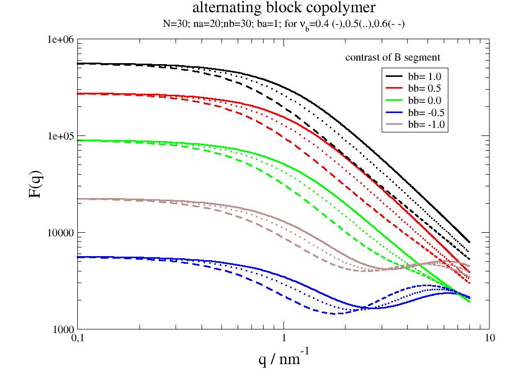
- jscatter.ff.alternatingCoPolymer(q, N, na, ba=1, nua=0.5, la=0.154, nb=None, lb=None, bb=None, nub=None)[source]
Alternating linear copolymer between collapsed and swollen states.
Single chain formfactor assuming alternating blocks of Gaussian coils between collapsed limit and swollen state in good solvent for dilute solutions. The formfactor reproduces diblock (equ 3.6 in [1]) and symmetric triblock copolymers for N=2,3.
- Parameters:
- qarray
Scattering vector in units 1/nm.
- Nint
Total number of blocks a,b with N=Na+Nb. For even N: Na=Nb otherwise Na=Nb+1.
- na,nbint
Number of segments/monomers in a block of type a or b.
- la,lbfloat
Segment/monomer length in nm. Default C-C bond length.
- nua,nubfloat
Excluded volume parameter nu describing chains between collapsed (1/3) and swollen states (3/5). nu =0.5 for a ideal chain or theta solvent condition.
- ba,bbfloat
Scattering length respective contrast to solvent of the segment/monomers . Might be calculated as from specific volume and scattering length \(ba = V_A (\rho_A-\rho_{solvent})\). For a melt the average scattering length is \(\rho = \frac{V_Ab_a + V_Bb_B}{V_A+V_B}\) leading to matching condition at low q. For a melt no interaction between chains.
- Returns:
- dataArray [q, Fq]
.I0 forward scattering q=0
Notes
We use equ 3.9 to 3.17 in [1] with explicit summation over blocks of type A and B with number Na and Nb.
\[ \begin{align}\begin{aligned}S(q) &= S_{AA}(q) + S_{BB}(q) + S_{AB}(q) + S_{BA}(q)\\S_{AA}(q) &= N_a S^{self}_{AA}(q) + S^{inter}_{AA}(q)\\S^{self}_{AA}(q) &= N_a F^2(\alpha_a,n_a,\nu_a)\\S^{inter}_{AA}(q) &= 2 n_a \sum_{k=1}^{N_a} (N_a-k) F^2(\alpha_a,n_a,\nu_a)E(\alpha_a,n_a,\nu_a)^{k-1}E(\alpha_a,n_a,\nu_a)^k\\S_{AB}(q) &= 2 n_a n_b \sum_{k=1}^{N_a-1} (N_a-k) F(\alpha_a,n_a,\nu_a)F(\alpha_b,n_b,\nu_b) E(\alpha_a,n_a,\nu_a)^{k-1}E(\alpha_b,n_b,\nu_b)^{k-1}\\S_{BA}(q) &= 2 n_a n_b \sum_{k=1}^{N_b} (N_b-k+1) F(\alpha_a,n_a,\nu_a)F(\alpha_b,n_b,\nu_b) E(\alpha_a,n_a,\nu_a)^{k-1}E(\alpha_b,n_b,\nu_b)^{k-1}\end{aligned}\end{align} \]with scattering variable \(\alpha=q^2l^2/6\) and
\[ \begin{align}\begin{aligned}E(\alpha,n,\nu) &= \sum_{i=1}^n e^{-\alpha(n-1)^{2\nu}}\\F(\alpha,n,\nu) &= \frac{1}{n} \sum_{i=1}^n e^{-\alpha(i-1)^{2\nu}} \; scattering \; amplitude\\P(\alpha,n,\nu) &= F^2(\alpha,n,\nu) \; formfactor\end{aligned}\end{align} \]- Notes:
A correction compared to [1] for \(S_{BA}\) is applied to get the correct forward scattering -> (Nb-k+1)
To normalize the formfactor use .I0 .
In the limit \(S(q \rightarrow \infty)\) the correlation terms should vanish and only the self terms \(S^{self}(q)\) should remain. Using the equations from [1] additional the terms \(S_{AB}(q)\) and \(S_{BA}(q)\) with k-1=0 adds. For conventional SAXS/SANS this difference is negligible.
References
Examples
Alternating blocks with different contrast and excluded volume parameter. The correlation peak between blocks is only visible for conditions close to matching of A and B segments, which also depends on block length.
import jscatter as js
import numpy as np
q=np.r_[0.1:8:0.02]

p=js.grace(1,1)
for i,nub in enumerate([0.4,0.5,0.6],1):
    for c,bb in zip([1,2,3,4,6],np.r_[1:-1.1:-0.5]):
        fq = js.ff.alternatingCoPolymer(q,N=30,na=20,nb=30,bb=bb,nub=nub)
        p.plot(fq.X,fq.Y,li=[i,2.5,c],sy=0,le=f'bb= {bb}' if i==1 else '')

p.yaxis(label='F(q)',scale='l',min=1000,max=1e6,charsize=1.5)
p.xaxis(scale='l',label='q / nm\S-1',charsize=1.5)
p.legend(x=3,y=5e5)
p.text('contrast of B segment',x=2,y=6e5)
p.title('alternating block copolymer')
p.subtitle(r'N=30; na=20;nb=30; ba=1; for \xn\f{}\sb\N=0.4 (-),0.5(..),0.6(- -)')
#p.save(js.examples.imagepath+'/alternatingCoPolymer.jpg')
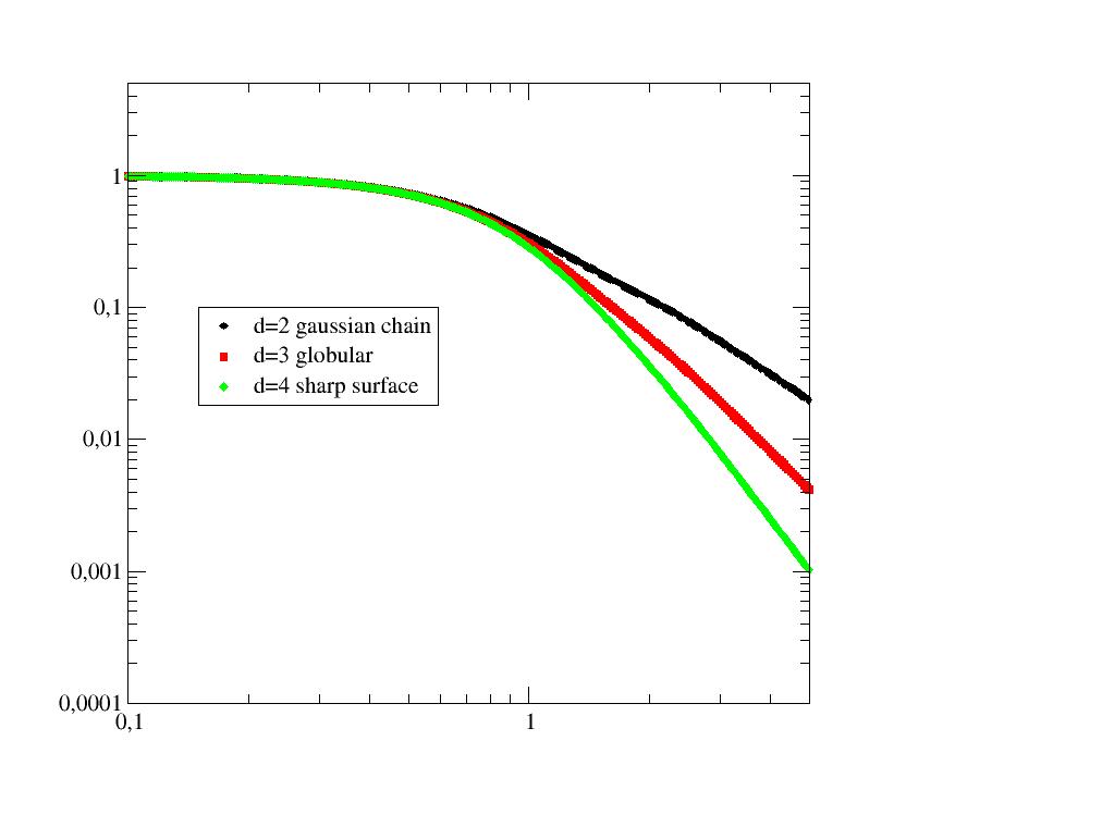
- jscatter.ff.beaucage(q, Rg=1, G=1, d=3)[source]
Beaucage introduced a model based on the polymer fractal model.
Beaucage used the numerical integration form (Benoit, 1957) although the analytical integral form was available [1]. This is an artificial connection of Guinier and Porod Regime . Better use the polymer fractal model [1] used in gaussianChain. For absolute scattering see introduction formfactor (ff).
- Parameters:
- qarray
Wavevector
- Rgfloat
Radius of gyration in 1/q units
- Gfloat
Guinier scaling factor, transition between Guinier and Porod
- dfloat
Power law exponent for large wavevectors
- Returns:
- dataArray
Columns [q,Fq]
Notes
Equation 9+10 in [1]
\[ \begin{align}\begin{aligned}I(q) &= G e^{-q^2 R_g^2 / 3.} + C q^{-d} \left[erf(qR_g / 6^{0.5})\right]^{3d}\\C &= \frac{G d}{R_g^d} \left[\frac{6d^2}{(2+d)(2+2d)}\right]^{d / 2.} \Gamma(d/2)\end{aligned}\end{align} \]with the Gamma function \(\Gamma(x)\) .
Various structures are related to the power law :
d = 5/3 fully swollen chains,
d = 2 ideal Gaussian chains and
d = 3 globular e.g. collapsed chains. (volume scattering)
d = 4 surface scattering at a sharp interface/surface (Porod scattering)
d = 6-dim rough surface area with a dimensionality dim between 2-3 (rough surface)
d < 3 mass fractals (eg gaussian chain dim = 2)
The Beaucage model is used to analyze small-angle scattering (SAS) data from fractal and particulate systems. It models the Guinier and Porod regions with a smooth transition between them and yields a radius of gyration and a Porod exponent. This model is an approximate form of an earlier polymer fractal model that has been generalized to cover a wider scope. The practice of allowing both the Guinier and the Porod scale factors to vary independently during nonlinear least-squares fits introduces undesired artefact’s in the fitting of SAS data to this model.
Examples
import jscatter as js
import numpy as np
q=js.loglist(0.1,5,300)
d2=js.ff.beaucage(q, Rg=2, d=2)
d3=js.ff.beaucage(q, Rg=2, d=3)
d4=js.ff.beaucage(q, Rg=2,d=4)
p=js.grace()
p.plot(d2,le='d=2 gaussian chain')
p.plot(d3,le='d=3 globular')
p.plot(d4,le='d=4 sharp surface')
p.yaxis(scale='l',min=1e-4,max=5)
p.xaxis(scale='l')
p.legend(x=0.15,y=0.1)
#p.save(js.examples.imagepath+'/beaucage.jpg')
 [1] (1,2,3)
Analysis of the Beaucage model Boualem Hammouda J. Appl. Cryst. (2010). 43, 1474–1478 http://dx.doi.org/10.1107/S0021889810033856
- jscatter.ff.cloudScattering(q, cloud, relError=50, formfactoramp=None, V=None, rms=0, ffpolydispersity=0, ncpu=0)[source]
Orientation averaged scattering of a cloud of isotropic particles.
Cloud can represent any object/lattice described by a cloud of scatterers with scattering amplitudes as constant, sphere scattering amplitude, Gaussian scattering amplitude or explicitly given one. The result is normalized by \(I_0=(\sum b_i)^2\) to equal one for q=0 (except for polydispersity).
.I0 represents the forward scattering.
Use \(b_i=b_vV_{unit cell}\) with \(b_v\) as scattering length density in the unit cell to get correct material scattering length density.
Remember that the atomic bond length are on the order 0.1-0.2 nm and crystal peaks are expected on this scale.
Methods to build clouds of scatterers e.g. a cube decorated with spheres at the corners can be found in Lattice with examples.
By default explicit spherical average is done. If rms and polydispersity are not needed the Debye-function can be used (for particle numbers<1000 it is faster).
- Parameters:
- qarray, ndim= Nx1
Radial wavevectors in 1/nm.
- cloudarray Nx3 or Nx4 or Nx5
Center positions cloud[:,:3] (in nm) of the N scatterers in the cloud.
If given cloud[:,3] is the scattering length \(b_i\) at positions cloud[:,:3], otherwise \(b=1\).
If given cloud[:,4] is the column index in formfactor for a specific scatterer.
To compare with material scattering length density \(b_v\) use \(b=b_vV_{unit cell}\) with \(b_v\) as scattering length density and \(V_{unit cell}\) as cloud unit cell volume.
- relErrorfloat
Determines calculation method.
relError>1 : Explicit calculation of spherical average with Fibonacci lattice on sphere of 2*relError+1 points. Already 150 gives good results (see Examples)
0<relError<1 : Monte Carlo integration on sphere until changes in successive iterations become smaller than relError. (Monte carlo integration with pseudo random numbers, see sphereAverage). This might take long for too small error.
relError=0 : The Debye equation is used (no asymmetry factor beta, no rms, no ffpolydispersity). Computation is of order \(N^2\) opposite to above which is order \(N\). For about 1000 particles same computing time,for 500 Debye is 4 times faster than above. If beta, rms or polydispersity is needed above.
- rmsfloat, default=0
Root mean square displacement \(\langle u^2 \rangle^{0.5}\) of the positions in cloud as random (Gaussian) displacements in nm.
Displacement u is randomly changed for each orientation in orientational average.
rms results in a Debye-Waller factor e.g. for crystal lattices and in diffuse scattering at high q.
Using a low number of displacements introduces noise on the model function because of bad sampling. To reduce this noise during fitting relError should be high (>2000 for linearPearls) and the result might be smoothed.
- formfactorampNone,’gauss’,’sphere’, array
Normalized scattering amplitudes of cloud points \(\hat{F_a^i}(q)\).
\(F_a(q)=b_i \hat{F_a^i}(q)\) with bi from cloud[3].
None : const scattering amplitude.
- ‘sphere’: Sphere scattering amplitude according to [3] equal for all cloud points.
Parameter V is needed to determine \(R\). The sphere radius is \(R=(\frac{3V}{4\pi})^{1/3}\)
- ‘gauss’Gaussian function \(\hat{F_a}(q) = exp(-\pi V^{2/3}q^2)\) according to [2]
Equal for all cloud points. The Gaussian shows no artificial minima compared to the sphere. Use parameter V to determine \(b_i\).
- ‘coil’Polymer coil (ideal Gaussian chain) showing scattering according to Debye function equal for all.
Parameter V needed to determine \(R_g = (\frac{3V}{4\pi})^{1/3}\). The scattering length is \(b_i = Nb_{monomer}\) with monomer number \(N\).
- Explicit isotropic \(\hat{F_a}(q)\) as array with [q,fa1(q),fa2(q),fa3(q),….].
If multiple fai are given the index i for a cloud point needs to be given in cloud[4]
The normalized scattering amplitude fa for each cloud point is calculated as fa=fai/fai[0]. Missing values are linear interpolated, q values outside interval are mapped to qmin or qmax.
Explicit formfactors are assumed to be isotropic.
If the scattering amplitude is not known \(F_a(q) \approx F^{1/2}(q)\) might be used as crude approximation for low Q.
- Vfloat, default=None
Volume of the scatterers to determine scattering amplitude (see formfactoramp). Only needed for formfactoramp ‘sphere’, ‘coil’ and ‘gauss’.
- ffpolydispersityfloat
Polydispersity of the gridpoints in relative units for sphere, gauss, explicit. Assuming F(q*R) for each gridpoint F is scaled as F(q*f*R) with f as normal distribution around 1 and standard deviation ffpolydispersity. The scattering length \(b\) is scaled according to the respective volume change by f**3. (f<0 is set to zero) assuming a volume scatterer. This results in a change of the forward scattering because of the stronger weight of larger objects.
- ncpuint, default 0
- Number of cpus used in the pool for multiprocessing.
not given or 0 : all cpus are used
int>0 : min(ncpu, mp.cpu_count)
int<0 : ncpu not to use
1 : single core usage for testing or comparing speed to Debye
- Returns:
- dataArray
- Columns [q, Pq, beta, fa]
Pq , formfactor , beta asymmetry factor, fa scattering amplitude
.I0 : \(=I(q=0)=(\sum_N b_i)^2\)
.sumblength : \(=\sum_N b_i\)
.formfactoramplitude : formfactor amplitude of cloudpoints according to type for all q values.
.formfactoramplitude_q : corresponding q values
Notes
We calculate the normalized formfactor \(\hat{F}(q)\) for \(N\) particles in a volume \(V\) after explicit orientational average \(<>\)
\[\hat{F}(q)=< \hat{F_a}(q) \cdot \hat{F_a}^*(q) >=< |\hat{F_a}(q)|^2 >\]with normalized scattering amplitude \(\hat{F_a}(q)\) and scattering length density \(b(r)\) (\(b_i(q)\) is the particle formfactor)
\[\hat{F_a}(q)= \int_V b(r) e^{i\mathbf{qr}} \mathrm{d}r / \int_V b(r) \mathrm{d}r = \sum_N b_i(q) e^{i\mathbf{qr}} / \sum_N b_i(0)\]The scattering intensity of a single object represented by the cloud is
\[I(q)=\hat{F}(q) \cdot (\int_V b(r) \mathrm{d}r)^2 = \hat{F}(q) \cdot (\sum_i b_i )^2\]beta is the asymmetry factor [1] \(beta =|< \hat{F_a}(q) >|^2 / < |\hat{F_a}(q)|^2 >\)
One has to expect a peak at \(q \approx 2\pi/d_{NN}\) with \(d_{NN}\) as the next neighbour distance between particles.
\(b_i(q)\) is a particle formfactor amplitude of the particles as e.g. q dependent Xray scattering amplitude or the formfactors in a cloud of different particles, but may also be constant as for neutron scattering atomic formfactors.
Random displacements \(u_i\) lead to \(r_i=r_i+u_i\) and to the Debye-Waller factor for Bragg peaks and diffusive scattering at higher q. See A nano cube build of different lattices .
The explicit orientational average can be simplified using the Debye scattering equation [4]
\[\hat{F}(Q)(\sum b_i)^2=\sum_i \sum_j b_i(q) b_j(q) \frac{\sin(qr_{ij})}{qr_{ij}} =\sum_i b_i(q)^2 + 2\sum_i \sum_{j>i} b_i(q) b_j(q) \frac{\sin(qr_{ij})}{qr_{ij}}\]Here no rms or ffpolydispersity are included. The calculation of \(beta\) requires an additional calculation.
The scattering of a cloud can represent the scattering of a cluster of particles with polydispersity and position distortion according to root-mean-square displacements (rms). Polydispersity and rms displacements are randomly changed within the orientational average to represent an ensemble average (opposite to the time average of a single cluster).
- Examples
See
latticeStructureFactor()for nanocubes.The model
linearPearls()uses cloudscattering. Look into the source code as example how to create a complex model.
References
[1]Kotlarchyk and S.-H. Chen, J. Chem. Phys. 79, 2461 (1983).1
[2]An improved method for calculating the contribution of solvent to the X-ray diffraction pattern of biological molecules Fraser R MacRae T Suzuki E IUCr Journal of Applied Crystallography 1978 vol: 11 (6) pp: 693-694
[3]X-ray diffuse scattering by proteins in solution. Consideration of solvent influence B. A. Fedorov, O. B. Ptitsyn and L. A. Voronin J. Appl. Cryst. (1974). 7, 181-186 doi: 10.1107/S0021889874009137
[4]Zerstreuung von Röntgenstrahlen Debye P. Annalen der Physik 1915 vol: 351 (6) pp: 809-823 DOI: 10.1002/andp.19153510606
Examples
The example compares to the analytic solution for an ellipsoid, then for a cube. For other shapes the grid may be better rotated away from the object symmetry or a random grid should be used. The example shows a good approximation with NN=20. Because of the grid peak at \(q=2\pi/d_{NN}\) the grid scatterer distance \(d_{NN}\) should be \(d_{NN} < \frac{1}{3} 2\pi/q_{max}\) .
Inspecting A nano cube build of different lattices shows other possibilities building a grid. Also, a pseudo random grid can be used
pseudoRandomLattice().# ellipsoid with grid build by mgrid import jscatter as js import numpy as np import matplotlib.pyplot as plt from mpl_toolkits.mplot3d import Axes3D # cubic grid points R=3;NN=20;relError=50 grid= np.mgrid[-R:R:1j*NN, -R:R:1j*NN,-2*R:2*R:2j*NN].reshape(3,-1).T # points inside of sphere with radius R p=1;p2=1*2 # p defines a superball with 1->sphere p=inf cuboid .... inside=lambda xyz,R1,R2,R3:(np.abs(xyz[:,0])/R1)**p2+(np.abs(xyz[:,1])/R2)**p2+(np.abs(xyz[:,2])/R3)**p2<=1 insidegrid=grid[inside(grid,R,R,2*R)] q=np.r_[0:5:0.1] p=js.grace() p.title('compare form factors of an ellipsoid') ffe=js.ff.cloudScattering(q,insidegrid,relError=relError) p.plot(ffe,legend='cloud ff explicit') ffa=js.ff.ellipsoid(q,2*R,R) p.plot(ffa.X,ffa.Y/ffa.I0,li=1,sy=0,legend='analytic formula') p.yaxis(scale='log') p.legend(x=2,y=0.1) # show only each 10th point js.mpl.scatter3d(insidegrid[::10,:])
# cube
# grid points generated by cubic grid
import jscatter as js
import numpy as np

q=np.r_[0.1:5:0.1]
p=js.grace()
R=3;N=10;relError=0.01  # random points on sphere
grid= js.sf.scLattice(R/N,N)

ffe=js.ff.cloudScattering(q,grid,relError=relError)
p.plot(ffe,legend='cloud ff explicit 10')
# each point has a cube around it including the border
ffa=js.ff.cuboid(q,2*R+R/N)
p.plot(ffa.X,ffa.Y/ffa.I0,li=1,sy=0,legend='analytic formula')

p.yaxis(scale='l')
p.title('compare form factors of a cube')
p.legend(x=2,y=0.1)
An objekt with explicit given formfactoramp for each gridpoint.
import jscatter as js
import numpy as np
q = js.loglist(0.01, 7, 100)
# 5 coreshell particles in line with polydispersity
rod0 = np.zeros([5, 3])
rod0[:, 1] = np.r_[0, 1, 2, 3, 4] * 4
cs = js.ff.sphereCoreShell(q=q, Rc=1, Rs=2, bc=0.1, bs=1, solventSLD=0)
csa = np.c_[cs.X,cs[2]].T
ffe = js.ff.cloudScattering(q, rod0, formfactoramp=csa,relError=100,ffpolydispersity=0.1)
p=js.grace()
p.plot(ffe)
Using cloudScattering as fit model.
We have to define a model that parametrizes the building of the cloud that we get fit parameters. As example, we use two overlapping spheres. The model can be used to fit some data. The build of the model is important as it describes how the overlap is treated e.g. as average.
- We have to consider some points:
It is important that the model is continuous in its parameters to avoid steps as any fit algorithm cannot handle this.
We have to limit some parameters that make giant grids. Fit algorithm make first a small step then a large one to estimate a good step size for parameter changes. If in the dumbbell example the radii R1 or R2 is increased to >1000 then the grid size burst the RAM and we get a Memory Error. Use hard limits for the radii to a reasonable value as shown below (see setlimit).
The argument “diff_step” increases the initial step size as x*diff_step, which is in default something like machine epsilon (~1e-8, so just small). Change it to 0.01 to jump over local minima and find an improved fit.
In the below example the first fit is fast but bad as we find a local minimum.
diff_step=0.01imroves this dramatically and is still fast A global fit algorithm takes quite long but finds the correct solution.
import jscatter as js
import numpy as np
#
#: test if distance from point on X axis
isInside=lambda x,A,R:((x-np.r_[A,0,0])**2).sum(axis=1)**0.5<R
#: model
def dumbbell(q,A,R1,b1,bgr=0,dx=0.3,relError=50):
    # D sphere distance
    # R1, R2 radii
    # b1,b2  scattering length
    # bgr background
    # dx grid distance not a fit parameter!!
    R2=R1
    b2=b1
    mR=max(R1,R2)

    # xyz coordinates
    grid=np.mgrid[-A/2-mR:A/2+mR:dx,-mR:mR:dx,-mR:mR:dx].reshape(3,-1).T
    insidegrid=grid[isInside(grid,-A/2.,R1) | isInside(grid,A/2.,R2)]

    # add blength column
    insidegrid=np.c_[insidegrid,insidegrid[:,0]*0]

    # set the corresponding blength; the order is important as here b2 overwrites b1
    insidegrid[isInside(insidegrid[:,:3],-A/2.,R1),3]=b1
    insidegrid[isInside(insidegrid[:,:3],A/2.,R2),3]=b2

    # and maybe a mix ; this depends on your model
    insidegrid[isInside(insidegrid[:,:3],-A/2.,R1) & isInside(insidegrid[:,:3],A/2.,R2),3]=(b2+b1)/2.

    # calc the scattering
    result=js.ff.cloudScattering(q,insidegrid,relError=relError)
    result.Y=result.Y*result.I0+bgr

    # add attributes for later usage
    result.A=A
    result.R1=R1
    result.b1=b1
    result.dx=dx
    result.insidegrid=insidegrid
    return result
#
# test it
q=np.r_[0.01:5:0.02]
data=dumbbell(q,3,2,1)

# show result configuration
js.mpl.scatter3d(data.insidegrid[:,0],data.insidegrid[:,1],data.insidegrid[:,2])
#
# Fit your data like this.
# It may be a good idea to use not the highest resolution in the beginning because of speed.
# If you have a good set of starting parameters you can decrease dx.
data2=data.prune(number=100)
data2.makeErrPlot(yscale='l')

data2=data.prune(number=100)
data2.makeErrPlot(yscale='l')
data2.setLimit(R1=[None,None,1,4],A=[None,None,1,10])

# this results in a fast but bad fit result
# a local minima is found but the basics is working.
# Using diff_step=0.01 finds a good solution
data2.fit(model=dumbbell,
           freepar={'A':3,'R1':2.4,'b1':1},
           fixpar={'dx':0.3,'bgr':0},
           mapNames={'q':'X'},diff_step=None)

if 0:
    # To get a good result we need to find the global minimum by a different algorithm ('differential evolution')
    # The limits are used as border to search in a limited area.
    # The fit takes about 3500 iterations (1000s on Ryzen 1600X 6 cores)
    data2.fit(model=dumbbell,method='differential_evolution',
               freepar={'A':3,'R1':2.4,'b1':1},
               fixpar={'dx':0.3,'bgr':0},
               mapNames={'q':'X'})
Fit a sphere formfactoramp.
The quality of the grid approximation (number of gridpoints) may improve the correct description of higher order minima.
import numpy as np
import jscatter as js

# a function to discriminate what is inside of the sphere
# basically a superball p2=2 is a sphere
inside=lambda xyz,R1,p2:(np.abs(xyz[:,0]))**p2+(np.abs(xyz[:,1]))**p2+(np.abs(xyz[:,2]))**p2<=R1**2

def test(q,R,b,p2=2,relError=20):
    # make cubic grid with right size (increase NN for better approximation)
    NN=20
    grid= np.mgrid[-R:R:1j*NN, -R:R:1j*NN,-R:R:1j*NN].reshape(3,-1).T
    # cut the edges to get a sphere
    insidegrid=grid[inside(grid,R,p2)]
    # add scattering length for points
    # the average scattering length density is sum(b)/sphereVolume
    insidegrid=np.c_[insidegrid,insidegrid[:,0]*0]
    insidegrid[:,3]=b
    # calc formfactor (normalized) for a single sphere
    ffs=js.ff.cloudScattering(q,insidegrid,relError=relError)
    # the total scattering is sumblength**2
    ffs.Y*=ffs.sumblength**2
    # save radius and the grid for later
    ffs.R=R
    ffs.insidegrid=insidegrid
    return ffs

####main
q=np.r_[0:3:0.01]
sp=js.formfactor.sphere(q,3,1)

sp.makeErrPlot(yscale='l')   # show intermediate results
sp.setlimit(R=[0.3,10])      # set some reasonable limits for R
sp.fit(model=test,
    freepar={'b':6,'R':2.1},
    fixpar={},
    mapNames={'q':'X'})

# show the resulting sphere grid
resultgrid=sp.lastfit.insidegrid
js.mpl.scatter3d(resultgrid[:,0],resultgrid[:,1],resultgrid[:,2])
Here we compare explicit calculation with the Debye equation as the later gets quite slow for larger numbers.
import jscatter as js
import numpy as np
R=6;NN=20
q=np.r_[0:5:0.1]
grid=js.formel.randomPointsInCube(10000)*R-R/2
ffe=js.ff.cloudScattering(q,grid,relError=150)    # takes about  1.3 s on six core
ffd=js.ff.cloudScattering(q,grid,relError=0)      # takes about 11.4 s on six core
grid=js.formel.randomPointsInCube(500)*R-R/2
ffe=js.ff.cloudScattering(q,grid,relError=150)    # takes about 132 ms on six core
ffd=js.ff.cloudScattering(q,grid,relError=0)      # takes about  33 ms on six core

p=js.grace()
p.plot(ffe)
p.plot(ffd)
p.yaxis(scale='l')
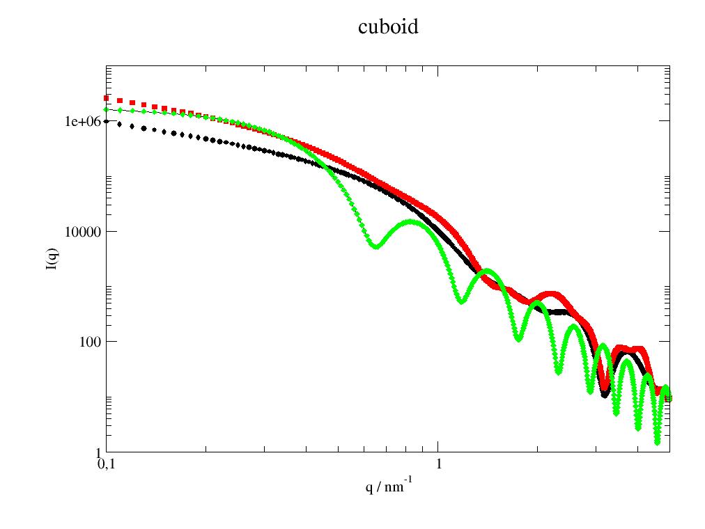
- jscatter.ff.cuboid(q, a, b=None, c=None, SLD=1, solventSLD=0, N=30)[source]
Formfactor of rectangular cuboid with different edge lengths.
- Parameters:
- qarray
Wavevector in 1/nm
- a,b,cfloat, None
Edge length, for a=b=c its a cube, Units in nm. If b=None b=a. If c=None c=b.
- SLDfloat, default =1
Scattering length density of cuboid.unit nm^-2 e.g. SiO2 = 4.186*1e-6 A^-2 = 4.186*1e-4 nm^-2 for neutrons
- solventSLDfloat, default =0
Scattering length density of solvent. unit nm^-2 e.g. D2O = 6.335*1e-6 A^-2 = 6.335*1e-4 nm^-2 for neutrons
- Nint
Order for Gaussian integration over both phi and theta.
- Returns:
- dataArray
- Columns [q,Iq]
.I0 forward scattering
.edges
.contrast
Notes
\[I(q)=\rho^2V_{cube}^2 \int_{0}^{2\pi}\int_{0}^{\pi} \lvert sinc(q_xa/2 ) sinc(q_yb/2) sinc(q_zc/2)\rvert^2 \sin\theta d\theta d\phi\]with \(q = (q_x,q_y,q_z) = (q\sin\theta\cos\phi,q\sin\theta\sin\phi,q\cos\theta)\) and contrast \(\rho\) [1].
In [1] the edge length is only half of it.
References
[1] (1,2)Analysis of small-angle scattering data from colloids and polymer solutions: modeling and least-squares fitting Pedersen, Jan Skov Advances in Colloid and Interface Science 70, 171 (1997) http://dx.doi.org/10.1016/S0001-8686(97)00312-6
Examples
import jscatter as js
import numpy as np
q=np.r_[0.1:5:0.01]
p=js.grace()
p.plot(js.ff.cuboid(q,60,4,6))
p.plot(js.ff.cuboid(q,10,4,60))
p.plot(js.ff.cuboid(q,11,11,11),li=1)
p.yaxis(scale='l',label='I(q)')
p.xaxis(scale='l',label='q / nm\S-1')
p.title('cuboid')
#p.save(js.examples.imagepath+'/cuboid.jpg')
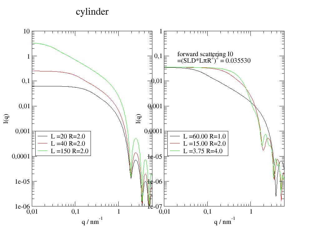
- jscatter.ff.cylinder(q, L, radius, SLD=0.001, solventSLD=0, alpha=None, nalpha=90, h=None)[source]
Cylinder form factor including cap.
Based on multiShellCylinder (see there for detailed description of parameters).
- Parameters:
- qarray
Scattering vector i units 1/nm.
- Lfloat
Length in nm.
- radiusfloat
Radius in nm.
- hfloat
Cap geometry
- SLDfloat
Cylinder scattering length density in units nm^-2.
- solventSLDfloat
Solvent scattering length density in units nm^-2.
- hfloat, default=None
Geometry of the cap with radii R=(r**2+h**2)**0.5 in units nm. h is distance of cap center with radius R from the flat cylinder cap and r as radius of the cylinder.
None No cap, flat end as default.
0 cap radius equal cylinder radius
>0 cap radius larger cylinder radius as barbell
<0 cap radius smaller cylinder radius as lens cap
- alphafloat, [float,float] , default [0,pi/2], unit rad
Orientation, angle between the cylinder axis and the scattering vector q in units rad. 0 means parallel, pi/2 is perpendicular If alpha =[start,end] is integrated between start,end start > 0, end < pi/2
- nalphaint, default 90
Number of points in Gauss integration along alpha.
Notes
Compared to SASview (5.0) this yields a factor 2 less intensity. Correctness can be checked as the forward scattering .I0 is independent of orientation and should be equal V² (V is volume) if SLD=1 and solvent SLD=0.
Definition of parameters can be seen in this figure ignoring the outer shell. See
multiShellCylinder():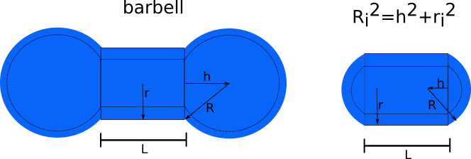
References
[1]Guinier, A. and G. Fournet, “Small-Angle Scattering of X-Rays”, John Wiley and Sons, New York, (1955)
Examples
The typical long cylinder formfactor with a linear region for long cylinders.
import jscatter as js
import numpy as np
q=js.loglist(0.01,8,500)
p=js.grace()
p.multi(1,2)
R=2
for L in [20,40,150]:
    cc=js.ff.cylinder(q,L=L,radius=R)
    p[0].plot(cc,li=-1,sy=0,le='L ={0:.0f} R={1:.1f}'.format(L,R))
L=60
for R in [1,2,4]:
    cc=js.ff.cylinder(q,L=L/R**2,radius=R)
    p[1].plot(cc,li=-1,sy=0,le='L ={0:.2f} R={1:.1f}'.format(L/R**2,R))
p[0].yaxis(label='I(q)',scale='l',min=1e-6,max=10)
p[0].xaxis(label='q / nm\S-1',scale='l',min=0.01,max=6)
p[1].yaxis(label='I(q)',scale='l',min=1e-7,max=1)
p[1].xaxis(label='q / nm\S-1',scale='l',min=0.01,max=6)
p[1].text(r'forward scattering I0\n=(SLD*L\xp\f{}R\S2\N)\S2\N = 0.035530',x=0.02,y=0.1)
p.title('cylinder')
p[0].legend(x=0.012,y=0.001)
p[1].legend(x=0.012,y=0.0001)
#p.save(js.examples.imagepath+'/cylinder.jpg')
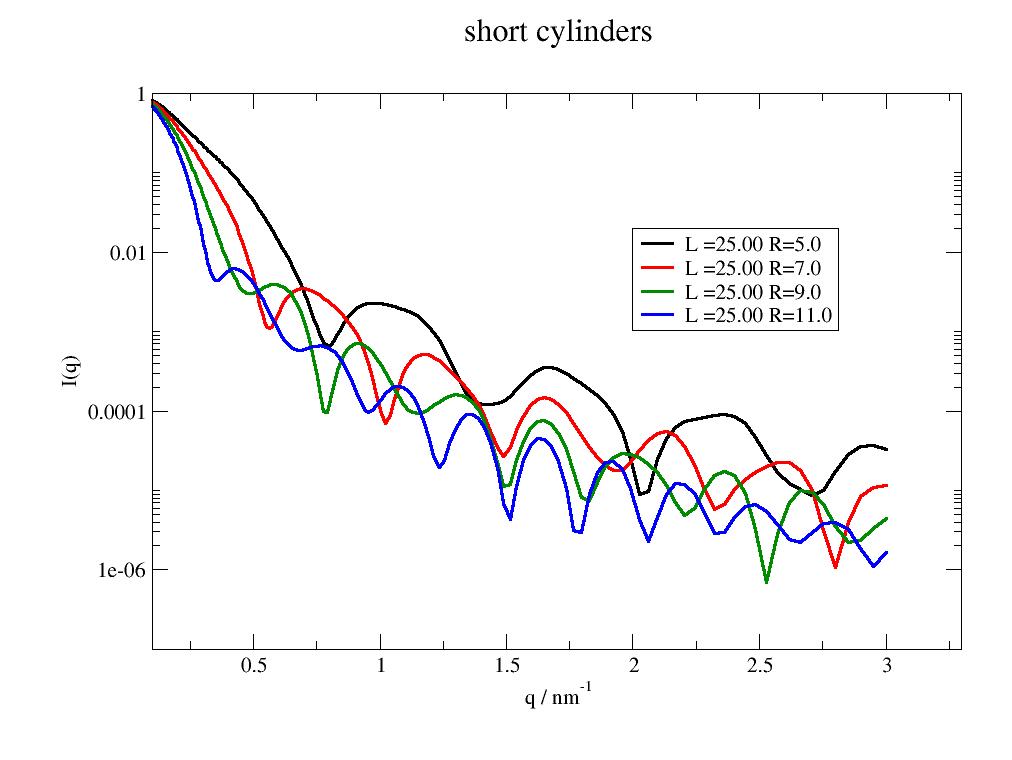
The following short cylinders highlight the peak shape which can differ from expectations. Dependent on R, L interferences we see flattened peaks and that consecutive peaks also differ in shape.
import jscatter as js
import numpy as np
q=js.loglist(0.1,3,200)
p=js.grace()
L=25
for R in np.r_[5:12:2]:
    cc=js.ff.cylinder(q,L=L,radius=R)
    p.plot(cc.X,cc.Y/cc.I0,li=[1,3,-1],sy=0,le='L ={0:.2f} R={1:.1f}'.format(L,R))
p.yaxis(label='I(q)',scale='l')
p.xaxis(label='q / nm\S-1',scale='n',min=0.1,max=3.3)
p.title('short cylinders')
p.legend(x=2,y=0.02)
#p.save(js.examples.imagepath+'/cylindershort.jpg')
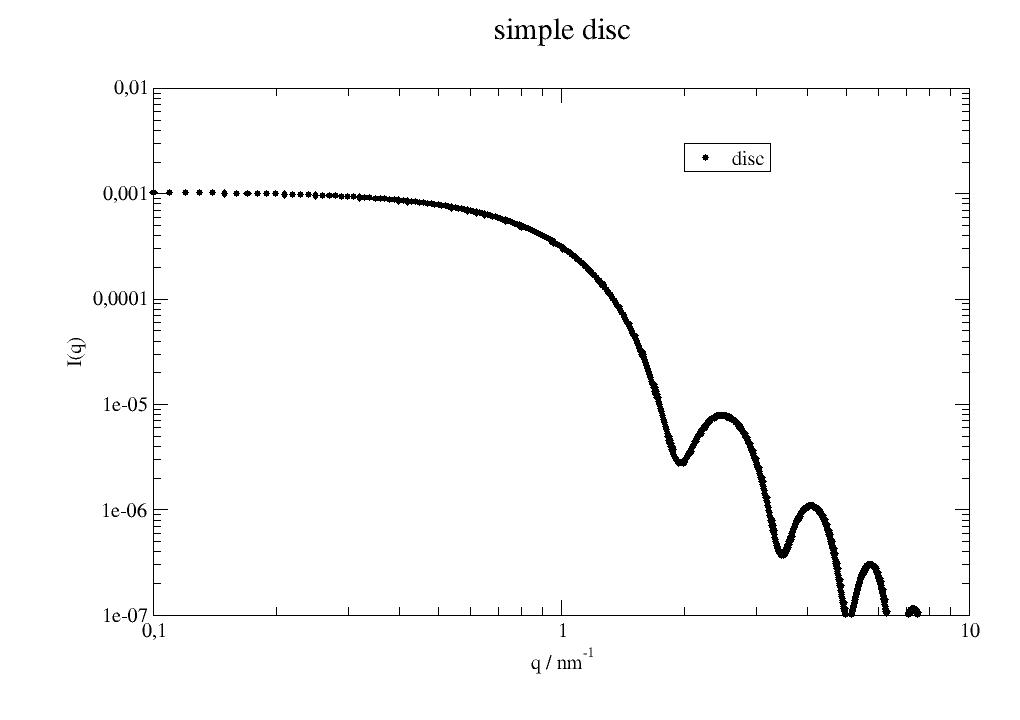
- jscatter.ff.disc(q, R, D, SLD, solventSLD=0, alpha=None)[source]
Disc form factor .
- Parameters:
- qarray
Wavevectors, units 1/nm
- Rfloat
Radius in nm.
- Dfloat
Thickness of the disc in units nm.
- SLD,solventSLDfloat
Scattering length density in nm^-2.
- alphafloat, [float,float] , unit rad
Orientation, angle between the cylinder axis and the scattering vector q. 0 means parallel, pi/2 is perpendicular If alpha =[start,end] is integrated between start,end start > 0, end < pi/2
Notes
For details see
multiShellDisc().Examples
Simple disc. The short high Q modulation is caused by the radius interference. A radial distribution might be needed for thin discs.
import jscatter as js
import numpy as np
x=np.r_[0.01:5:0.01]
p=js.grace()

# single disc
bshell = js.ff.disc(x,10,3.5,6.39e-4)
p[0].plot(bshell, le='disc')

p[0].yaxis(label='I(q)',scale='l',min=1e-7,max=1)
p[0].xaxis(label='q / nm\S-1',scale='l',min=0.1,max=10)
p[0].legend(x=2,y=0.003)
p[0].title('simple disc')
# p.save(js.examples.imagepath+'/simpleDisc.jpg')
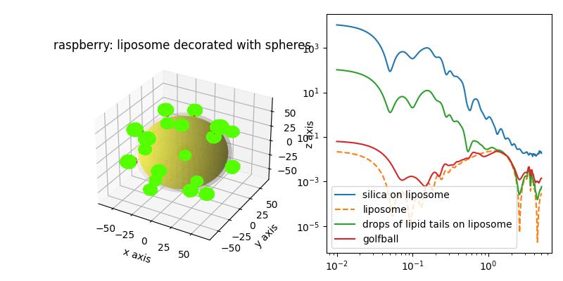
- jscatter.ff.dropDecoratedCoreShell(q, Rcore, Rdrop, Ndrop, Hdrop, coreSLD, dropSLD, shellthickness=None, shellSLD=None, solventSLD=0, typ='drop', distribution='fibonacci', dR=0.2, dRdrop=0.1, ndrop=5, relError=100, cmap='hsv', show=False)[source]
A multi shell particle decorated with droplets.
- The model described a core shell particle decorated with drops.
Drops may be added only at the outer surface extending the volume or extending into the inner volume.
Using a zero shellthickness drops decorate a sphere like the raspberry model for pickering emulsions.
Drops with solventSLD make a golfball like surface with spher section cuts.
- Parameters:
- qarray
Wavevectors in units 1/nm.
- Rcorefloat
Core radius in nm.
- shellthicknessfloat or list of float
Thickness of consecutive shells from core to outside in units nm. Might be zero.
- shellSLDfloat or list of float
Scattering length of consecutive shells corresponding to shellthickness. Unit is nm^-2
- dropSLDfloat or list of float
Scattering length of drop in unit nm^-2. For typ=’disc’ a list corresponding to shellSLD for each shell. For other typ a float as drop has a constant SLD.
- Rdropfloat,
Radius of small drops or discs decorating the shell in units nm.
- dRdropfloat,
Relative polydispersity of drop radius.
- Ndropint
Number of drops on shell.
- Hdropfloat
Center of drops relative to outside_radius = Rcore+sum(shellthickness).
- coreSLDfloat
Scattering length of core in unit nm^-2.
- solventSLDfloat
Solvent scattering length density in unit nm^-2.
- typ‘cutdrop’, default ‘drop’
- Type of the drops
‘drop’ drops extending to inside and outside, drop volume has SLD dropSLD. Like particles penetrating the shells.
- ‘cutdrop’ the drop is outside and cut at the outer shell.
The shell itself is not modified as Particles attached to the surface.
- distribution‘fibonacci’,’quasirandom’
- Distribution of drops as :
- ‘fibonacci’ A Fibonacci lattice (near hexagonal) on the sphere with Ndrop points.
For even Ndrop the point [0,0,1] is removed.
‘quasirandom’ quasirandom distribution of Ndrop drops on sphere surface.
The distributions are always the same if repeated several times.
- dRfloat, default 0.1
Fluctuation of Rcore (or shellthickness[0] if rcore=0). This radius polydispersity suppresses the strong minima of a multishell structure at high q and reduce there depth at low Q to get a more realistic pattern. Drops are scaled along the drop center to keep relative position to shells. The size is not changed.
- ndropint
Number of points in grid on length sum(shellthickness). Determines resolution of the droplets. Large ndrop increase the calculation time by ndrop**3. To small give wrong scattering length contributions in shell and core.
- relErrorfloat
Determines calculation method. See
cloudScattering()- showbool
Show a 3D image using matplotlib.
- cmapmatplotlib colormap name
Only for show to determine the colormap. See js.mpl.showColors() for all possibilities.
- Returns:
- dataArray
- Columns [q, Fq, Fq coreshell]
attributes from call
.dropSurfaceFraction \(=N_{drop}R_{drop}^2/(4(R_{core} + shellthickness + H_{drop})^2)\)
Notes
- The models uses cloudscattering with multi component particle distribution.
At the center is a multiShellSphere with core and shell located.
At the positions of droplets a grid of small particles describe the respective shape as disc or drop.
According to the ‘typ’ each particle gets a respective scattering length to result in the correct scattering length density including the overlap with the central core-shell particle.
cloudscattering is used to calculate the respective scattering including all cross terms.
If drops overlap the overlap volume is only counted once. For large Ndrop the drop layer might be full, check .dropSurfaceFraction. In this case the disc represents the shell, while the drops represent still some surface roughness. The Rdrop is explicitly not limited to allow this.
As described in cloudscattering for high q a bragg peak will appear showing the particle bragg peaks. This is far outside the respective SAS scattering. The validity of this model is comparable to A nano cube build of different lattices. For higher q the ndrop resolution parameter needs to be increased.
References
[1]Softening of phospholipid membranes by the adhesion of silica nanoparticles – as seen by neutron spin-echo (NSE) Ingo Hoffmann et al Nanoscale, 2014, 6, 6945-6952 ; https://doi.org/10.1039/C4NR00774C
Examples
Liposome decorated with particles Silica particles on a liosome were examined in[1]. The multiCoreShell of the liposome is decorated with 8 nm silica nanoparticles. We may use a particle with less contrast or with solvent SLD to generate a golfball like object or a layer with holes.
The glfball shows increased scattering as the multilayer matching condition is changed.
The liposme core shell shows the reduced low Q scattering as the head and tail regions in SAXs nearly match each other. Accordingly, the silica partiles dominate the low Q scattering. We observe a drop structure factor in midrange Q.and additional minima from the silica sphere formfactor.
import jscatter as js
import numpy as np
q=js.loglist(0.01,5,300)

# thickness of head and tail region of lipid bilayer
st = [0.75,2.8,0.75]
# corresponding contrast
fe = js.formel.felectron
sSLD = 335 * fe  # H2O unit e/nm³*fe
sld = np.r_[420* fe,290* fe,420* fe]  # unit e/nm³*fe
dSLD = 796 * fe # Silica unit e/nm³*fe
R = 8
dR = 3  # size polydispersity

fig = js.ff.dropDecoratedCoreShell(q=q,Rcore=50, Rdrop=R, Ndrop=20, Hdrop=R, dR=dR, cmap='prism',
                coreSLD=sSLD, shellthickness=st, shellSLD=sld, dropSLD=dSLD, solventSLD=sSLD, show=1, typ='drop')

bb=fig.axes[0].get_position()
fig.axes[0].set_title('raspberry: liposome decorated with spheres')
fig.axes[0].set_position(bb.shrunk(0.5,0.9))
ax1=fig.add_axes([0.58,0.1,0.4,0.85])

silica = js.ff.dropDecoratedCoreShell(q=q,Rcore=50, Rdrop=R, Ndrop=20, Hdrop=R ,dR=dR,ndrop=7,
                coreSLD=sSLD, shellthickness=st, shellSLD=sld, dropSLD=dSLD, solventSLD=sSLD, show=0, typ='drop')
ax1.plot(silica.X,silica.Y, label='silica on liposome')
ax1.plot(silica.X,silica._cs_fq,linestyle='--', label='liposome')

# less contrast than the silica , same as inside bilayer
drop = js.ff.dropDecoratedCoreShell(q=q,Rcore=50, Rdrop=R, Ndrop=20, Hdrop=R ,dR=dR,ndrop=7,
                coreSLD=sSLD, shellthickness=st, shellSLD=sld, dropSLD=sld[1], solventSLD=sSLD, show=0, typ='drop')
ax1.plot(drop.X,drop.Y, label='drops of lipid tails on liposome')

# drops with solvent SLD cut spheres from the liposome
golfball = js.ff.dropDecoratedCoreShell(q=q,Rcore=50, Rdrop=R, Ndrop=40, Hdrop=R-sum(st) ,dR=dR, ndrop=7,dRdrop=0,
                coreSLD=sSLD, shellthickness=st, shellSLD=sld, dropSLD=sSLD, solventSLD=sSLD, show=0, typ='drop')
ax1.plot(golfball.X,golfball.Y, label='golfball')

ax1.set_yscale('log')
ax1.set_xscale('log')
ax1.legend()
fig.set_size_inches(8,4)
# fig.savefig(js.examples.imagepath+'/raspberry.jpg')
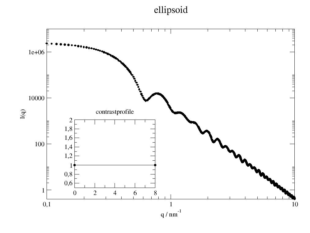
- jscatter.ff.ellipsoid(q, Ra, Rb, SLD=1, solventSLD=0, alpha=None, tol=1e-06)[source]
Form factor for a simple ellipsoid (ellipsoid of revolution).
- Parameters:
- qfloat
Scattering vector unit e.g. 1/A or 1/nm 1/Ra
- Rafloat
Radius rotation axis units in 1/unit(q)
- Rbfloat
Radius rotated axis units in 1/unit(q)
- SLDfloat, default =1
Scattering length density of unit nm^-2 e.g. SiO2 = 4.186*1e-6 A^-2 = 4.186*1e-4 nm^-2 for neutrons
- solventSLDfloat, default =0
Scattering length density of solvent. unit nm^-2 e.g. D2O = 6.335*1e-6 A^-2 = 6.335*1e-4 nm^-2 for neutrons
- alpha[float,float] , default [0,90]
Angle between rotation axis Ra and scattering vector q in unit grad Between these angles orientation is averaged alpha=0 axis and q are parallel, other orientation is averaged
- tolfloat
relative tolerance for integration between alpha
- Returns:
- dataArray
- Columns [q; Iq; beta ]
.RotationAxisRadius
.RotatedAxisRadius
.EllipsoidVolume
.I0 forward scattering q=0
beta is asymmetry factor according to [3]. \(\beta = |<F(Q)>|^2/<|F(Q)|^2>\) with scattering amplitude \(F(Q)\) and form factor \(P(Q)=<|F(Q)|^2>\)
Notes
See
triaxialEllipsoid()with Rb=Rc for the equation.References
[1]Structure Analysis by Small-Angle X-Ray and Neutron Scattering Feigin, L. A, and D. I. Svergun, Plenum Press, New York, (1987).
[3]Kotlarchyk and S.-H. Chen, J. Chem. Phys. 79, 2461 (1983).
Examples
Simple ellipsoid in vacuum:
import jscatter as js
import numpy as np
x=np.r_[0.1:10:0.01]
Rp=6.
Re=8.
elli = js.ff.ellipsoid(x,Rp,Re,1)
# plot it
p=js.grace()
p.plot(elli)
p.yaxis(scale='l',label='I(q)',min=0.01,max=100)
p.xaxis(scale='l',label='q / nm\S-1',min=0.1,max=10)
p.title('ellipsoid')
# p.save(js.examples.imagepath+'/ellipsoid.jpg')
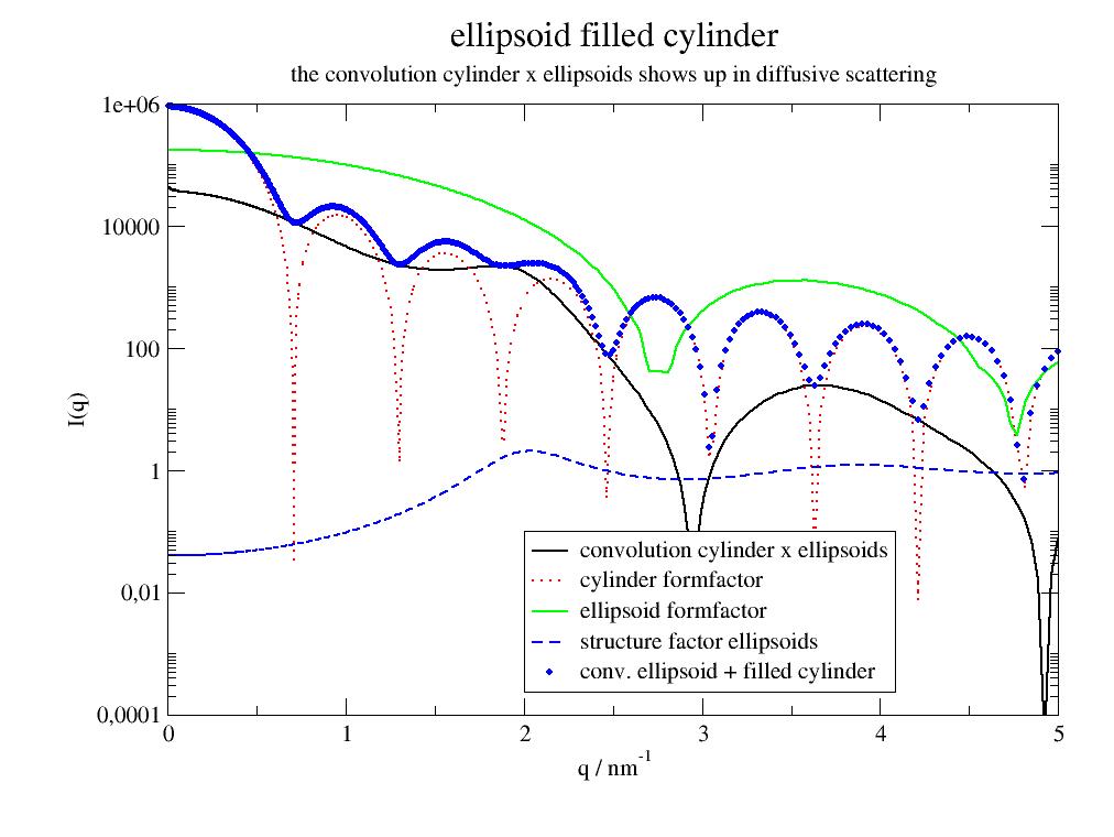
- jscatter.ff.ellipsoidFilledCylinder(q=1, R=10, L=0, Ra=1, Rb=2, eta=0.1, SLDcylinder=0.1, SLDellipsoid=1, SLDmatrix=0, alpha=90, epsilon=None, fPY=1, dim=3)[source]
Scattering of a single cylinder filled with ellipsoidal particles .
A cylinder filled with ellipsoids of revolution with cylinder formfactor and ellipsoid scattering as described by Siefker [1]. Ellipsoids have a fluid like distribution and hard core interaction leading to Percus-Yevick structure factor between ellipsoids. Ellipsoids can be oriented along cylinder axis. If cylinders are in a lattice, the ellipsoid scattering (column 2) is observed in the diffusive scattering and the dominating cylinder contributes only to the bragg peaks as a form factor.
- Parameters:
- qarray
Wavevectors in units 1/nm
- Rfloat
Cylinder radius in nm
- Lfloat
Length of the cylinder in nm If zero infinite length is assumed, but absolute intensity is not valid, only relative intensity.
- Rafloat
Radius rotation axis units in nm
- Rbfloat
Radius rotated axis units in nm
- etafloat
Volume fraction of ellipsoids in cylinder for use in Percus-Yevick structure factor. Radius in PY corresponds to sphere with same Volume as the ellipsoid.
- SLDcylinderfloat,default 1
Scattering length density cylinder material in nm**-2
- SLDellipsoidfloat,default 1
Scattering length density of ellipsoids in cylinder in nm**-2
- SLDmatrixfloat
Scattering length density of the matrix outside the cylinder in nm**-2
- alphafloat, default 90
Orientation of the cylinder axis to wavevector in degrees
- epsilon[float,float], default [0,90]
Orientation range of ellipsoids rotation axis relative to cylinder axis in degrees.
- fPYfloat
Factor between radius of ellipsoids Rv (equivalent volume) and radius used in structure factor Rpy Rpy=fPY*(Ra*Rb*Rb)**(1/3)
- dim3,1, default 3
Dimensionality of the Percus-Yevick structure factor 1 is one dimensional stricture factor, anything else is 3 dimensional (normal PY)
- Returns:
- dataArray
- Columns [q,n*conv(ellipsoids,cylinder)*sf_b + cylinder,
n *conv(ellipsoids,cylinder)*sf_b, cylinder, n * ellipsoids, sf, beta_ellipsoids]
Each contributing formfactor is given with its absolute contribution \(V^2contrast^2\) (NOT normalized to 1)
The observed structurefactor is \(sf\_b = S_{\beta}(q)=1+\beta (S(q)-1)\).
beta_ellipsoids \(=\beta(q)\) is the asymmetry factor of Kotlarchyk and Chen [2].
conv(ellipsoids,cylinder) -> ellipsoid formfactor convoluted with cylinder formfactor
.ellipsoidNumberDensity -> n ellipsoid number density in cylinder volume
.cylinderRadius
.cylinderLength
.cylinderVolume
.ellipsoidRa
.ellipsoidRb
.ellipsoidRg
.ellipsoidVolume
.ellipsoidVolumefraction
.ellipsoidNumberDensity unit 1/nm**3
.alpha orientation range
.ellipsoidAxisOrientation
References
[1]Confinement Facilitated Protein Stabilization As Investigated by Small-Angle Neutron Scattering. Siefker, J., Biehl, R., Kruteva, M., Feoktystov, A., & Coppens, M. O. (2018) Journal of the American Chemical Society, 140(40), 12720–12723. https://doi.org/10.1021/jacs.8b08454
[2]Kotlarchyk and S.-H. Chen, J. Chem. Phys. 79, 2461 (1983).
Examples
import jscatter as js
p=js.grace()
q=js.loglist(0.01,5,800)
ff=js.ff.ellipsoidFilledCylinder(q,L=100,R=5.4,Ra=1.63,Rb=1.63,eta=0.4,alpha=90,epsilon=[0,90],SLDellipsoid=8)
p.plot(ff.X,ff[2],li=[1,2,-1],sy=0,legend='convolution cylinder x ellipsoids')
p.plot(ff.X,ff[3],li=[2,2,-1],sy=0,legend='cylinder formfactor')
p.plot(ff.X,ff[4],li=[1,2,-1],sy=0,legend='ellipsoid formfactor')
p.plot(ff.X,ff[5],li=[3,2,-1],sy=0,legend='structure factor ellipsoids')
p.plot(ff.X,ff.Y,sy=[1,0.3,4],legend='conv. ellipsoid + filled cylinder')
p.legend(x=2,y=1e-1)
p.yaxis(scale='l',label='I(q)',min=1e-4,max=1e6)
p.xaxis(scale='n',label='q / nm\S-1')
p.title('ellipsoid filled cylinder')
p.subtitle('the convolution cylinder x ellipsoids shows up in diffusive scattering')
#p.save(js.examples.imagepath+'/ellipsoidFilledCylinder.jpg')
The measured scattering intensity (blue points) follows the cylinder formfactor but the cylinder minima are limited by ellipsoid scattering (black line). Ellipsoid scattering shows a pronounced maximum around 2 1/nm but increases at low Q because of the convolution with the cylinder formfactor.
Angular averaged formfactor
def averageEFC(q,R,L,Ra,Rb,eta,alpha=[alpha0,alpha1],fPY=fPY):
    res=js.dL()
    alphas=np.deg2rad(np.r_[alpha0:alpha1:13j])
    for alpha in alphas:
        ffe=js.ff.ellipsoidFilledCylinder(q,R=R,L=L,Ra=Ra,Rb=Rb,eta=ata,alpha=alpha,)
        res.append(ffe)
    result=res[0].copy()
    result.Y=scipy.integrate.simpson(y=res.Y,x=alphas)/(alpha1-alpha0)
    return result
- jscatter.ff.fa_cuboid(qx, qy, qz, a, b, c)[source]
Formfactor amplitude cuboid dependent on 3D cartesian scattering vector qx,qy,qz.
- Parameters:
- qx,qy,qzarray 1xN
Wavevectors
- a,b,cfloat
Edge length along x,y,z direction.
- Returns:
- array formfactor amplitude
- jscatter.ff.fa_disc(qx, qy, qz, R, D)[source]
Formfactor amplitude of a disc dependent on 3D cartesian scattering vector qx,qy,qz.
Disc axis along Z-axis
- Parameters:
- qx,qy,qzarray 1xN
Wavevectors
- Rfloat
Radius in x,y plane.
- D :float
Thickness of the disc in Z direction.
- Returns:
- array formfactor amplitude
- jscatter.ff.fa_ellipsoid(qx, qy, qz, Rp, Re)[source]
Formfactor amplitude of an ellipsoid of revolution dependent on 3D cartesian scattering vector qx,qy,qz.
Pole axis is axis of revolution.
- Parameters:
- qx,qy,qzarray 1xN
Wavevectors
- Rp, Refloat
Half axes to pole Rp in z direction and to equator Re in x,y plane
- Returns:
- array formfactor amplitude
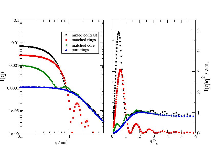
- jscatter.ff.flowerlikeMicelle(q, R, Nring, Nmonomer, monomerVolume, a, nu=0.5, ringSLD=6.4e-05, sphereSLD=0.0004186, solventSLD=0.0006335, d=1)[source]
Scattering of a sphere surrounded by gaussian rings as model for grafted ring polymers on sphere e.g. a micelle build of triblocks.
Compared to the
sphereGaussianCorona()here we use the polymer ring as a template for grafted chains.- Parameters:
- q: array of float
Wavevectors in unit 1/nm
- Rfloat
Sphere radius in unit nm
- dfloat, default 1
Ring centre located d*Rg away from the sphere surface. For ring Rg see
ringPolymer().- Nringfloat
Number of rings at the surface (aggregation number)
- Nmonomerint
Monomer number in single ring.
- afloat
Monomer segment length in units nm. See
ringPolymer()- monomerVolumefloat
Monomer volume in unit nm³.
- nufloat, default=0.5
ν is the excluded volume parameter (see ringPolymer), which is related to the Porod exponent d as ν = 1/d and [5/3 <= d <= 3].
fully swollen ring ν = 3/5 (good solvent)
for Gaussian ring ν = 1/2 (theta solvent)
collapsed ring ν = 1/3 (bad solvent)
- ringSLDfloat
Scattering length density of ring in bulk \(\rho_{ring}\). unit nm^-2. default hPEG = 0.64*1e-6 A^-2 = 0.64*1e-4 nm^-2
- sphereSLDfloat
Scattering length density of sphere.unit nm^-2. default SiO2 = 4.186*1e-6 A^-2 = 4.186*1e-4 nm^-2
- solventSLDfloat
Scattering length density of solvent. unit nm^-2. default D2O = 6.335*1e-6 A^-2 = 6.335*1e-4 nm^-2
- Returns:
- dataArray
- Columns [q,Iq,Iqring]
.ringRg
.sphereRadius
.Nring
.ringdistancefactor
.ringVolume
.ringSLD
.sphereSLD
.solventSLD
and … more
Notes
We calc in analogy to [1] but using ring formfactors
\[\begin{split}F(Q) &= F_{sphere}(Q,R) \\ &+ N_{ring} F_{ring}(Q, N,a,\nu) \\ &+ 2N_{ring} F_{a,sphere}(Q,R) F_{a,ring}(Q, N,a,\nu) sin(Q(R + d R_g))/(Q(R + d R_g)) \\ &+ N_{ring} * (N_{ring} - 1) F_{ring}(Q, N,a,\nu) (sin(Q(R + d R_g)) / (Q(R + d R_g)))^2\end{split}\]with formfactors \(F(Q,)=F^2_a(Q,)\) of a sphere \(F_{sphere}(Q,R)\) and the ring \(F_{ring}(Q, N,a,\nu)\)
The formfactor amplitudes
\[\begin{split}F_{a,sphere}(Q,R) &= \rho_{sphere} V_{sphere}\left[\frac{3(sin(qR) - qR cos(qR))}{(qR)^3}\right] \\ F_{a,ring}(Q, N,a,\nu) &= \rho_{ring} V_{ring} (F_{ring}(Q, N,a,\nu))^{0.5}\end{split}\]with the ring formfactor described in
ringPolymer().Explicitly we use the root of the ring formfactor for a ring formfactor amplitude similar to
sphereGaussianCorona(). The ring formfactor is always positive and does not cross zero.The defaults values result in a silica sphere with hPEG grafted rings at the surface in D2O.
References
[1]Form factors of block copolymer micelles with spherical, ellipsoidal and cylindrical cores Pedersen J. Journal of Applied Crystallography 2000 vol: 33 (3) pp: 637-640
Examples
import jscatter as js
q=js.loglist(0.1,5,100)
p=js.grace(1.4,1)
p.multi(1,2)
for rsld, ssld, le in [[1e-4,4e-4,'mixed contrast'],
                       [6e-4,4e-4,'matched rings'],
                       [1e-4,6e-4,'matched core']]:
   fq = js.ff.flowerlikeMicelle(q,R=4,Nring=10,Nmonomer=66,monomerVolume=0.1,a=0.5,
                       ringSLD=rsld,sphereSLD=ssld, solventSLD=6e-4)
   p[0].plot(fq, le=le)
   # Kratky plot
   p[1].plot(fq.X*fq.ringRg,fq.Y*fq.X**2 *1e4)
p[0].plot(fq.X,fq.Nring * fq._Iqring,le='pure rings')
p[1].plot(fq.X*fq.ringRg,fq.Nring * fq._Iqring*fq.X**2 *1e4)

p[0].yaxis(label='I(q)', charsize=1.5,scale='l',min=1e-6,max=0.1)
p[0].xaxis(label=r'q / nm\S-1',scale='l')
p[1].yaxis(label=[r'I(q)q\S2\N / a.u.',1.5,'opposite'],scale='n',min=0,max=5.5)
p[1].xaxis(label=r'q R\sg',scale='n')

p[0].legend(x=0.7,y=0.03)
#p.save(js.examples.imagepath+'/flowerlikeMicelle.jpg',size=[1.4,1],dpi=600)
In the Kratky plot we see the characteristic ring maximum around \(qR_{g,ring} \approx 2\).
This is visible for small rings, here Rg≈1.2 nm, and might interfere with the oscillations due to the core scattering for smaller cores. For \(\nu>0.5\) it becomes more difficult to see the maximum.
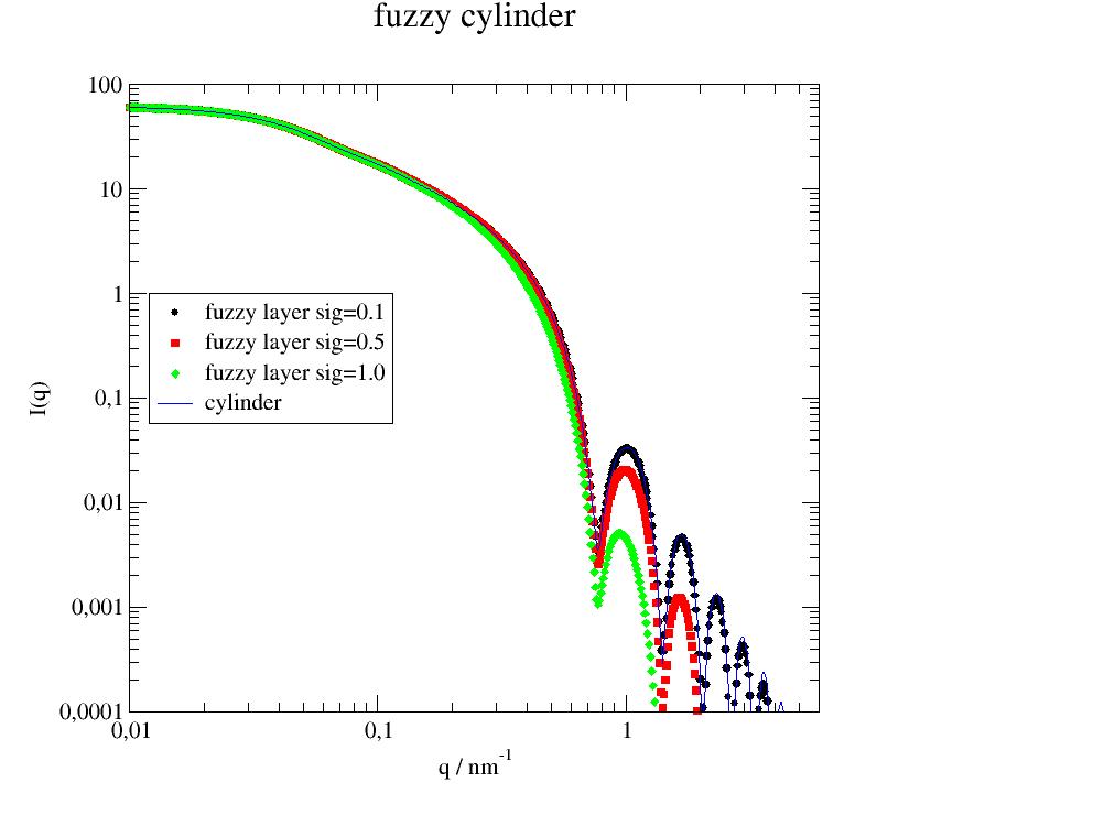
- jscatter.ff.fuzzyCylinder(q, L, radius, sigmasurf, SLD=0.001, solventSLD=0, alpha=None, nalpha=90)[source]
Cylinder with a fuzzy surface as in fuzzySphere averaged over axis orientations.
- Parameters:
- qarray
Wavevectors, units 1/nm
- Lfloat
Length of cylinder, units nm. L=0 infinite cylinder.
- radiusfloat
Radius of the cylinder in nm.
- sigmasurffloat
Sigmasurf is the width of the smeared particle surface in units nm.
- SLDfloat, default about SiO2 in H2O
Scattering length density of cylinder in nm^-2. SiO2 = 4.186*1e-6 A^-2 = 4.186*1e-4 nm^-2
- solventSLDfloat
Scattering length density of surrounding solvent in nm^-2. D2O = 6.335*1e-6 A^-2 = 6.335*1e-4 nm^-2
- alphafloat, [float,float], default [0,pi/2]
Orientation, angle between the cylinder axis and the scattering vector q in units rad. 0 means parallel, pi/2 is perpendicular If alpha =[start,end] is integrated between start,end start > 0, end < pi/2
- nalphaint, default 30
Number of points in Gauss integration along alpha.
- Returns:
- dataArray
- Columns [q ,Iq ]
.cylinderVolume
.radius
.cylinderLength
.alpha
.SLD
.solventSLD
.modelname
References
The models is derived from the
sphereFuzzySurface(). Similar is used in for the core in[1]Lund et al, Soft Matter, 2011, 7, 1491
Examples
import jscatter as js
import numpy as np
q=js.loglist(0.01,5,500)

p=js.grace()
for sig in [0.1,0.5,1]:
    fc=js.ff.fuzzyCylinder(q,L=100,radius=5,sigmasurf=sig)
    p[0].plot(fc,le='fuzzy layer sig={0:.1f}'.format(sig))
cc=js.ff.cylinder(q,L=100,radius=5)
p.plot(cc,li=[1,1,4],sy=0,le='cylinder')
p.yaxis(label='I(q)',scale='l',min=1e-4,max=1e2)
p.xaxis(label='q / nm\S-1',scale='l',min=0.01,max=6)
p.title('fuzzy cylinder')
p.legend(x=0.012,y=1)
#p.save(js.examples.imagepath+'/fuzzyCylinder.jpg')
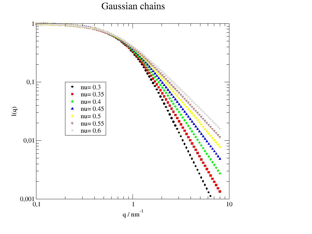
- jscatter.ff.gaussianChain(q, Rg, nu=0.5)[source]
General formfactor of a gaussian polymer chain with excluded volume parameter.
For nu=0.5 this is the Debye model for Gaussian chain in theta solvent. nu>0.5 for good solvents,nu<0.5 for bad solvents. For absolute scattering see introduction formfactor (ff).
- Parameters:
- qarray
Scattering vector, unit e.g. 1/A or 1/nm
- Rgfloat
Radius of gyration, units in 1/unit(q)
- nufloat, default=0.5
ν is the excluded volume parameter, which is related to the Porod exponent d as ν = 1/d and [5/3 <= d <= 3].
fully swollen chains ν = 3/5 (good solvent)
for Gaussian chains ν = 1/2 (theta solvent)
collapsed chains ν = 1/3 (bad solvent)
- Returns:
- dataArray
Columns [q,Fq]
.Rg
.nu excluded volume parameter
Notes
\(R_g^2=\frac{l^2 N^{2\nu}}{(2\nu+1)(2\nu+2)}\) with monomer length l and monomer number N.
With \(U=Q^2l^2N^{2\nu}/6 =Q^2R_g^2(2\nu+1)(2\nu+2)/6\) and \(\gamma_{inc}\) as lower incomplete gamma function
\[F(Q) = \frac{1}{\nu U^{\frac{1}{2\nu}}} \gamma_{inc}(\frac{1}{2\nu}, U) - \frac{1}{\nu U^{\frac{1}{\nu}}} \gamma_{inc}(\frac{1}{\nu}, U)\]For \(\nu=0.5\) this yields the Debye function
\[F(Q) = 2\frac{exp(-U)-1+U}{U^2}\]with \(U=(qR_g)^2\) .
The absolute scattering is proportional to \(b^2 N^2=b^2 (R_g/l)^{1/\nu}\) with monomer number \(N\) and monomer scattering length \(b\).
From [1]: “Note that this model describing polymer chains with excluded volume applies only in the mass fractal range ([5/3 <= d <= 3]) and does not apply to surface fractals ([3 < d < 4]). It does not reproduce the rigid-rod limit (d = 1) because it assumes chain flexibility from the outset, nor does it describe semi-flexible chains ([1 < d < 5/3]). “
This model should be favoured compared to the Beaucage model as it is not an artificial connection between two regimes.
References
[1]Analysis of the Beaucage model Boualem Hammouda J. Appl. Cryst. (2010). 43, 1474–1478 http://dx.doi.org/10.1107/S0021889810033856
[2]SANS from homogeneous polymer mixtures: A unified overview. Hammouda, B. in Polymer Characteristics 87–133 (Springer-Verlag, 1993). doi:10.1007/BFb0025862
Examples
import jscatter as js
import numpy as np
q=js.loglist(0.1,8,100)
p=js.grace()
for nu in np.r_[0.3:0.61:0.05]:
   iq=js.ff.gaussianChain(q,2,nu)
   p.plot(iq,le='nu= $nu')
p.yaxis(label='I(q)',scale='l',min=1e-3,max=1)
p.xaxis(label='q / nm\S-1',scale='l')
p.legend(x=0.2,y=0.1)
p.title('Gaussian chains')
#p.save(js.examples.imagepath+'/gaussianChain.jpg')
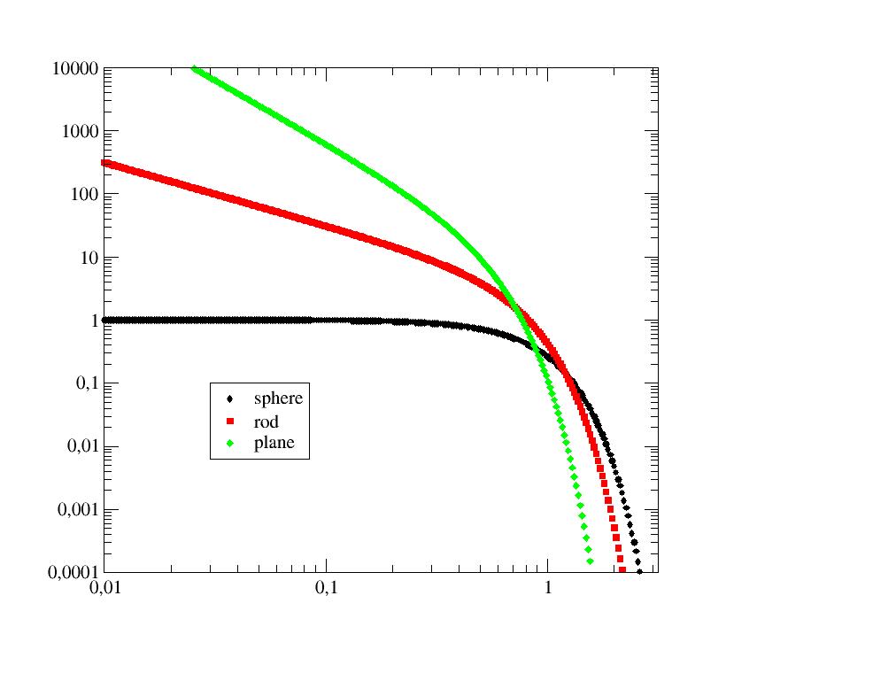
- jscatter.ff.genGuinier(q, Rg=1, A=1, alpha=0)[source]
Generalized Guinier approximation for low wavevector q scattering q*Rg< 1-1.3
For absolute scattering see introduction formfactor (ff).
- Parameters:
- qarray of float
Wavevector
- Rgfloat
Radius of gyration in units=1/q
- alphafloat
Shape [α = 0] spheroid, [α = 1] rod-like [α = 2] plane
- Afloat
Amplitudes
- Returns:
- dataArray
Columns [q,Fq]
Notes
- Quantitative analysis of particle size and shape starts with the Guinier approximations.
For three-dimensional objects the Guinier approximation is given by \(I(q) = A e^{-Rg^2q^2/3}\)
This approximation can be extended also to rod-like and plane objects by \(I(q) =(\alpha \pi q^{-\alpha}) A e^{-Rg^2q^2/(3-\alpha) }\)
If the particle has one dimension of length L that is much larger than the others (i.e., elongated, rod-like, or worm-like), then there is a q range such that qR_c < 1 << qL, where α = 1.
References
[1]Form and structure of self-assembling particles in monoolein-bile salt mixtures Rex P. Hjelm, Claudio Schteingart, Alan F. Hofmann, and Devinderjit S. Sivia J. Phys. Chem., 99:16395–16406, 1995
Examples
import jscatter as js
import numpy as np
q=js.loglist(0.01,5,300)
spheroid=js.ff.genGuinier(q, Rg=2, A=1, alpha=0)
rod=js.ff.genGuinier(q, Rg=2, A=1, alpha=1)
plane=js.ff.genGuinier(q, Rg=2, A=1, alpha=2)
p=js.grace()
p.plot(spheroid,le='sphere')
p.plot(rod,le='rod')
p.plot(plane,le='plane')
p.yaxis(scale='l',min=1e-4,max=1e4)
p.xaxis(scale='l')
p.legend(x=0.03,y=0.1)
#p.save(js.examples.imagepath+'/genGuinier.jpg')
- jscatter.ff.guinier(q, Rg=1, A=1)[source]
Classical Guinier
\(I(q) = A e^{-Rg^2q^2/3}\) see genGuinier with alpha=0
- Parameters:
- q :array
- Afloat
- Rgfloat
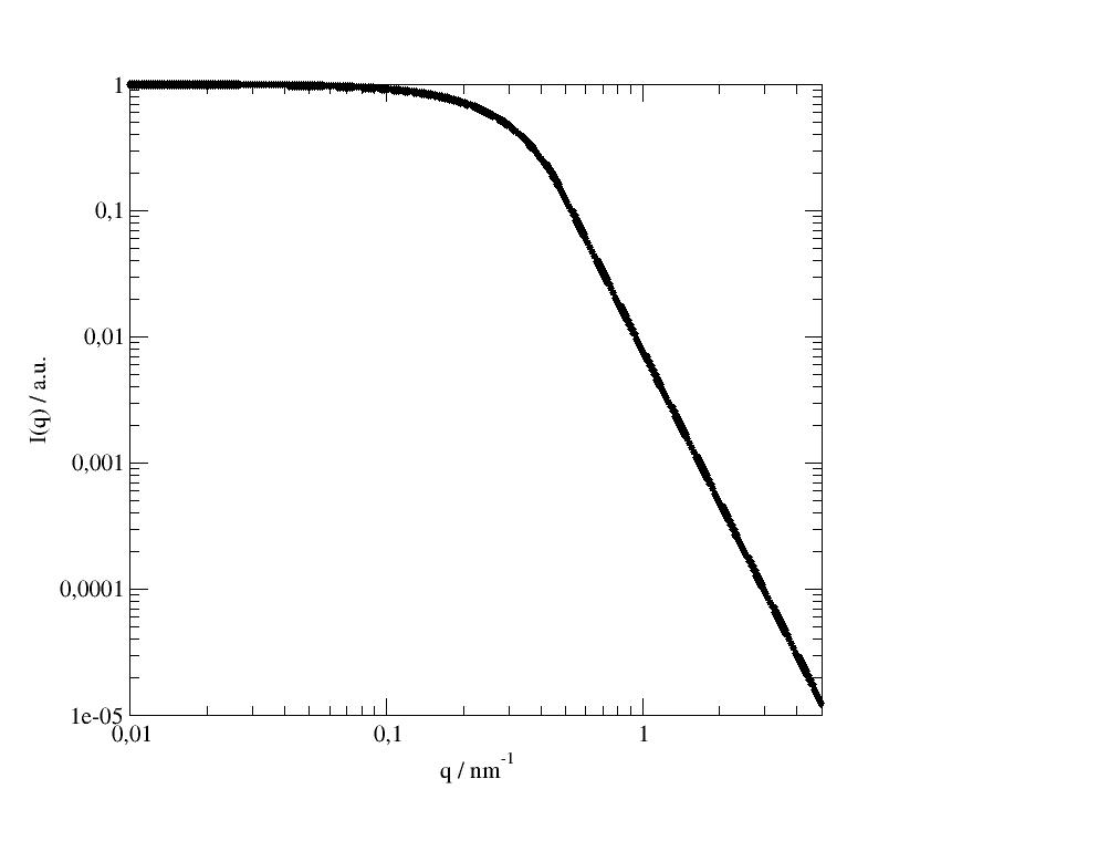
- jscatter.ff.guinierPorod(q, Rg, s, I0, d)[source]
Generalized Guinier-Porod Model with high Q power law.
An empirical model connecting the Guinier model with a transition to Porod scattering at high Q.
- Parameters:
- qfloat
Wavevector in units of 1/nm
- Rgfloat
Radii of gyration in units nm.
- sfloat
- Dimensionality parameter describing the low Q region.
0 spheres globular
1 rods, linear
2 lamella planar
- dfloat
Porod exponent describing the high Q slope.
- I0float
Intensity, named G in [1].
- Returns:
- dataArray
Columns [q, Iq] Iq scattering intensity
Notes
Equ. 3 in [1] as:
\[ \begin{align}\begin{aligned}I(Q) &= \frac{G}{Q^s}exp\big(\frac{-Q^2R_g^2}{3-s}\big) \; for Q \leq Q_1\\I(Q) &= \frac{D}{Q^d} \; for Q \geq Q_1\end{aligned}\end{align} \]with equ 4
\[ \begin{align}\begin{aligned}Q_1 &= \frac{1}{R_g} \big( \frac{(d-s)(3-s)}{2} \big)^{1/2}\\D &= G exp(\frac{-Q_1^2R_g^2}{3-s})Q_1^{d-s}\end{aligned}\end{align} \]References
Author M. Kruteva JCNS 2019
Examples
import jscatter as js
q=js.loglist(0.01,5,300)
I=js.ff.guinierPorod(q,s=0,Rg=5,I0=1,d=4)
p=js.grace()
p.plot(I)
p.xaxis(scale='l',label='q / nm\S-1')
p.yaxis(scale='l',label='I(q) / a.u.')
#p.save(js.examples.imagepath+'/guinierPorod.jpg')
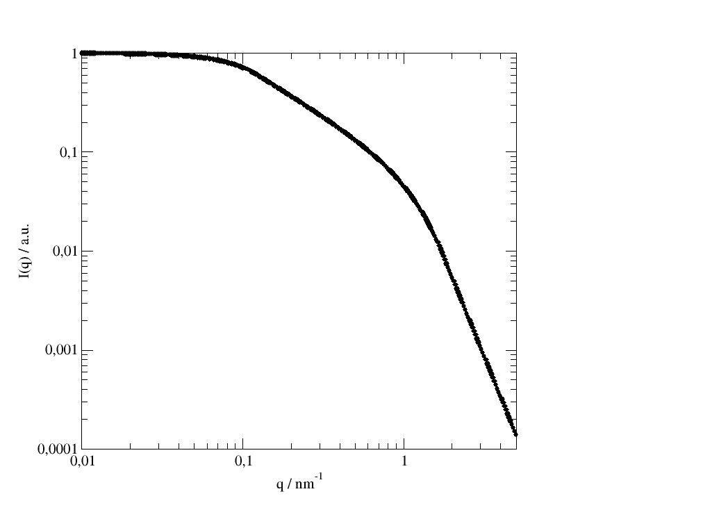
- jscatter.ff.guinierPorod3d(q, Rg1, s1, Rg2, s2, G2, dd)[source]
Generalized Guinier-Porod Model with high Q power law with 3 length scales.
An empirical model connecting the Guinier model with a transition to Porod scattering at high Q. The model represents the most general case containing three Guinier regions [1].
- Parameters:
- qfloat
Wavevector in units of 1/nm
- Rg1float
Radii of gyration for the short size of scattering object in units nm.
- Rg2float
Radii of gyration for the overall size of scattering object in units nm.
- s1float
Dimensionality parameter for the short size of scattering object (s1=1 for a cylinder)
- s2float
Dimensionality parameter for the overall size of scattering object (s2=0 for a cylinder)
- G2float
Intensity for q=0.
- dfloat
Porod exponent
- Returns:
- dataArray
- Columns [q,Iq]
Iq scattering intensity
Notes
Equ. 5 in [1] as:
\[ \begin{align}\begin{aligned}I(Q) &= \frac{G_2}{Q^{s_2}} exp\big(\frac{-Q^2R_{g2}^2}{3-s_2}\big) \; for Q \leq Q_2\\I(Q) &= \frac{G_1}{Q^{s_1}} exp\big(\frac{-Q^2R_{g1}^2}{3-s_1}\big) \; for Q_2 \leq Q \leq Q_1\\I(Q) &= \frac{D}{Q^d} \; for Q \geq Q_1\end{aligned}\end{align} \]with equ 4
\[ \begin{align}\begin{aligned}Q_1 &= \frac{1}{R_{g1}} \big( \frac{(d-s_1)(3-s_1)}{2} \big)^{1/2}\\D &= G_1 exp(\frac{-Q_1^2R_{g1}^2}{3-s_1})Q_1^{d-s_1}\\Q_2 &= \big[frac{s_1-s_2}{\frac{2}{3-s_2}R_{g2}^2 - \frac{2}{3-s_1}R_{g1}^2 } \big]^{1/2}\\G_2 &= G_1 exp\big[ -Q_2^2 \big(\frac{R_{g1}^2}{3-s_1} - \frac{R_{g2}^2}{3-s_2} \big) \big] Q_2^{s_2-s_1}\end{aligned}\end{align} \]For fitting limit parameters to \(3>s_1>s_2\) and \(R_{g2} >R_{g1}\). For more details see [1]
For a cylinder with length L and radius R (see [1]) \(R_{g2} = (L^2/12+R^2/2)^{\frac{1}{2}}\) and \(R_{g1}=R/\sqrt{2}\)
References
Author M. Kruteva JCNS 2019
Examples
import jscatter as js
q=js.loglist(0.01,5,300)
I=js.ff.guinierPorod3d(q,Rg1=1,s1=1,Rg2=10,s2=0,G2=1,dd=4)
p=js.grace()
p.plot(I)
p.xaxis(scale='l',label='q / nm\S-1')
p.yaxis(scale='l',label='I(q) / a.u.')
#p.save(js.examples.imagepath+'/guinierPorod3d.jpg')
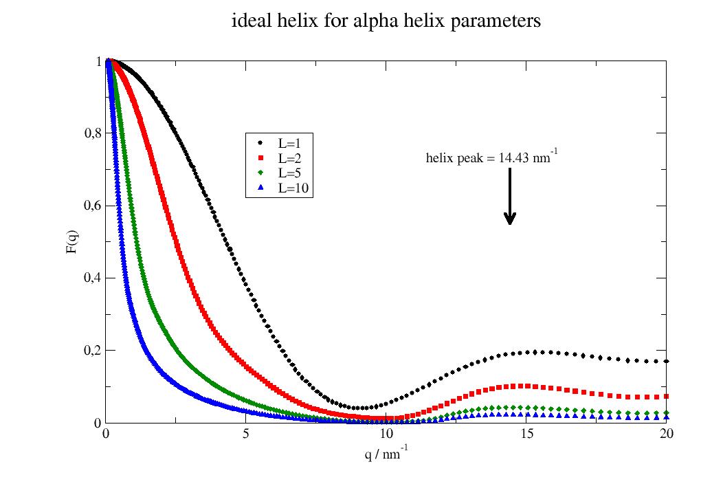
- jscatter.ff.idealHelix(q, L=3, R=0.3, P=0.54, n=10.8, Rot=None)[source]
Ideal helix like the protein α-helix.
- Parameters:
- qarray, 1xN or 3xN
Scattering vector in units 1/nm. If 1 dim array the spherical average is returned. For 3xN array as xyz coordinates no average is performed (for 2D images).
- Lfloat
Total helix length in nm. \(L = N P/n_p\)
with Number of amino acids N, pitch P and atomsper pitch \(n_p\)
- Rfloat
Radius of the helix in nm.
- Pfloat
Pitch as repeating distance along helix.
- nfloat
Number of atoms per pitch
- Rotarray 3x3 or [float,float]
- Rotation matrix describing the orientation of the helix axis. None=[0,0] means axis along Z=axis.
As rotation matrix it describes the rotation of a helix oriented along the Z-axis.
As 2 floats it describes the helix axis rotation (parallel Z-Axis) first around the Y-axis, second around the Z-axis in units degree.
See second example.
- Returns:
- dataArray dim 2xN or 4xN dependent on q dimension.
References
[1]Conformation of Peptides in Lipid Membranes Studied by X-Ray Grazing Incidence Scattering A. Spaar, C. Münster, and T. Salditt Biophysical Journal 87, 396–407 (2004) doi: 10.1529/biophysj.104.040667
[2]Atomic Coordinates and Structure Factors for Two Helical Configurations of Polypeptide Chains L. Pauling, R.B. Corey Proc. Natl. Acad. Sci. USA. 37, 235–240 (1951). doi: 10.1073/pnas.37.5.235
Examples
Isotropic scattering of an ideal helix with random orientation. The helix peak is located at [1]
\[q_z = \frac{2\pi}{P} \; q_{||}=\frac{5\pi}{8R}\]with \(q_z\) along the helix axis and \(q_{||}\) perpendicular assuming average around the axis. The pattern is characteristic for helices and used by Pauling and Corey (1951) to identify the α-helix [2]
import jscatter as js
q = js.loglist(0.1,20,300)
p = js.grace()
for L in [1, 2, 5,10]:
    fq = js.ff.idealHelix(q,L=L, R=0.23, P=0.54, n=3.6)
    p.plot(fq,le=f'L={L}')
p.yaxis(label='F(q)')
p.xaxis(label='q / nm\S-1')
p.title('ideal helix for alpha helix parameters')
p.legend(x=5,y=0.8)
qh = fq.helixpeak_radial
p[0].line(qh,0.7,qh,0.55,4,arrow=2,arrowlength=2)
p[0].text(f'helix peak = {qh:.2f} nm\S-1',x=qh-3,y=0.72 )
# p.save(js.examples.imagepath+'/idealhelix0.jpg')
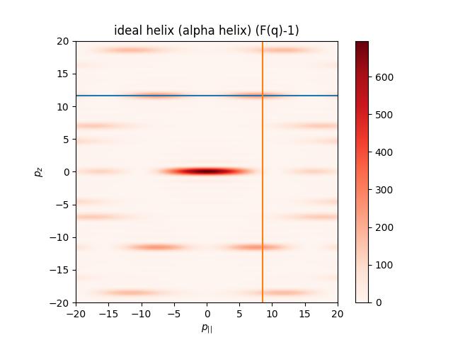
import jscatter as js
from scipy.spatial.transform import Rotation

# helix axis rotation
R=Rotation.from_euler('YZ',[90,0],degrees=True).as_matrix()
# generate 3dim q like Ewald sphere with ki=[0,0,1].
qe = js.formel.qEwaldSphere(q=[20],N=200,typ='cart', wavelength=0.15)

fq = js.ff.idealHelix(qe, L=6, R=0.23, P=0.54, n=3.6, Rot=R)  # same as Rot=[90,0]
fig=js.mpl.contourImage(fq, scale='lin', invert_yaxis=1, colorMap= 'Reds')
fig.axes[0].plot([-20,20], [fq.helixpeak_z]*2)
fig.axes[0].plot( [fq.helixpeak_p]*2,[-20,20])
fig.axes[0].set_title('ideal helix (alpha helix) (F(q)-1)')
fig.axes[0].set_xlabel(r'$p_{||}$')
fig.axes[0].set_ylabel(r'$p_z$')
# fig.savefig(js.examples.imagepath+'/idealhelix.jpg')
The larger q range shows the typical helical X structure. To see this in SAXS/WAXS the helix needs to be large.
import jscatter as js
from scipy.spatial.transform import Rotation

# helix axis rotation
R=Rotation.from_euler('YZ',[90,0],degrees=True).as_matrix()
# generate 3dim q like Ewald sphere with ki=[0,0,1].
qe = js.formel.qEwaldSphere(q=[60],N=200,typ='cart', wavelength=0.015)

fq = js.ff.idealHelix(qe, L=6, R=0.23, P=0.54, n=3.6, Rot=R)  # same as Rot=[90,0]
fig=js.mpl.contourImage(fq, invert_yaxis=1, colorMap= 'Reds')
fig.axes[0].plot([-20,20], [fq.helixpeak_z]*2)
fig.axes[0].plot( [fq.helixpeak_p]*2,[-20,20])
fig.axes[0].set_title('ideal helix (alpha helix) (F(q)-1)')
fig.axes[0].set_xlabel(r'$p_{||}$')
fig.axes[0].set_ylabel(r'$p_z$')
# fig.savefig(js.examples.imagepath+'/idealhelix1.jpg')

- jscatter.ff.inhomogeneousCylinder(q, Rcore, L, Rdrop, Ddrops, coreSLD, dropSLD=None, solventSLD=0, rms=0, typ='drop', distribution='quasirandom', h=0, nconf=34, show=False, **kwargs)[source]
Scattering of a caped cylinder filled with droplets.
The model described caped cylinder particle filled with drops. Drops are added only in the core volume (drop center < Rcore) extending outside if radius is large enough.
The model uses cloudscattering and the source can be used as a template for more specific models.
- Parameters:
- qarray
Wavevectors in units 1/nm.
- Rcorefloat
Core radius in nm.
- Lfloat
Cylinder length in units nm.
- Rdropfloat
Radius of small drops in units nm.
- Ddropsint
Average distance between drops in nm.
- hfloat, default=None
Geometry of the caps with cap radii \(R_i=(r_i^2+h^2)^{0.5}\). See multiShellCylinder. h is distance of cap center with radius R from the flat cylinder cap and r as radii of the cylinder shells.
None: No caps, flat ends as default.
0: cap radii equal cylinder radii (same shellthickness as cylinder shells)
>0: cap radius larger cylinder radii as barbell
<0: cap radius smaller cylinder radii as lens caps
- shellthicknessfloat
Optional a shellthickness (units nm) to add an outer shell around the core with scattering length shellSLD.
- coreSLD,dropSLD,shellSLD: float
Scattering length of core and drops (optional shell) in unit 1/nm².
- solventSLDfloat
Solvent scattering length density in unit 1/nm².
- typ‘gauss’, ‘coil’, default=’drop’
- Type of the drops
‘drop’ sphere with dropSLD. Drop scattering length is dropSLD*4/3pi Rdrop**3 .
‘coil’ polymer coils. Coil scattering length is dropSLD*4/3pi Rdrop**3 .
- ‘gauss’ Gaussian function \(b_i(q)=b V exp(-\pi V^{2/3}q^2)\) with \(V = 4\pi/3 R_{drop}^3\) .
According to [1] the atomic scattering amplitude can be represented by gaussians with the volume representing the displaced volume (e.g using the Van der Waals radius)
- distribution‘random’,’fcc’, default=’quasirandom’
- Distribution of drops as :
‘random’ random points. difficult for fitting as the configuration changes for each call.
- ‘quasirandom’ quasirandom distribution of drops in sphere.
The distribution is always the same if repeated several times. quasirandom is a bit more homogeneous than random with less overlap of drops.
‘fcc’ a fcc lattice.
- rmsfloat, default=0
Root mean square displacement :math:`langleu^2rangle^{0.5} of the positions in cloud as random (Gaussian) displacements in nm. Displacement u is random for each orientation in sphere scattering.
- nconfint, default=34
Determines how many configurations are averaged. For ‘fcc’ it determines the number of angular orientations, a lower number is already sufficient. For others it is the number of independent configurations, each averaged over 5 angular orientations.
- showbool
Show a 3D image of a configuration using matplotlib. This returns a figure handle.
- Returns:
- dataArray
- Columns [q; fq; fq_cyl; fq_drops’]
attributes from call
.Ndrop number of drops in caped cylinder
.dropVolumeFraction \(=N_{drop}V_{drop}/V_{caped cylinder}\)
Notes
The scattering amplitude \(F_{a,cyl}(q,\alpha)\) of a caped cylinder is calculated (see multiShellCylinder for a reference).
At the positions of drops inside of the caped cylinder core additional drops are positioned with respective scattering amplitudes \(F_{a,drop}(q)\) according to typ.
Positions are distributed as ‘fcc’, ‘random’ or ‘quasirandom’.
The combined scattering amplitude is \(F_a(q,\alpha) = F_{a,cyl}(q,\alpha) + \sum_i e^{iqr_i}F_{a,drop}\) and \(F(q) = \int F_a(q,\alpha)F^*_a(q,\alpha) d\alpha\)
If drops overlap the overlap volume is counted double assuming an area of higher density. Drop volume can extend to the outside of the large sphere. Rdrop is explicitly not limited to allow this.
References
[1]An improved method for calculating the contribution of solvent to the X-ray diffraction pattern of biological molecules Fraser R MacRae T Suzuki E IUCr Journal of Applied Crystallography 1978 vol: 11 (6) pp: 693-694
Examples
Comparing sphere and filled sphere. The inhomogeneous filling filled up the characteristic sphere minima. Gaussian coil filling also removes the high q minima from small filling spheres.
import jscatter as js
q=js.loglist(0.01,5,300)
drop=-1
fig = js.ff.inhomogeneousCylinder(q=q,Rcore=10,L=50, Rdrop=2.4,h=0, Ddrops=6,coreSLD=1,dropSLD=drop,show=1,typ='coil',distribution='fcc')
bb=fig.axes[0].get_position()
fig.axes[0].set_title('inhomogeneous filled cylinder \nwith volume fraction 0.53')
fig.axes[0].set_position(bb.shrunk(0.5,0.9))
ax1=fig.add_axes([0.58,0.1,0.4,0.85])
ihC= js.ff.inhomogeneousCylinder(q=q,Rcore=10,L=50, Rdrop=2.4,h=0, Ddrops=6,coreSLD=1,dropSLD=drop,show=0,typ='coil',distribution='fcc')
ax1.plot(ihC.X,ihC.Y,label='doped cylinder')
ax1.plot(ihC.X,ihC._fq_cyl,label='homogeneous cylinder')
ax1.plot(ihC.X,ihC._fq_drops,label='only drops')
ax1.set_yscale('log')
ax1.set_xscale('log')
ax1.legend()
fig.set_size_inches(8,4)
#fig.savefig(js.examples.imagepath+'/filledCylinder.jpg')
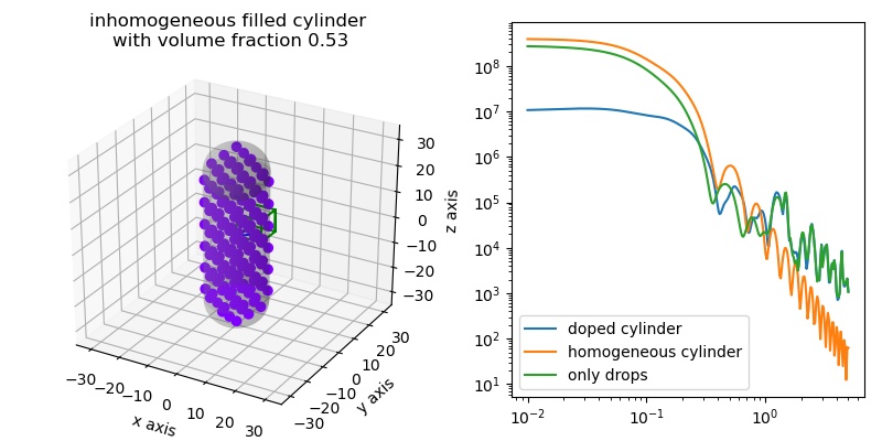
- jscatter.ff.inhomogeneousSphere(q, Rcore, Rdrop, Ddrops, coreSLD, dropSLD=None, solventSLD=0, rms=0, typ='drop', distribution='quasirandom', relError=100, show=False, **kwargs)[source]
Scattering of a core shell sphere filled with droplets of different types.
The model described spherical particle filled with particles as drops or coils as described in [1]. Drops are added in the internal volume extending outside if radius is large enough.
The model uses cloudscattering and the source can be used as a template for more specific models.
- Parameters:
- qarray
Wavevectors in units 1/nm.
- Rcorefloat
Core radius in nm.
- Rdropfloat
Radius of small drops in units nm.
- Ddropsint
Average distance between drops in nm.
- shellthicknessfloat
Optional a shellthickness (units nm) to add an outer shell around the core with scattering length shellSLD.
- coreSLD,dropSLD,shellSLD: float
Scattering length of core and drops (optional shell) in unit nm^-2.
- solventSLDfloat
Solvent scattering length density in unit nm^-2.
- typstring = (‘drop’, ‘coil’, ‘gauss’) + ‘core’ or/and ‘shell’, default ‘core’
Type of the drops and were to place them. See cloudscattering for types. If the string contains ‘core’, ‘shell’ the drops are placed in one or both of core and shell.
‘drop’ sphere with dropSLD
- ‘coil’ gaussian coils. Coil scattering length is \(F_a(q=0) = dropSLD*4/3pi Rdrop**3\)
with formfactor amplitude of Gaussian chain.
- ‘gauss’ Gaussian function \(b_i(q)=b V exp(-\pi V^{2/3}q^2)\) with \(V = 4\pi/3 R_{drop}^3\) .
According to [2] the atomic scattering amplitude can be represented by gaussians with the volume representing the displaced volume (e.g using the Van der Waals radius)
- distribution‘random’,’quasirandom’,’fcc’, default=’quasirandom’
- Distribution of drops as :
‘random’ random points. Difficult for fits as the configuration changes with each call.
- ‘quasirandom’ quasirandom distribution of drops in sphere.
The distribution is always the same if repeated several times. quasirandom is a bit more homogeneous than random with less overlap of drops.
‘fcc’ a fcc lattice
- rmsfloat, default=0
Root mean square displacement \(\langle u^2\rangle ^{0.5}\) of the positions in cloud as random (Gaussian) displacements in nm. Displacement u is random for each orientation in sphere scattering.
- relErrorfloat
Determines calculation method. See
cloudScattering()- showbool
Show a 3D image using matplotlib.
- Returns:
- dataArray
- Columns [q, Fq, Fq coreshell]
attributes from call
.Ndrop number of drops in sphere
.dropVolumeFraction \(=N_{drop}R_{drop}^3/R_{core}^3\)
Notes
- The models uses cloudscattering with multi component particle distribution.
At the center is a large sphere located.
At the positions of droplets inside of the large sphere additional small spheres or gaussian coils are positioned.
cloudscattering is used to calculate the respective scattering including all cross terms.
If drops overlap the overlap volume is counted double assuming an area of higher density. Drop volume can extend to the outside of the large sphere. The Rdrop is explicitly not limited to allow this.
References
[1]Controlled LCST Behavior and Structure Formation of Alternating Amphiphilic Copolymers in Water. Kostyurina, E. et al Macromolecules, 55(5), 1552–1565 (2022). https://doi.org/10.1021/acs.macromol.1c02324
[2]An improved method for calculating the contribution of solvent to the X-ray diffraction pattern of biological molecules Fraser R MacRae T Suzuki E IUCr Journal of Applied Crystallography 1978 vol: 11 (6) pp: 693-694
Examples
Comparing sphere and filled sphere. The inhomogeneous filling filled up the characteristic sphere minima. Gaussian coil filling also removes the high q minima from small filling spheres.
import jscatter as js
q=js.loglist(0.03,5,300)
fig = js.ff.inhomogeneousSphere(q=q,Rcore=20, Rdrop=5, Ddrops=11, coreSLD=0.001, dropSLD=2.5,show=1)
bb=fig.axes[0].get_position()
fig.axes[0].set_title('inhomogeneous filled sphere \nwith volume fraction 0.4')
fig.axes[0].set_position(bb.shrunk(0.5,0.9))
ax1=fig.add_axes([0.58,0.1,0.4,0.85])
R=2;D=2*R*1.1
drop = js.ff.inhomogeneousSphere(q=q,Rcore=20, Rdrop=R, Ddrops=D, coreSLD=0.1, dropSLD=1.5)
ax1.plot(drop.X,drop.Y, label='sphere with drops')
ax1.plot(drop.X,drop._sphere_fq,'--', label='sphere homogeneous')
drop1 = js.ff.inhomogeneousSphere(q=q,Rcore=20, Rdrop=R, Ddrops=D, rms=0.6, coreSLD=0.1, dropSLD=1.5)
ax1.plot(drop1.X,drop1.Y, label='sphere with drops rms=0.6')
drop2 = js.ff.inhomogeneousSphere(q=q,Rcore=20, Rdrop=R, Ddrops=D, rms=4, coreSLD=0.1, dropSLD=1.5)
ax1.plot(drop2.X,drop2.Y, label='sphere with drops rms=4')
drop3 = js.ff.inhomogeneousSphere(q=q,Rcore=20, Rdrop=R, Ddrops=D, rms=4, coreSLD=0.1, dropSLD=1.5, typ='coil')
ax1.plot(drop3.X,drop3.Y, label='sphere with polymer coil drops rms=4')
ax1.set_yscale('log')
ax1.set_xscale('log')
ax1.legend()
fig.set_size_inches(8,4)
#fig.savefig(js.examples.imagepath+'/filledSphere.jpg')
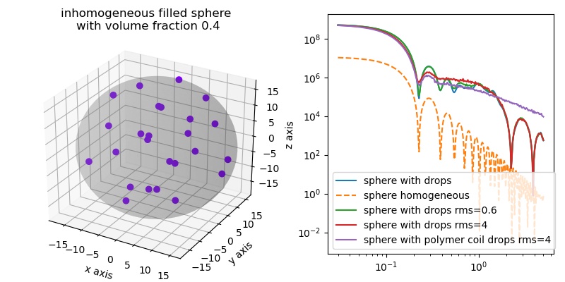
- jscatter.ff.linearChainORZ(q, N=100, l=1, fa=None, costheta=0.0)[source]
Formfactor of a linear polymer chain using optimized Rouse-Zimm approximation (ORZ).
The linear chain is decribed within the more general optimized Rouse-Zimm (ORZ) approximation introduced by Bixon and Zwanzig [3] [4] . See
solveOptimizedRouseZimm().We extend this here using bead scattering lengths for partial matching and allow individual bond correlations.
- Parameters:
- qarray
Scattering vectors in units 1/nm.
- Nint
Number of beads .
- lfloat, default = 0.38 nm (amino acid)
Bond length or Kuhn length in units nm.
- faNone, list of float
Scattering length of bead/monomer \(fa_i\). Can be used to match parts of the star to the solvent.
None : Equal 1 for all beads.
list: length N as scattering length of beads in sequence
- costhetafloat, list of float, 0 <= costheta < 1
Cos of bond correlation angle \(\langle \vec{l_i} \cdot \vec{l_j} \rangle /l^2 = cos(theta)\) between bonds \(l_i\) with \(0 \le cos(\theta) \le 1\).
costheta = 0 : FJC (freely jointed chain) model, no bond correlation, Rouse dynamics, No HI .
float \(0 < cos(\theta) \le 1\) : FRC (free rotating chain). With \(R_{ee} = Nl^2C_{\infty}=Nl^2 \frac{1+cos(\theta)}{1-cos(\theta)}\) .
list of float length N-2 : FRC with individual \(cos(\theta_i)\) for each pair of N-2 bonds.
costheta=([0.1]*24+[0.7]*24)for stretched beginning and flexible end of 50 beads.costheta=0.8 * np.cos(np.pi*np.r_[:1:(N-2)*1j])**2 + 0.1for flexible center and stretched ends.
For fitting encapsulate the model in a function where you parametrize your model for costheta.
- e.g. (from [5]_ p. 53) \(C_{\infty} | Kuhn length [A] | cos(theta)\)
polyisoprene 4.6 | 8.2 | 0.783
polyethylene oxide 6.7 | 11 | 0.85
polyethylene 7.4 | 14 | 0.865
atactic polystyrene 9.5 | 18 | 0.895
During fits use
limits(costheta=[None,None,0.001,0.999])to avoid singular matrices.
- Returns:
- fqdataArray
Formfactor a linear chain.
[q; fq]
columnname = ‘q;fq’
.costheta : costheta
.l : bondlength l
.N : Number of beads
.Rg : radius of gyration in nm
.Rg_red : reduced radius of gyration
Notes
See
solveOptimizedRouseZimm()for a description of the ORZ model with respective parameters.Here we use a linear chain with N beads and set elements \(U^{-1}_{ij} <0.001 \rightarrow 0\).
The inverse of the static bond correlation matrix \(U_{ij}^{-1} = \langle l_i\cdot l_j\rangle /l^2\) in dimesionless form is
\[\begin{split}U_{ij}^{-1} &= \delta_{i,j} &\text{ for uncorrelated bonds } \\ &= \prod_{n=i}^{j} g_n \; &\text{ for individual } g_i \text{ including constant g}\end{split}\]The transfer matrix M is
\[M = \delta_{i,j} - \delta_{i+1,j}\]References
[1]Static and Dynamic Structure Factors for Star Polymers in θ Conditions. Guenza, M. & Perico, A. Macromolecules 26, 4196–4202 (1993). https://doi.org/10.1021/ma00068a020
[2]A Local Approach to the Dynamics of Star Polymers. Guenza, M., Mormino, M. & Perico, A. Macromolecules 24, 6168–6174 (1991). https://doi.org/10.1021/ma00023a018
[3]Theoretical basis for the Rouse‐Zimm model in polymer solution dynamics. Zwanzig, R. The Journal of Chemical Physics 60, 2717–2720 (1974) https://doi.org/10.1063/1.1681433
[4]A hierarchy of models for the dynamics of polymer chains in dilute solution. Perico, A., Ganazzoli, F. & Allegra, G. The Journal of Chemical Physics 87, 3677–3686 (1987). https://doi.org/10.1063/1.452966
Examples
Here we examine how changig stiffness influences the form factor.
import jscatter as js
import numpy as np

q= js.loglist(0.02,5,100)

def stiffendschain(q, N, l=0.5, cosmin =0.05,cosmax=0.8):
   costheta = (cosmax-cosmin) * np.cos(np.pi*np.r_[:1:(N-2)*1j])**2 + cosmin
   fq = js.ff.linearChainORZ(q, N, l=0.5, costheta = costheta)
   return fq

p = js.grace()
p.multi(2,1)

for c,cs in enumerate(np.r_[0.:0.95:7j],1):
    fq = stiffendschain(q, 100, l=1, cosmin =0.1, cosmax=cs)
    p[0].plot(fq,li=[1,1,c],sy=0,le=f'Rg={fq.Rg:.2f} nm\\S-1')
    p[1].plot(fq.X,fq.Y*fq.X**2,li=[1,1,c],sy=0,le=f'Rg={fq.Rg:.2f} nm\\S-1')

p[0].xaxis(label='q / nm\S-1',scale='log')
p[1].xaxis(label='q / nm\S-1')
p[0].yaxis(label='I(Q)',scale='log',min=100,max=20000)
p[1].yaxis(label='I(Q)',scale='norm',min=0.01,max=2000)
p.title('chain with stiff ends ')
p[0].legend(x=0.02,y=6000,charsize=0.6)
# p.save(js.examples.imagepath+'/ORZ_linearstiffends_ff.png',size=(1.5,1.5),dpi=300)
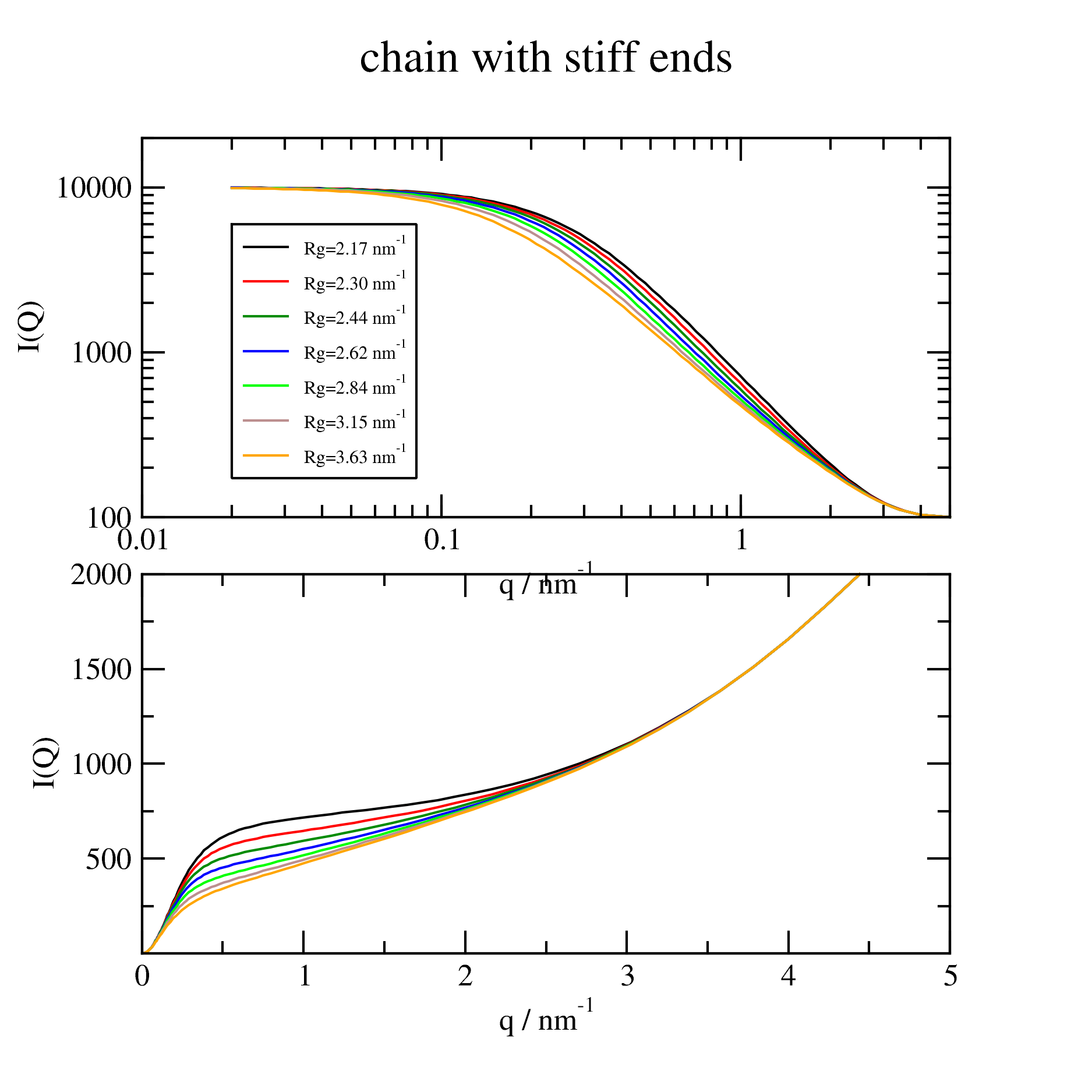
- jscatter.ff.linearPearls(q, N, R, l, pearlSLD, cr, n=1, relError=0, rms=0, ffpolydispersity=0, ncpu=0, smooth=7, shellthickness=0, shellSLD=0, solventSLD=0)[source]
Linear arranged pearls connected by gaussian chains in between them.
Large pearls are aligned in a line and connected by a polymer chain approximated as Gaussian coils. Increasing the number of connecting coils (reducing individual mass) result in an approximated linear connector. The model uses cloudscattering. The formfactor is normalized to 1. For absolute scattering see introduction formfactor (ff).
This model might be used as template to make models with with inhomogeneous pearls like hollow spheres or Gaussian coils as pearls just by changing the sphere formfactor and adjusting the geometry.
- Parameters:
- qarray, ndim= Nx1
Radial wavevectors in 1/nm
- Nint
Number of pearls
- Rfloat
Radius of uniform pearls in units nm.
- lfloat
Length of connectors in units nm. The distance between pearls center of mass is 2(R+shellD)+l
- pearlSLDfloat
Scattering length density in each pearl in units nm^-2. The pearl scattering length is volume*SLD (respectively the corresponding value for coreShell pearls)
- crfloat>=0
Virtual connector radius in units nm determining the connector scattering length. Describing the connector volume as a cylinder with scattering length density of the core the volume is \(V_c = \pi r_{cr}^2l\) and the scattering length is F_a(q=0)=V*pearlsSLD. The scattering length is distributed to n Gaussian coils. cr=0 means no connector.
- nint
Number of Gaussians coils in connector. The coils are equal distributed on pearl connecting lines with Rg=l/2/n that coils touch with a distance 2Rg and touch the radius of the pearls. Zero means no connector but pearls separated by l.
- shellthicknessfloat>=0
Optional a shellthickness \(d_{shell}\) (units nm) to add an outer shell around the pearl. The shellthickness is added to the distance between pearls.
- shellSLDfloat
Optional, scattering length density in each pearl shell in units nm^-2.
- solventSLDfloat
Solvent scattering length density in units nm^-2.
- relErrorfloat
- Determines calculation method.
- relError>1 Explicit calculation of spherical average with Fibonacci lattice on sphere
of 2*relError+1 points. Already 150 gives good results, more is better (see Examples)
- 0<relError<1 Monte Carlo integration on sphere until changes in successive iterations
become smaller than relError. (Monte carlo integration with pseudo random numbers, see sphereAverage). This might take long for too small error.
- relError=0 The Debye equation is used (no asymmetry factor beta, no rms, no ffpolydispersity).
Computation is of order \(N^2\) opposite to above which is order \(N\). For about 1000 particles same computing time,for 500 Debye is 4 times faster than above. If beta, rms or polydispersity is needed use above.
- rmsfloat, default=0
Root mean square displacement \(\langle u^2 \rangle^{0.5}\) of the positions in line as random (Gaussian) displacements in nm. !Attention! Introduction of rms results in noise on the model function if relError is to small. This is a result from changing position in each orientation during orientation average. To reduce this noise during fitting relError should be high (>2000) and smoothing might be increased.
- ffpolydispersityfloat
Polydispersity of the spheres in relative units. See cloudscattering.
- ncpuint, default 0
Number of cpus used in the pool for multiprocessing. See cloudscattering.
- smoothint, default 7
Window size for smoothing (using formel.smooth with window ‘flat’) rms and polydispersity introduce noise on the scattering curve from the explicit calculation of the ensemble average. Smoothing (flat window) reduces this noise again.
- Returns:
- dataArray
- Columns [q,Pq,beta]
.I0 : Forward scattering I0
.sumblength : Scattering length of the linear pearls
.formfactoramplitude : formfactor amplitude of cloudpoints according to type for all q values.
.formfactoramplitude_q : corresponding q values
beta only for relErr > 0
Notes
This model is unique to Jscatter as connectors are included (at 2019). For linear pearls without connector use [1] as reference which is basically the same. Random pearls e.g. restricted to a cylinder are described in [2].
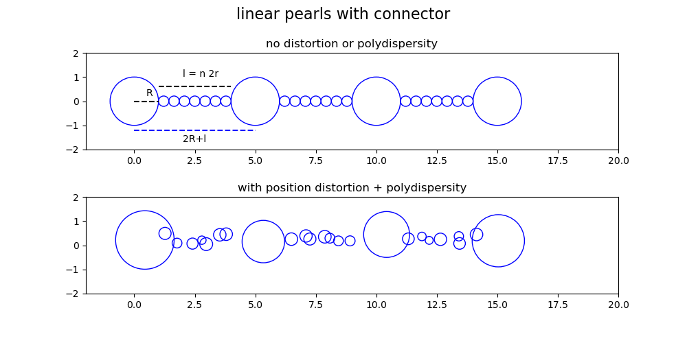
The form factor is \(P(Q)=< F_a(q) \cdot F_a^*(q) >=< |F(q)|^2 >\) We calculate the scattering amplitude \(F_a(q)\) with scattering amplitude \(b_i(q)\)
\[F_a(q)= \sum_N b_i(q) e^{i\mathbf{qr_i}} / \sum_N b_i(q=0)\]Here we use \(b_i(q)\) of spheres (or coreShell) and Gaussians to describe the pearls and linear connectors. Positions are arranged along a line (x axis) with positions \(x_{p=[0..N-1]}=p(2R+2d_{shell}+l)\) for pearls and coils of radius \(r_c=l/(2n)\) at positions
\(x_{p=[0..N-1],c=[0..n-1]}=p(2R+l) + R +d_{shell}+ r_c +c 2r_c\) .
The ensemble average \(<>\) is done as explicit orientational average or using the Debye function. The explicit orientational average allows to include rms and polydispersity with random position and size changes in each step.
The scattering length density in a pearl may include swelling of the pearl material by solvent.
References
For linear pearls without connector
[1]Cascade of Transitions of Polyelectrolytes in Poor Solvents A. V. Dobrynin, M. Rubinstein, S. P. Obukhov Macromolecules 1996, 29, 2974-2979
Linear pearls with polydispersity, pearls in cylinder, NO connectors
[2]Form factor of cylindrical superstructures Leonardo Chiappisi et al. J. Appl. Cryst. (2014). 47, 827–834
Liao uses Simulation to come to a similar formfactor as found here with connectors, rms and polydispersity.
[3]Counterion-correlation-induced attraction and necklace formation in polyelectrolyte solutions: Theory and simulations. Liao, Q., Dobrynin, A. V., & Rubinstein, M. Macromolecules, 39(5), 1920–1938.(2006). https://doi.org/10.1021/ma052086s
Examples
Linear Pearls with position distortion smear out the correlation peak. The smeared out low Q range is similar to [3] Figure 11.
Polydispersity reduces the characteristic minimum and fills the characteristic sphere minimum.
The bumpy low q scattering is due to the random values for rms and polydispersity and vanish for larger values of relError as this increases the number of points in the explicit sphericalaverage. At the same time computing time increases.
import jscatter as js
q=js.loglist(0.02,5,300)
p=js.grace(1.2,1)
for rms in [0.3,1,1.5,2]:
   fq=js.ff.linearPearls(q,N=3,R=2,l=2,pearlSLD=1,cr=0,n=1,relError=200, rms=rms, ffpolydispersity=0)
   p.plot(fq,li=[3,3,-1],sy=0,le=f'rms={rms:.1f}')
for pp in [0.05,0.1,0.2]:
   fq=js.ff.linearPearls(q,N=3,R=2,l=2,pearlSLD=11,cr=0,n=1,relError=200, rms=rms, ffpolydispersity=pp)
   p.plot(fq,li=[1,3,-1],sy=0,le=f'rms={rms:.0f} polydisp={pp:.2f}')
p.yaxis(scale='l',label='I(Q)',min=1e-4,max=1.2)
p.xaxis(scale='l',label='q / nm\S-1',min=0.04,max=7)
p.legend(x=0.05,y=0.01)
p.title('linear pearls with position distortion')
p.subtitle('and polydispersity')
#p.save(js.examples.imagepath+'/linearPearls2.jpg')
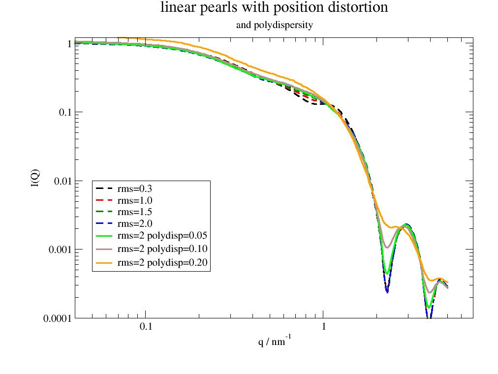
Longer or stronger connector fill up the characteristic sphere minimum.
import jscatter as js
q=js.loglist(0.05,5,300)
p=js.grace(1.5,1)
for n in [0,0.5,1.3,2]:
    fq=js.ff.linearPearls(q,N=5,R=4,l=5,pearlSLD=100,cr=n,n=1)
    p.plot(fq,li=[1,2,-1],le='cr={0:.1f}'.format(n))
p.plot(fq.formfactoramplitude_q,fq.formfactoramplitude[0]**2,le='single sphere')
p.plot(fq.formfactoramplitude_q,fq.formfactoramplitude[1]**2,le='single gaussian')
p.yaxis(scale='l',label='I(Q)',min=0.00001,max=1.1)
p.xaxis(scale='l',label='q / nm\S-1',min=0.05,max=6)
p.legend(x=0.1,y=0.01)
p.title('linear pearls with gaussian connector')
#p.save(js.examples.imagepath+'/linearPearls.jpg')
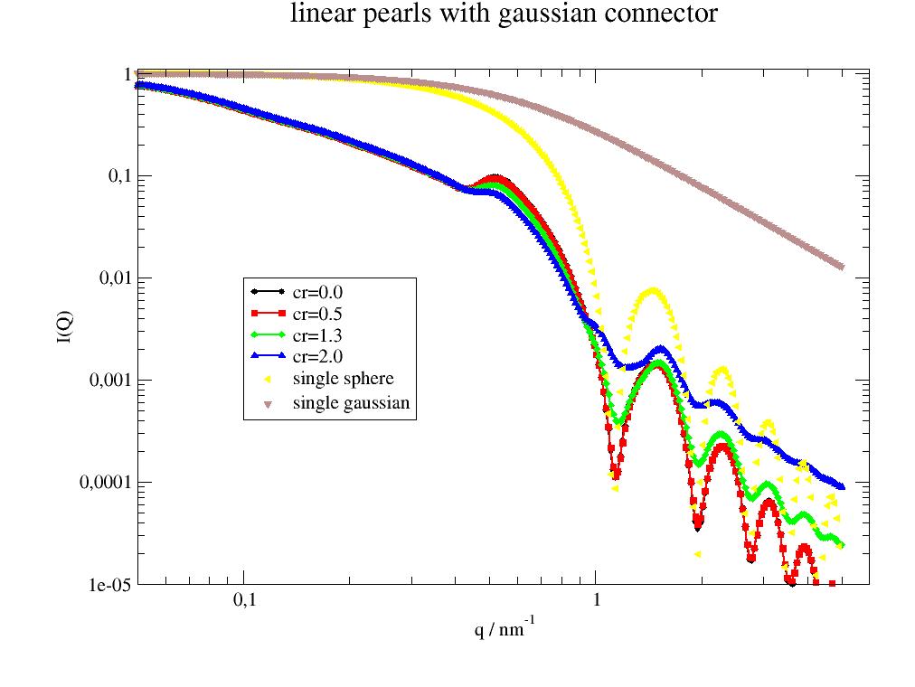
- jscatter.ff.multiArmStarORZ(q, f_arm=4, n_arm=10, l=1, fa=None, costheta=0.0)[source]
Formfactor of a linear polymer chain using optimized Rouse-Zimm approximation (ORZ).
The linear chain is decribed within the more general optimized Rouse-Zimm (ORZ) approximation introduced by Bixon and Zwanzig [3] [4] . See
solveOptimizedRouseZimm().We extend this here using bead scattering lengths for partial matching and allow individual bond correlations.
- Parameters:
- qarray
Scattering vectors in units 1/nm.
- f_armint
Number of arms \(f_{arm}\).
- n_armint
Number of beads per arm \(n_{arm}\) excluding the center common for all arms. Number of beads N is N = f_arm * n_arm + 1
- lfloat, default = 0.38 nm (amino acid)
Bond length or Kuhn length in units nm.
- faNone, list of float
Scattering length of bead/monomer \(fa_i\). Can be used to match parts of the star to the solvent.
None : Equal 1 for all beads.
list: length N as scattering length of beads in sequence
- costhetafloat, list of float, 0 <= costheta < 0.1
Cos of bond correlation angle \(\langle \vec{l_i} \cdot \vec{l_j} \rangle /l^2 = cos(theta)\) between bonds \(l_i\) with \(0 \le cos(\theta) \le 1\).
costheta = 0 : FJC (freely jointed chain) model, no bond correlation, Rouse dynamics, No HI .
float \(0 < cos(\theta) \le 1\) : FRC (free rotating chain). With \(R_{ee} = Nl^2C_{\infty}=Nl^2 \frac{1+cos(\theta)}{1-cos(\theta)}\) .
list of float of length
n_arm-1for the consecutive bonds of an arm. e.gfa=([0.5]*5+[0.1]*6)for stretched inner and flexible outer arms. For the core see below
- e.g. (from [5]_ p. 53) \(C_{\infty} | Kuhn length [A] | cos(theta)\)
polyisoprene 4.6 | 8.2 | 0.783
polyethylene oxide 6.7 | 11 | 0.85
polyethylene 7.4 | 14 | 0.865
atactic polystyrene 9.5 | 18 | 0.895
costheta of the core bonds is \(cos(\theta) = (f_{arm}-1)^{-1}\) to yield a symmetric core. For \(f_{arm}=2\) the core is not special and we use costheta of the innermost bead in an arm to result in a linear chain.
During fits use
limits(costheta=[None,None,0.00,0.999])to avoid singular matrices.
- Returns:
- fqdataArray
Formfactor a linear chain.
[q; fq]
columnname = ‘q;fq’
.costheta : costheta
.l : bondlength l
.N : Number of beads
.Rg : radius of gyration in nm
.Rg_red : reduced radius of gyration
Notes
See
solveOptimizedRouseZimm()for a description of the ORZ model with respective parameters and the form factor \(F(q)\) .Here we use a symetric star with f_arm arms of each n_arm beads and a connecting bead as described by Guenza [1] and set elements \(U^{-1}_{ij} <0.001 \rightarrow 0\).
The inverse of the static bond correlation matrix \(U_{ij}^{-1} = \langle l_i\cdot l_j\rangle /l^2\) in dimesionless form is
\[\begin{split}U_{ij}^{-1} &= \delta_{i,j} &\text{ for uncorrelated bonds } \\\end{split}\]For individual \(g_i\) including that g all are the same and core \(g_0\) (indexing start at 1)
\[\begin{split}U_{ij}^{-1} &= \prod_{n=i}^{j} g_n &\text{ for i,j on the same arm} \\ &= g_0 \prod_{n=1}^{j} g_n \prod_{m=1}^{i} g_m &\text{ for i,j on different arms}\end{split}\]The transfer matrix M is (ignoring the not used \(M_{1i}\)) accordig to [2] :
\[\begin{split}\begin{align} &M_{1,i} &= 1/N &\text{ for }i=1..n_{arm} \\ &M_{i,i} &= 1 &\text{ for }i=2..n_{arm} \\ &M_{i+1,i} &= -1 &\text{ for }i=2..n_{arm},n_{arm}+2..2n_{arm},...,(f_{arm}-1)N+2...f_{arm}n_{arm} \\ &M_{i,1} &= -1 &\text{ for }i=2, n_{arm}+2,2n_{arm}+2,...,(f_{arm}-1)N+2 \\ &M_{i,j} &= 0 &\text{ all others} \end{align}\end{split}\]References
[1]Static and Dynamic Structure Factors for Star Polymers in θ Conditions. Guenza, M. & Perico, A. Macromolecules 26, 4196–4202 (1993). https://doi.org/10.1021/ma00068a020
[2]A Local Approach to the Dynamics of Star Polymers. Guenza, M., Mormino, M. & Perico, A. Macromolecules 24, 6168–6174 (1991). https://doi.org/10.1021/ma00023a018
[3]Theoretical basis for the Rouse‐Zimm model in polymer solution dynamics. Zwanzig, R. The Journal of Chemical Physics 60, 2717–2720 (1974) https://doi.org/10.1063/1.1681433
[4]A hierarchy of models for the dynamics of polymer chains in dilute solution. Perico, A., Ganazzoli, F. & Allegra, G. The Journal of Chemical Physics 87, 3677–3686 (1987). https://doi.org/10.1063/1.452966
Examples
Here we examine how changig stiffness influences the form factor and compare stars with linear chains of same bead number.
import jscatter as js
import numpy as np

q= js.loglist(0.02,5,100)

def stiffendsstar(q, f,n, l=0.5, cosmin =0.05, cosmax=0.8, fa=None):
   costheta = (cosmax-cosmin) * (np.r_[0:1:(n-1)*1j]) + cosmin
   fq = js.ff.multiArmStarORZ(q, f, n, l=0.5, fa = fa, costheta = costheta)
   return fq

p = js.grace()
p.multi(2,1,vgap=0.25)

for c,cs in enumerate(np.r_[0.:0.95:7j],1):
    fq = stiffendsstar(q, 10, 20, l=1, cosmin =0.1, cosmax=cs)
    p[0].plot(fq,li=[1,1,c],sy=0,le=f'cs={cs:.2f} Rg={fq.Rg:.2f} nm\\S-1')
    p[1].plot(fq.X,fq.Y*fq.X**2,li=[1,1,c],sy=0,le=f'Rg={fq.Rg:.2f} nm\\S-1')

for c,cs in enumerate(np.r_[0.:0.95:7j],1):
    fq = stiffendsstar(q, 2, 5*20, l=1, cosmin =0.1, cosmax=cs)
    p[0].plot(fq,li=[3,1,c],sy=0,le=f'cs={cs:.2f} Rg={fq.Rg:.2f} nm\\S-1')
    p[1].plot(fq.X,fq.Y*fq.X**2,li=[3,1,c],sy=0,le=f'Rg={fq.Rg:.2f} nm\\S-1')

# a matched star core pronounces the linear ends
fa= [0]+([0]*10+[1]*10)*10
fq = stiffendsstar(q, 10, 20, l=1, cosmin =0.1, cosmax=cs,fa=fa)
p[0].plot(fq,li=[1,1,c],sy=0,le=f'matched core ')
p[1].plot(fq.X,fq.Y*fq.X**2,li=[1,1,c],sy=0,le=f'Rg={fq.Rg:.2f} nm\\S-1')

p[0].xaxis(label=r'Q / nm\S-1',scale='log')
p[1].xaxis(label=r'Q / nm\S-1',min=0,max=3)
p[0].yaxis(label=r'I(Q)',scale='log',min=100,max=1e5)
p[1].yaxis(label=r'I(Q)Q\S2',scale='norm',min=0.0,max=4000)
p[0].text('matched core',x=0.02,y=7000)
p[0].text(r'Q\S-1\N => linear chains',x=0.5,y=400,rot=340,charsize=0.7)
p[1].text(r'Q\S-1\N => linear chains',x=2,y=1200,rot=12,charsize=0.7)

p.title('stars and linear chains with stiff ends')
p.subtitle('stars: solid lines; linear chains broken lines')
p[0].legend(x=3,y=2e5,charsize=0.4)
# p.save(js.examples.imagepath+'/ORZ_starstiffends_ff.png',size=(1.5,1.5),dpi=300)
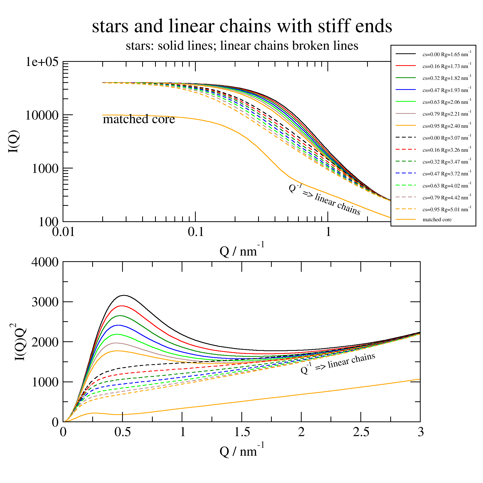
- jscatter.ff.multiShellBicelle(q, R, shellthickness, shellSLD, dR=None, p=1, rimthickness=None, rimSLD=None, solventSLD=0, alpha=None, n=17)[source]
Multi shell bicelle as flat disc with curved rim in solvent.
Head and tails of lipids need at least a core (tails) and an outer shell (heads).
- Parameters:
- qarray
Wavevectors, units 1/nm.
- Rfloat
Radius of the disc core without the rim part in units nm.
- dRfloat, default 1% of R
1-Sigma width of a radius distribution in units nm.
- shellthicknesslist of float or float, all >=0
Thickness of disc shells from inner to outer along disc axis, units nm, same shape as radialthickness. \(D_i = \sum_{j=1}^i shellthickness_j\)
Innermost thickness is doubled (core counted as 2 shells on both sides from zero).
total thickness = 2 * cumulativeSum(shellthickness)
- rimthicknesslist of float or float like shellthickness, all >0 or None
Thickness of rim shells at equator from inner to outer, units nm. \(R_i = \sum_{j=1}^i rimthickness_j\)
If None same as shellthickkness
For zero rimthickness a shell vanishes at the equator but continues to the edge of the disc. Only if all inner shells are zero we get the picture of the last sketch below.
rimthickness_i can be larger as shellthickness_i
The rim continues to the shell edge.
- pfloat, default=1
Parameter that describes the rim shape (see
superball()).The rim shell edges are described by \(x^{2p} = R_i^{2p}(1- (z/D)^{2p})\) using \((x/R_i)^{2p} - (z/D_i)^{2p}) =1\) with rim outer radius R at height z. This creates a continuous transition in shells.
p=1 : circle like
1<p<2 : rounded rectangular
p>5 : approaches rectangular shape
p<1 convex
p=0.5 : linear (not for bicelles)
- shellSLDlist of float/list
Scattering length density of disc shells up to radius R in nm^-2. A shell can be divided in sub shells if instead of a single float a list of floats is given. These list values are used as scattering length of equal thickness subshells. E.g. [1,2,[3,2,1]] results in the last shell with 3 subshell of equal thickness. The sum of subshell thickness is the thickness given in shellthickness. See second example. SiO2 = 4.186*1e-6 A^-2 = 4.186*1e-4 nm^-2
- rimSLDlist of float/list
Scattering length density of shells in the rim in nm^-2. If None its the same as the shellSLD.
- solventSLDfloat
Scattering length density of surrounding solvent in nm^-2. D2O = 6.335*1e-6 A^-2 = 6.335*1e-4 nm^-2
- alphafloat, [float,float] , unit rad, default [0,π/2]
Orientation, angle between the cylinder axis and the scattering vector q. 0 means parallel, pi/2 is perpendicular If alpha =[start,end] is integrated between start,end start > 0, end < pi/2
- nint, default 17
Number of points in Gauss integration along alpha and R distribution.
- Returns:
- dataArray
- Columns [q ,Iq ]
.outerDiscVolume
.radii
.alpha
.discthickness
.rimthickness
.R
.shellSLD
.rimSLD
.solventSLD
.modelname
Examples
Different bicelles for p=1. Colors code SLD.

A bicelle model with an interfacial layer as example how to fit bicelles.
The model can be extended by different scattering length densities for rim or other things that might be important e.g. if tails differ in disc and rim.
The difference ins SLD is strongly correlated to the scaling ‘A’. If A, shead and stail are fitted the errors are huge because of the correlation. Best is to fix e.g. stail.
import jscatter as js
import numpy as np

bi0 = js.dA(js.examples.datapath + '/bicelleDMPC-DHCP_5mg.csv', replace={',': ' '})


def bi(q, R, dR, tail, head, stail=290, shead=420, p=1, A=1, bgr=0, di=0.1):
    # bicelle model with an interface between tail/head and head/solvent
    # tail, head : float , thickness of layer
    # shead, stail : float SDL of layer in electron density unis (e/nm^3)
    sld = np.r_[stail, shead] * js.formel.felectron  # DPPC SAXS
    rim = np.r_[tail, head]
    solventSLD = 334 * js.formel.felectron
    # tail, head layers with interface regions of dd thickness
    sldp = np.r_[stail, (stail + shead) / 2, shead, (shead + solventSLD) / 2] * js.formel.felectron

    bicelle = js.ff.multiShellBicelle(q, R=R, shellthickness=[tail, di, head, di],
                                      rimthickness=[tail, di, head, di],
                                      p=p, dR=dR, shellSLD=sldp, rimSLD=sldp, solventSLD=solventSLD)

    # add background and scaling
    bicelle.Y = A * bicelle.Y + bgr
    return bicelle


free0 = {'R': 1.58, 'tail': 1.47, 'head': 0.37, 'shead': 460, 'stail': 292, 'A': 1933, 'bgr': 0.0001, 'dR': 0.5}
fix = {'p': 1, 'di': 0.1}
free = free0.copy()

#bi0.eY[bi0.X>0.89] *= 2
bi0.makeErrPlot(xscale='log', yscale='log')
bi0.setlimit(head=[0, 1.5], tail=[0, 3], R=[1, 6], shead=[350, 540], stail=[250, 320], dR=[0, 0.7], bgr=[0, 0.002],
             A=[0, None, 0])

bi0.setlimit(p=[1, 5, 0.99], hr=[0, 1])
bi0.fit(bi, free, fix, {'q': 'X'}, condition=lambda a: a.X > 0.3),  # method='diff',workers=12)
bi0.errPlotTitle(bi0.name.split('/')[-1].split('.')[0])
bi0.errplot.legend(x=1,y=0.002)

# bi0.savelastErrPlot(js.examples.imagepath+'/interfacialBicelle.jpg',size=[2,2])
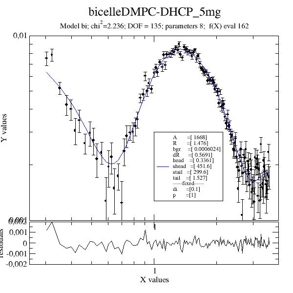
Nearly Contrast matched bicelle in SAXS. Example data for DPPC lipid with DHCP rim. DPPC liposomes show a suppressed forward scattering in SAXS as the contrast releative to surrounding water has opposite sign (see DPPC Vesicle in SAXS).
The more curved rim changes the matching condition (\(\rho_{tails}^2V_{tails}^2 \approx \rho_{head}^2V_{head}^2\)) and thereby changing the relation between \(I_0\) and the peak max.
import jscatter as js
import numpy as np
Q = js.loglist(0.01,5,400)

# bicelle with tails and heads
sld = np.r_[290, 420] * js.formel.felectron # DPPC SAXS
solventSLD = 334 * js.formel.felectron
rim = [1.5, 0.5]
R = 2

p = js.grace()
for c,pp in enumerate([1,2,5],1):
    bicelle = js.ff.multiShellBicelle(Q, R=R,shellthickness=rim, rimthickness=rim,p=pp,dR=0.1,
                                           shellSLD=sld,solventSLD=solventSLD)
    p.plot(bicelle.X,bicelle.Y/bicelle.I0,sy=0,li=[1,3,c], le=f'bicelle p={pp:.1f}')

# rectangular bicelle
rbicelle = js.ff.multiShellDisc(Q,radialthickness=[R+rim[0],rim[1]],shellthickness=rim,
               shellSLD=sld,solventSLD=solventSLD)
p.plot(rbicelle.X,rbicelle.Y/rbicelle.I0, sy=0,li=[3,2,2], le='rectangular bicelle')

p.yaxis(label=r'I(q)',scale='l',min=0.005,max=1)
p.xaxis(label=r'q / nm\S-1',scale='l',min=0.01,max=5)
p.legend(x=0.02,y=0.04)
p.title('SAXS bicelle')
# p.save(js.examples.imagepath+'/multiShellBicelle.jpg')
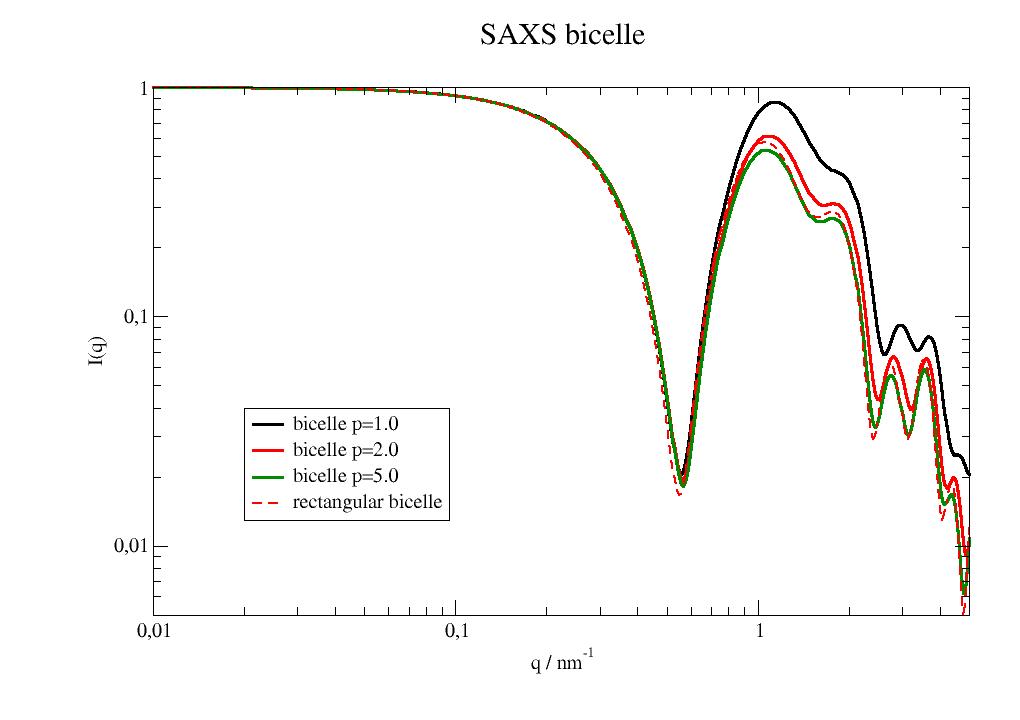
- jscatter.ff.multiShellCylinder(q, L, shellthickness, shellSLD, solventSLD=0, alpha=None, h=None, nalpha=60, ncap=31)[source]
Multi shell cylinder with caps in solvent averaged over axis orientations.
Each shell has a constant SLD and may have a cap with same SLD sequence. Caps may be globular (barbell) or small (like lenses). For zero length L a lens shaped disc or a double sphere like shape is recovered.
The models in the references are extended to multiple shells. This allows to approximate continuous profiles by step profiles with large number of shells.
- Parameters:
- qarray
Wavevectors, units 1/nm
- Lfloat
Length of cylinder, units nm L=0 infinite cylinder if h=None.
- shellthicknesslist of float or float, all >0
Thickness of shells in sequence, units nm. radii R = cumulativeSum(shellthickness)
- shellSLDlist of float/list
Scattering length density \(\rho_{i}\) of shells in nm^-2. A shell can be divided in sub shells if instead of a single float a list of floats is given. These list values are used as scattering length of equal thickness subshells. E.g. [1,2,[3,2,1]] results in the last shell with 3 subshell of equal thickness. The sum of subshell thickness is the thickness given in shellthickness. See second example. SiO2 = 4.186*1e-6 A^-2 = 4.186*1e-4 nm^-2
- solventSLDfloat
Scattering length density \(\rho_{sol}\) of surrounding solvent in nm^-2. D2O = 6.335*1e-6 A^-2 = 6.335*1e-4 nm^-2
- hfloat, default=None
Geometry of the caps with cap radii R=(r**2+h**2)**0.5 h is distance of cap center with radius R from the flat cylinder cap and r as radii of the cylinder shells.
None No caps, flat ends as default.
0 cap radii equal cylinder radii (same shellthickness as cylinder shells)
>0 cap radius larger cylinder radii as barbell
<0 cap radius smaller cylinder radii as lens caps
- alphafloat, [float,float] , unit rad
Orientation, angle \(\alpha\) between the cylinder axis and the scattering vector q. 0 means parallel, pi/2 is perpendicular If alpha =[start,end] is integrated between start,end start > 0, end < pi/2
- nalphaint, default 30
Number of points in Gauss integration along alpha.
- ncapint, default=31
Number of points in Gauss integration for cap.
- Returns:
- dataArray
- Columns [q ,Iq ]
.outerCylinderVolume
.Radius
.cylinderLength
.alpha
.shellthickness
.shellSLD
.solventSLD
.modelname
.contrastprofile
.capRadii
Notes
Formfactor F(q) of multishell cylinder (L>R) or disc (L<R) with contrast \(\Delta=(\rho_{cyl,i}-\rho_{sol})\) and optional cap/barbell
\[F(q) = \int_0^{\pi/2} f_a^2(q,\alpha) sin(\alpha) d\alpha\]\[f(q,\alpha) = \sum_{i=1}^n [f_a^i(q,\alpha,\Delta_i) - f_a^{i-1}(q,\alpha,\Delta_{i-1})]\]subtracting the inner cylinders with \(f_a^0(...) = 0\) and cylinders formfactor amplitudes
\[f_a^i(q,\alpha,\Delta_i) = \Delta \pi R_i^2 L_i j_0(qcos(\alpha)L_i/2) \frac{J_1(qR_isin(\alpha))}{qR_isin(\alpha)}\]with \(j_0=sin(x)/x\) and \(J_1(x)\) as first order Bessel function. Nested shells i=1..n with n=1 for single cylinder.
Cap/barbell on cylinder bottom and top with cap radius \(R_c\) and cap center at h from cylinder top [5].
\[\begin{split}f_{a,cap} (q,\alpha,\Delta_c) = 4\pi R_c^3 \int_{-h/R}^1 dt & cos[q cos(\alpha) (Rt+h+L/2)] \\ & \times (1-t^2) \frac{J_1[qRsin(\alpha)(1-t^2)^{1/2}]}{qRsin(\alpha)(1-t^2)^{1/2}}\end{split}\]and \(f_a^i(q,\alpha,\Delta_i) \Rightarrow f_a^i(q,\alpha,\Delta_i) + f_{a,cap}^i (q,\alpha,\Delta_c^i)\)
Multishell cylinders types:
flat cap
L>0, radii>0, h=None
lens cap
L>0, radii>0, h<0
lens cap, R=r
L>0, radii>0, h=0
barbell, globular cap
L>0, radii>0, h>0
lens, no cylinder
L=0, radii>0, h<0
barbell, no cylinder
L=0, radii>0, h>0
infinite flat disc
L=0. h=None
Compared to SASview this yields a factor 2 less. See
cylinder()References
Single cylinder
[1]Guinier, A. and G. Fournet, “Small-Angle Scattering of X-Rays”, John Wiley and Sons, New York, (1955)
Double cylinder
[3]Use of viscous shear alignment to study anisotropic micellar structure by small-angle neutron scattering, J. B. Hayter and J. Penfold J. Phys. Chem., 88:4589–4593, 1984
Barbell, cylinder with small end-caps, circular lens
[5]Scattering from cylinders with globular end-caps Kaya (2004). J. Appl. Cryst. 37, 223-230] DOI: 10.1107/S0021889804000020 Scattering from capped cylinders. Addendum H. Kaya and Nicolas-Raphael de Souza J. Appl. Cryst. (2004). 37, 508-509 DOI: 10.1107/S0021889804005709
Examples
Alternating shells with different thickness 0.3 nm h2o and 0.2 nm d2o in vacuum:
import jscatter as js
import numpy as np
x=np.r_[0.0:10:0.01]
ashell=js.ff.multiShellCylinder(x,20,[0.4,0.6]*5,[-0.56e-4,6.39e-4]*5)
#plot it
p=js.grace()
p.new_graph(xmin=0.24,xmax=0.5,ymin=0.2,ymax=0.5)
p[0].plot(ashell)
p[0].yaxis(label='I(q)',scale='l',min=1e-7,max=1)
p[0].xaxis(label='q / nm\S-1',scale='l',min=0.05,max=10)
p[1].plot(ashell.contrastprofile,li=1) # a contour of the SLDs
p[1].subtitle('contrastprofile')
p[0].title('alternating shells')
#p.save(js.examples.imagepath+'/multiShellCylinder.jpg')
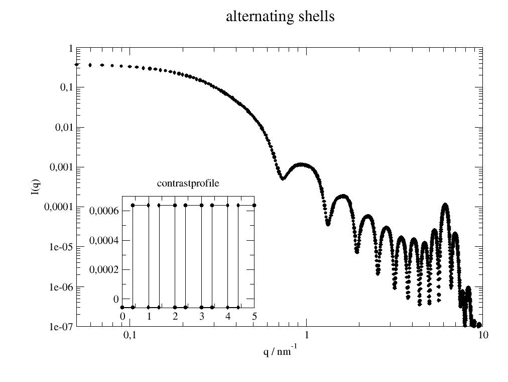
Double shell with exponential decreasing exterior shell to solvent scattering. Details of outer shell are difficult to access.
import jscatter as js
import numpy as np
x=np.r_[0.0:10:0.01]

def doubleexpshells(q,L,d1,d2,e3,sd1,sd2,sol,n=10):
   # The third layer will have n subshells with combined thickness of e3.
   # The scattering length decays to e**(-3) in last subshell.
   return js.ff.multiShellCylinder(q,L,[d1,d2,e3],[sd1,sd2,((sd2-sol)*np.exp(-np.r_[0:3:n*1j])+sol)],solventSLD=sol)

# plot it
p=js.grace()
p.multi(2,1,vgap=0.3)

dde10 = doubleexpshells(x,10,0.5,0.5,3,1e-4,2e-4,0,n=10)
p[0].plot(dde10,sy=[1,0.1,1])
p[1].plot(dde10.contrastprofile,li=1) # a contour of the SLDs

dde50 = doubleexpshells(x,10,0.5,0.65,3,1e-4,2e-4,0,n=50)
p[0].plot(dde50,sy=[1,0.1,2])
p[1].plot(dde50.contrastprofile,sy=[1,0.1,2],li=1) # a contour of the SLDs

p[0].yaxis(label='I(q)',scale='l',min=1e-10,max=0.001)
p[0].xaxis(label='q / nm',scale='n')
p[1].yaxis(label='sld(r)',min=0,max=0.00025)
p[1].xaxis(label='r / nm',scale='n')
p[1].text('scattering length profile',x=2,y=0.00017)
p[0].title('Double shell with exponential decreasing exterior shell')
# p.save(js.examples.imagepath+'/multiShellCylinder_exp.jpg')
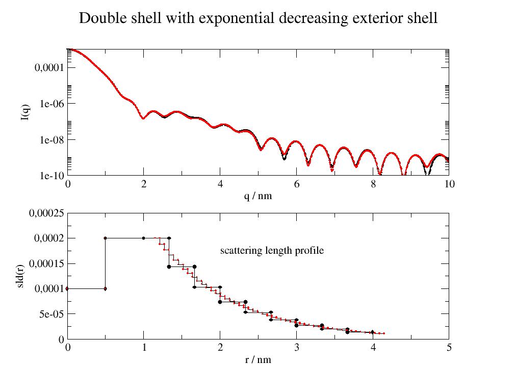
Cylinder with cap:
x=np.r_[0.1:10:0.01]
p=js.grace()
p.title('Comparison of dumbbell cylinder with simple models')
p.subtitle('thin lines correspond to simple models as sphere and dshell sphere')
p.plot(js.ff.multiShellCylinder(x,0,[10],[1],h=0),sy=[1,0.5,2],le='simple sphere')
p.plot(js.ff.sphere(x,10),sy=0,li=1)
p.plot(js.ff.multiShellCylinder(x,0,[2,1],[1,2],h=0),sy=[1,0.5,3],le='double shell sphere')
p.plot(js.ff.multiShellSphere(x,[2,1],[1,2]),sy=0,li=1)
p.plot(js.ff.multiShellCylinder(x,10,[3],[20],h=-5),sy=[1,0.5,4],le='thin lens cap cylinder=flat cap cylinder')
p.plot(js.ff.multiShellCylinder(x,10,[3],[20],h=None),sy=0,li=[1,2,1],le='flat cap cylinder')
p.plot(js.ff.multiShellCylinder(x,10,[3],[20],h=-0.5),sy=0,li=[3,2,6],le='thick lens cap cylinder')
p.yaxis(scale='l')
p.xaxis(scale='l')
p.legend(x=0.15,y=0.01)
- jscatter.ff.multiShellDisc(q, radialthickness, shellthickness, shellSLD, solventSLD=0, alpha=None, nalpha=60)[source]
Multi shell disc (e.g. bicelle) in solvent averaged over axis orientations.
Disc models for discs, multidiscs (e.g. cheese burger), bicelle, multishell bicelle and more. For bicelles this is the rectangular core shell model often used for bicelles.
- Parameters:
- qarray
Wavevectors, units 1/nm.
- radialthicknessfloat, all >0
- Radial thickness of disc shells from inner to outer, first corresponds to core radius, units nm.
outer radius R = cumulativeSum(radialthickness)
Zero outer shells allow to make disc stacks without overlapping border.
- shellthicknesslist of float or float, all >=0
- Thickness of shells from inner to outer along disc axis, units nm.
Same length as radialthickness.
Innermost thickness is doubled (core counted as 2 shells on both sides from zero).
total thickness = 2*cumulativeSum(shellthickness)
For shellthickness =0 a infinitely thin disc is returned. The forward scattering I0 needs to be multiplied by a length to have conventional units.
- shellSLDlist of float/list
Scattering length density of shells in nm^-2. A shell can be divided in sub shells if instead of a single float a list of floats is given. These list values are used as scattering length of equal thickness subshells. E.g. [1,2,[3,2,1]] results in the last shell with 3 subshell of equal thickness. The sum of subshell thickness is the thickness given in shellthickness. See second example. SiO2 = 4.186*1e-6 A^-2 = 4.186*1e-4 nm^-2
- solventSLDfloat
Scattering length density of surrounding solvent in nm^-2. D2O = 6.335*1e-6 A^-2 = 6.335*1e-4 nm^-2
- alphafloat, [float,float] , unit rad
Orientation, angle between the cylinder axis and the scattering vector q. 0 means parallel, pi/2 is perpendicular If alpha =[start,end] is integrated between start,end start > 0, end < pi/2
- nalphaint, default 30
Number of points in Gauss integration along alpha.
- Returns:
- dataArray
- Columns [q ,Iq ]
.outerDiscVolume
.radii
.alpha
.discthickness
.shellSLD
.solventSLD
.modelname
Notes
The model is the same as for
multiShellCylinder()except that the cylinder length is also changing with shellthickness.References
[1]Guinier, A. and G. Fournet, “Small-Angle Scattering of X-Rays”, John Wiley and Sons, New York, (1955)
[2] (1,2)Dos Santos Morais et al Contrast-Matched Isotropic Bicelles: A Versatile Tool to Specifically Probe the Solution Structure of Peripheral Membrane Proteins Using SANS Langmuir 2017, 33, 26, 6572–6580, https://doi.org/10.1021/acs.langmuir.7b01369
Examples
Different discs :
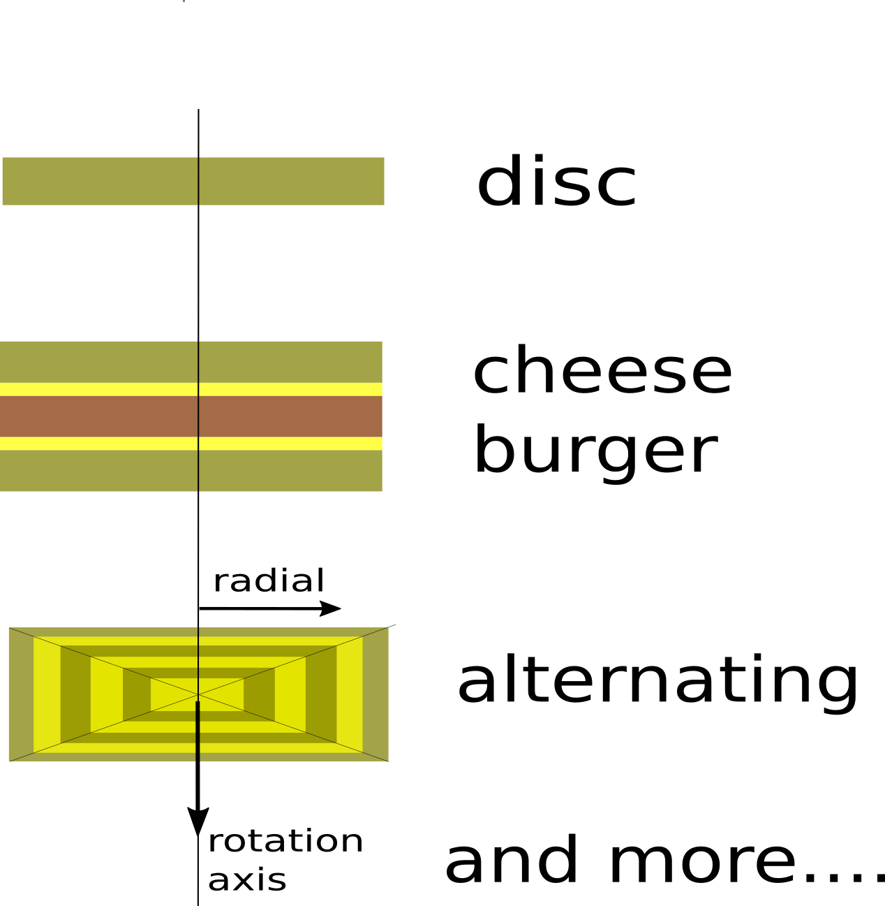
import jscatter as js
import numpy as np
x=np.r_[0.0:10:0.01]
p=js.grace()

# single disc
bshell = js.ff.multiShellDisc(x,2,2,6.39e-4)
p[0].plot(bshell, le='disc')

# Cheese burger with double cheese, patty and cheese are visible (zeros in radialthickness)
cheese = js.ff.multiShellDisc(x,[5,0,0],[1,0.2,2],np.r_[3,2,1]*1e-4)
p[0].plot(cheese, le='cheese')

# alternating shells
ashell = js.ff.multiShellDisc(x,[0.6,0.4]*2,[0.4,0.6]*2,[-0.56e-4,6.39e-4]*2)
p[0].plot(ashell, le='alternating')

p[0].yaxis(label='I(q)',scale='l',min=1e-7,max=0.01)
p[0].xaxis(label='q / nm\S-1',scale='l',min=0.1,max=10)
p[0].legend(x=2,y=0.003)
p[0].title('multishell discs')
#p.save(js.examples.imagepath+'/multiShellDisc.jpg')
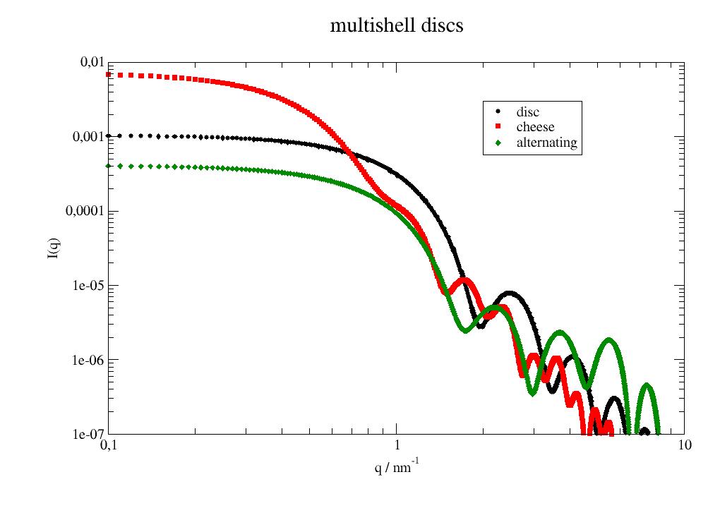
Contrast matched bicelle in SANS (see [2] for details). In [2] no smearing was applied to the model as it should for SANS. The scattering of a single bicelle (core shell model) is calculated.
import jscatter as js
import numpy as np

q=np.r_[0.0:4:0.01]
head = 0.6
rim = 1.1  # nm, rim thickness => DHPC length
th = 2.0  # nm, flat half bicelle thickness => DMPC length
R = 4.2  #  nm, outer radius of core = DMPC radius + rim

hsld = np.r_[-0.58,2.24]*1e-4  # scattering length densities
hbicelle = js.ff.multiShellDisc(q, radialthickness=[R,head], shellthickness=[th-head,head],
                                                shellSLD=hsld, solventSLD=6.335*1e-4)

dsld = np.r_[7.39,5.05]*1e-4  # scattering length densities full deuteration
dbicelle = js.ff.multiShellDisc(q, radialthickness=[R,head], shellthickness=[th-head,head],
                                                shellSLD=dsld,solventSLD=6.335*1e-4)

dsld67 = np.r_[6.65,6.65]*1e-4  # scattering length densities DMPC d67
dbicelle67 = js.ff.multiShellDisc(q, radialthickness=[R,head], shellthickness=[th-head,head],
                                                shellSLD=dsld67,solventSLD=6.335*1e-4)
p=js.grace()
p.plot(hbicelle, le='h-bicelle')
p.plot(dbicelle, le='d-bicelle')
p.plot(dbicelle67, le='d67-bicelle')

p.yaxis(label='I(q)',scale='l',min=1e-7,max=0.01)
p.xaxis(label='q / nm\S-1',scale='l',min=0.1,max=10)
p.title('Bicelle SANS scattering (no smearing)')
p.legend(x=2,y=0.003)
#p.save(js.examples.imagepath+'/bicelleSANS_multishell.jpg')
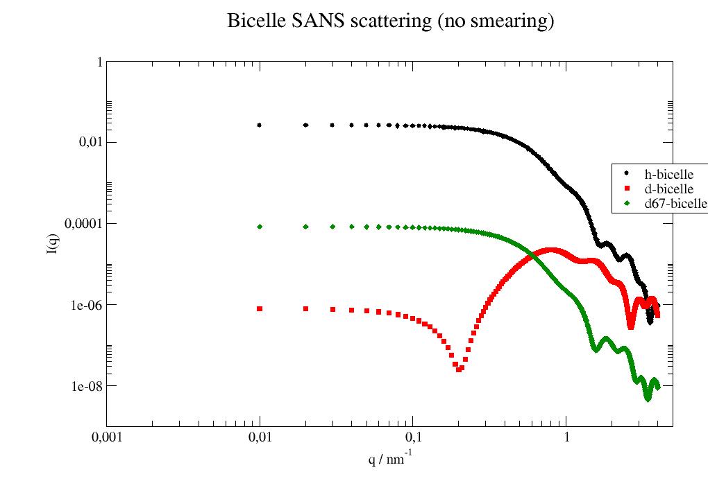
- jscatter.ff.multiShellEllipsoid(q, poleshells, equatorshells, shellSLD, solventSLD=0, alpha=None, tol=1e-06)[source]
Scattering of multi shell ellipsoidal particle with varying shell thickness at pole and equator.
Shell thicknesses add up to form complex particles with any combination of axial ratios and shell thickness. A const axial ratio means different shell thickness at equator and pole.
- Parameters:
- qarray
Wavevectors, unit 1/nm
- equatorshellslist of float
Thickness of shells starting from inner most for rotated axis Re making the equator. unit nm. The absolute values are used.
- poleshellslist of float
Thickness of shells starting from inner most for rotating axis Rp pointing to pole. unit nm. The absolute values are used.
- shellSLDlist of float
List of scattering length densities of the shells in sequence corresponding to shellthickness. unit nm^-2.
- solventSLDfloat, default=0
Scattering length density of the surrounding solvent. unit nm^-2
- alpha[float,float], default [0,90]
Angular range of rotated axis to average over in degree. Default is no preferred orientation.
- tolfloat
Absolute tolerance for above adaptive integration of alpha.
- Returns:
- dataArray
- Columns[q, Iq, beta]
- Iq scattering cross section in units nm**2
.contrastprofile as radius and contrast values at edge points of equatorshells
.equatorshellthicknes consecutive shell thickness
.poleshellthickness
.shellcontrast contrast of the shells to the solvent
.equatorshellradii outer radius of the shells
.poleshellradii
.outerVolume Volume of complete sphere
.I0 forward scattering for Q=0
.alpha integration range alpha
References
[1]Structure Analysis by Small-Angle X-Ray and Neutron Scattering Feigin, L. A, and D. I. Svergun, Plenum Press, New York, (1987).
[3]Kotlarchyk and S.-H. Chen, J. Chem. Phys. 79, 2461 (1983).
Examples
Simple ellipsoid in vacuum:
import jscatter as js
import numpy as np
q=np.r_[0.0:10:0.01]
Rp=2.
Re=1.
ashell=js.ff.multiShellEllipsoid(q,Rp,Re,1)
#plot it
p=js.grace()
p.multi(2,1)
p[0].plot(ashell)
p[1].plot(ashell.contrastprofile,li=1) # a contour of the SLDs
Core shell ellipsoid with a spherical core
Dependent on shell thickness at pole or equator the shape is oblate or prolate with a spherical core.
import jscatter as js
import numpy as np
q=np.r_[0.0:10:0.01]
def coreShellEllipsoid(q,Rcore,Spole,Sequ,bc,bs):
    ellipsoid = js.ff.multiShellEllipsoid(q,[Rcore,Spole],[Rcore,Sequ],[bc,bs])
    return ellipsoid

p=js.grace()
p.multi(2,1,vgap=0.25)
for eq in [0.1,1,2]:
    ell = coreShellEllipsoid(q,2,1,eq,1,2)
    p[0].plot(ell)
    p[1].plot(ell.contrastprofile,li=1) # a contour of the SLDs
p[0].yaxis(label='I(q)',scale='log')
p[0].xaxis(label='q / nm\S-1')
p[1].yaxis(min=0,max=3)
p[1].xaxis(label='radius / nm')
Alternating shells with thickness 0.3 nm h2o and 0.2 nm d2o in vacuum:
import jscatter as js
import numpy as np
x=np.r_[0.1:10:0.01]
shell=np.r_[[0.3,0.2]*3]
sld=[-0.56e-4,6.39e-4]*3

# constant axial ratio for all shells but non constant shell thickness
axialratio=2
ashell=js.ff.multiShellEllipsoid(x,axialratio*shell,shell,sld)

# shell with constant shellthickness of one component and other const axialratio
pshell=shell[:]
pshell[0]=shell[0]*axialratio
pshell[2]=shell[2]*axialratio
pshell[4]=shell[4]*axialratio
bshell=js.ff.multiShellEllipsoid(x,pshell,shell,sld)

#plot it
p=js.grace()
p.new_graph(xmin=0.24,xmax=0.5,ymin=0.2,ymax=0.5)
p[1].subtitle('contrastprofile')
p[0].plot(ashell,le='const. axial ratio')
p[1].plot(ashell.contrastprofile,li=2) # a contour of the SLDs
p[0].plot(bshell,le='const shell thickness')
p[1].plot(bshell.contrastprofile,li=2) # a contour of the SLDs
p[0].yaxis(scale='l',label='I(q)',min=1e-9,max=0.0002)
p[0].xaxis(scale='l',label='q / nm\S-1')
p[0].legend(x=0.12,y=1e-5)
p[0].title('multi shell ellipsoids')
#p.save(js.examples.imagepath+'/multiShellEllipsoid.jpg')
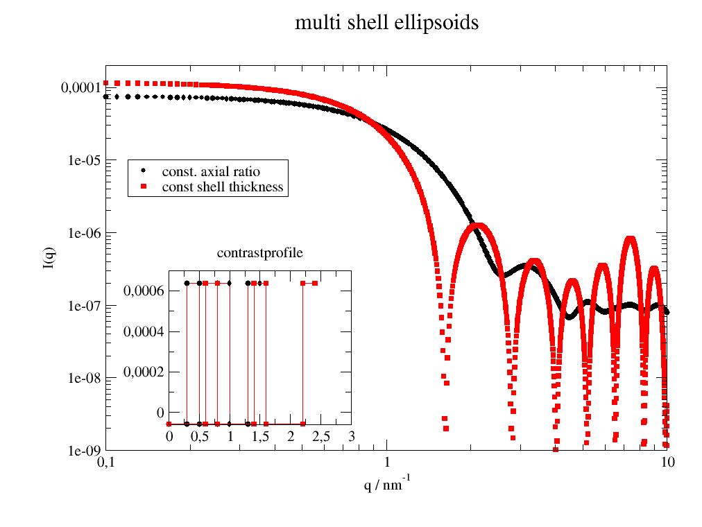
Double shell with exponential decreasing exterior shell
With multiple shells for the exponential outer part. This is described by a single additional parameter. Increasing the number of shells (n) improves the approximation. A lower number is faster and may be a good enough approximation.
import jscatter as js
import numpy as np
x=np.r_[0.0:10:0.01]
def doubleexpshells(q,d1,ax,d2,e3,sd1,sd2,sol,n=9):
   # e3 is 1/e width of the exponential
   # n determines number of shells to approximate exp, we want to calc up to 3*e3
   e3e = e3/n*3  # shell width
   shells =[d1   ,d2] + [e3e/2] + [e3e] * (n-1)
   shellsp=[d1*ax,d2] + [e3e/2] + [e3e] * (n-1)
   sld=[sd1,sd2]+list(((sd2-sol)*np.exp(-np.r_[0:n]*e3e)))
   return js.ff.multiShellEllipsoid(q,shellsp,shells,sld,solventSLD=sol)

#plot it
p=js.grace()
p.multi(2,1,vgap=0.3)
for n in [9,19,29]:
    dde=doubleexpshells(q=x,d1=0.5,ax=1,d2=0.5,e3=1,sd1=1e-4,sd2=2e-4,sol=0,n=n)
    p[0].plot(dde,sy=[1,0.3,-1],le=f'n={n}')
    p[1].plot(dde.contrastprofile,li=1) # a countour of the SLDs

p[0].legend(x=0.2,y=1e-6)
p[0].yaxis(label='F(q)',scale='log',min=1e-11,max=1e-3,ticklabel='power')
p[0].xaxis(label='q / nm\S-1',scale='log',min=0.1,max=10)
p[1].yaxis(label='density * 10\S-4',min=0,max=0.00025,formula='$t*1e4')
p[1].xaxis(label='radius / nm')
p[1].text('approximate density profile',x=2,y=0.0002)
p[0].title('Double shell with exponential decreasing exterior')
#p.save(js.examples.imagepath+'/multiShellEllipsoidExp.jpg')
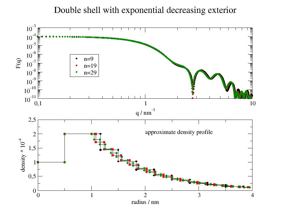
- jscatter.ff.multiShellSphere(q, shellthickness, shellSLD, solventSLD=0)[source]
Scattering of spherical multi shell particle including linear contrast variation in subshells.
The results needs to be multiplied with the concentration to get the measured scattering. The resulting contrastprofile can be accessed as .contrastprofile
- Parameters:
- qarray
Wavevectors to calculate form factor, unit e.g. 1/nm.
- shellthicknesslist of float
Thickness of shells starting from inner most, unit in nm. There is no limit for the number of shells.
- shellSLDlist of float or list
- List of scattering length densities of the shells in sequence corresponding to shellthickness. unit in nm**-2
Innermost shell needs to be constant shell.
If an element of the list is itself a list of SLD values it is interpreted as equal thick subshells with linear progress between SLD values in sum giving shellthickness. Here any shape can be approximated as sequence of linear pieces.
If subshell list has only one float e.g. [1e.4] the second value is the SLD of the following shell.
If empty list is given as [] the SLD of the previous and following shells are used as smooth transition.
- solventSLDfloat, default=0
Scattering length density of the surrounding solvent. If equal to zero (default) then in profile the contrast is given. Unit in 1/nm**2
- Returns:
- dataArray
Columns [wavevector, Iq, Fa] Iq scattering cross section in units nm**2
Fa formfactor amplitude
.contrastprofile as radius and contrast values at edge points
.shellthickness consecutive shell thickness
.shellcontrast contrast of the shells to the solvent
.shellradii outer radius of the shells
.slopes slope of linear increase of each shell
.outerVolume Volume of complete sphere
.I0 forward scattering for Q=0
.fa0 forward scattering amplitude for Q=0
Notes
The scattering intensity for a multishell particle with several subshells is
\[I(q) = F^2_a(q) = \left( \sum_i f_a(q) \right)^2\]The scattering amplitude of a subshell with inner and outer radius \(R_{i,o}\) is
\[f_a(q) = 4\pi\int_{R_i}^{R_o} \rho(r) \frac{sin(qr)}{qr}r^2dr\]where we use always the scattering length density difference to the solvent (contrast) \(\rho(r) = \hat{\rho}(r) - \hat{\rho}_{solvent}\).
For constant scattering length density \(\rho(r) = \rho\) we get
\[f_{a,const}(q) = \frac{4\pi}{3}r^3\rho \left. \frac{3(sin(qr)-qR cos(qr))}{(qr)^3}\right\rvert_{r=R_i}^{r=R_o}\]with forward scattering contribution
\[f_{a,const}(q=0) = \frac{4\pi\rho}{3} (R_i^{3} - R_o^{3})\]For a linear variation as \(\rho(r)=\Delta\rho(r-R_i)/d + \rho_i\) with \(\Delta\rho=\rho_o-\rho_i\) and thickness \(d=(R_o-R_i)\) we may sum a constant subshell as above with \(\rho(r)=\rho_i\) and contribution of the linear increase \(\rho(r)=\Delta\rho(r-R_i)/d\) resulting in
\[f_{a,lin}(q) =f_{a,const}(q) + \frac{4\pi\Delta\rho}{d} \left. \frac{(q(2r-R_i))sin(qr)-(q^2r(r-R_i)-2)cos(qr) }{q^4} \right\rvert_{r=R_i}^{r=R_o}\]with the forward scattering contribution
\[f_{a,lin}(q=0)= f_{a,const}(q=0) + \frac{\pi \Delta\rho}{3 d} \left(R_{i} - R_{o}\right)^{2} \left(R_{i}^{2} + 2 R_{i} R_{o} + 3 R_{o}^{2}\right)\]The solution is unstable (digital resolution) for really low QR values, which are set to the I0 scattering.
Examples
Alternating shells with 5 alternating thickness 0.4 nm and 0.6 nm with h2o, d2o scattering contrast in vacuum:
import jscatter as js
import numpy as np
x=np.r_[0.05:10:0.01]
ashell=js.ff.multiShellSphere(x,[0.4,0.6]*5,[-0.56e-4,6.39e-4]*5)
#plot it
p=js.grace()
p.new_graph(xmin=0.24,xmax=0.5,ymin=0.2,ymax=0.5)
p[0].plot(ashell)
p[0].yaxis(label='I(q)',scale='l',min=1e-7,max=0.1)
p[0].xaxis(label='q / nm\S-1',scale='l',min=0.05,max=10)
p[1].plot(ashell.contrastprofile,li=1) # a contour of the SLDs
p[1].subtitle('contrastprofile')
p[0].title('alternating shells')
#p.save(js.examples.imagepath+'/multiShellSphere.jpg')
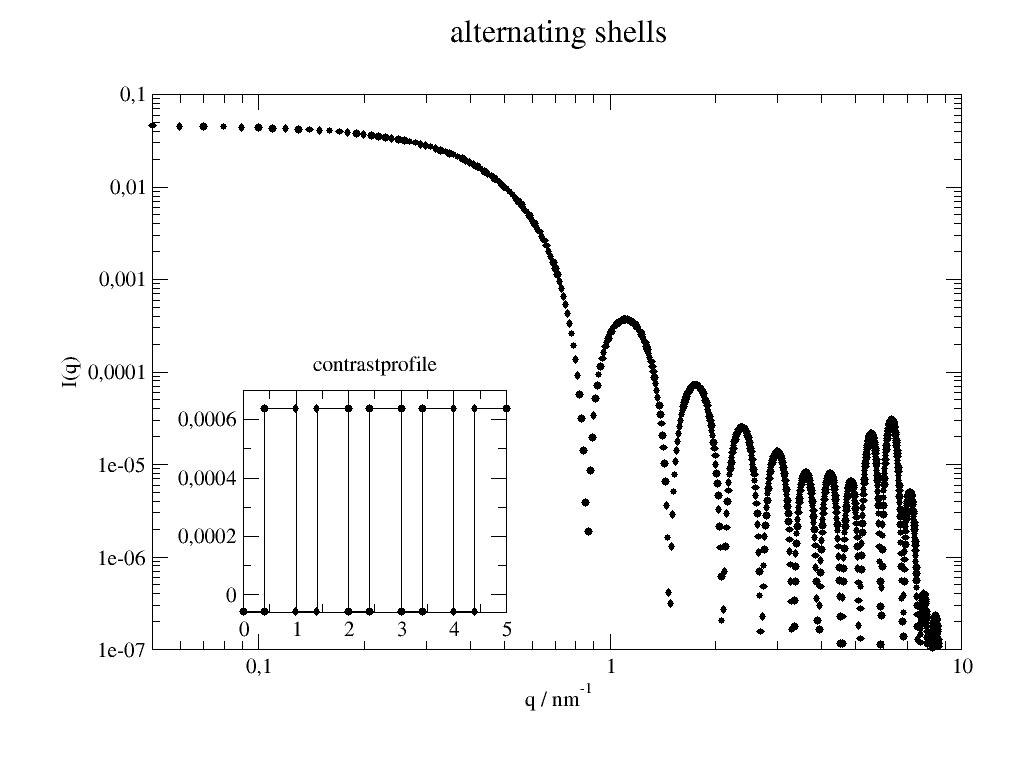
Double shell with exponential decreasing exterior shell to solvent scattering:
import jscatter as js
import numpy as np
x=np.r_[0.0:5:0.01]
def doubleexpshells(q,d1,d2,e3,sd1,sd2,sol,bgr):
   fq = js.ff.multiShellSphere(q,[d1,d2,e3*3],[sd1,sd2,((sd2-sol)*np.exp(-np.r_[0:3:9j]))+sol],solventSLD=sol)
   fq.Y = fq.Y + bgr
   return fq

dde=doubleexpshells(x,0.5,0.5,1,1e-4,2e-4,0,1e-10)
dde1=doubleexpshells(x,0.5,0.1,0.5,1e-4,3e-4,0,1e-10)

#plot it
p=js.grace(1,1)
p.multi(2,1)
p[0].plot(dde,le='thick shell')
p[0].plot(dde1,le='thin shell')
p[0].yaxis(label='I(q)',min=1e-10,max=3e-4,scale='l')
p[1].xaxis(label='q / nm\S-1')
p[1].plot(dde.contrastprofile,li=1,le='thick shell') # a contour of the SLDs
p[1].plot(dde1.contrastprofile,li=1,le='thin shell')
p[1].yaxis(label='contrast',min=0,max=3e-4)
p[1].xaxis(label='r / nm',min=0,max=5)
p[0].title('core-shell-exp particle')
p[1].legend(x=3,y=0.0002)
#p.save(js.examples.imagepath+'/coreShellExp.jpg')
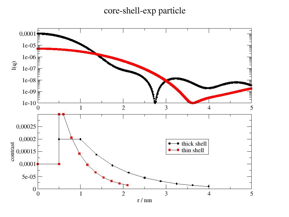
- jscatter.ff.multilamellarVesicles(Q, R, N, phi, displace=0, dR=0, dN=0, nGauss=100, **kwargs)[source]
Scattering intensity of a multilamellar vesicle with random displacements of the inner vesicles [1].
The result contains the full scattering, the structure factor of the lamella and a multilayer formfactor of the lamella layer structure. Other layer structures as mentioned in [2]. Multilayer formfactor is described in
multilayer().- Parameters:
- Qfloat
Wavevector in 1/nm.
- Rfloat
Outer radius of the Vesicle in units nm.
- dRfloat
Width of outer radius distribution in units nm.
- displacefloat
Displacements of the vesicle centers in units nm. This describes the displacement steps in a random walk of the centers. displace=0 it is concentric, all have same center. displace< R/N.
- Nint
Number of lamella.
- dNint, default=0
Width of distribution for number of lamella. (dN< 0.4 is single N) A zero truncated normal distribution is used with N>0 and N<R/displace. Check .Ndistribution and .Nweight = Nweight for the resulting distribution.
- phifloat
Volume fraction \(\phi\) of layers inside of vesicle.
- nGaussint, default 100
Number of Gaussian quadrature points in integration over dR distribution.
- Lamella formfactor parameters (see multilayer)
- layerdlist of float
Thickness of box layers in units nm. List gives consecutive layer thickness from center to outside.
- layerSLDlist of float
Scattering length density of box layers in units 1/nm². Total scattering per box layer is layerSLD[i]*layerd[i]
- gaussposlist of float
Centers of gaussians layers in units nm.
- gausswlist of float
Width of Gaussian.
- gaussSLDlist of float
Scattering length density of Gaussians layers in 1/nm². Total scattering per Gaussian layer is gaussSLD[i]*gaussw[i]
- dsfloat
Gaussian thickness fluctuation (sigma=ds) of central layer in above lamella in nm. The thickness of the central layer is varied and all consecutive position are shifted (gausspos + layer edges).
- solventSLDfloat, default=0
Solvent scattering length density in 1/nm².
- Returns:
- dataArray
- Columns [q,I(q),S(q),F(q)]
I(q)=S(q)F(q) scattering intensity
S(q) multilamellar vesicle structure factor
F(q) lamella formfactor
.columnname=’q;Iq;Sq;Fq’
.outerShellVolume
.Ndistribution
.Nweight
.displace
.phi
.layerthickness
.SLD
.solventSLD
.shellfluctuations=ds
.preFactor=phi*Voutershell**2
- Multilayer attributes (see multilayer)
.contrastprofile ….
Notes
The left shows a concentric lamellar structure. The right shows the random path of the consecutive centers of the spheres. See Multilamellar Vesicles for resulting scattering curves.
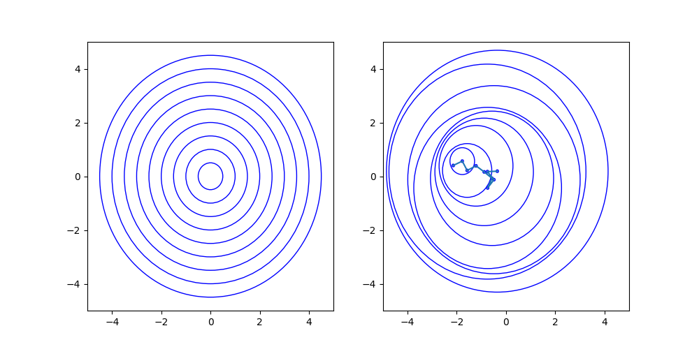
The function returns I(Q) as (see [1] equ. 17 )
\[I(Q)=\phi V_{outershell} S(Q) F(Q)\]with the multishell structure factor \(S(Q)\) as described in [1]. For a single layer we have the formfactor F(Q)
\[F(Q)= ( \sum_i \rho_i d_i sinc( Q d_i) )^2\]with \(\rho_i\) as scattering length density and thickness \(d_i\). For a complex multilayer we find (see
multilayer())\[F(Q)= \sum_{i,j} \rho_i\rho_j d_i d_j sinc(qd_i)sinc(qd_j)cos(q(a_i-a_j))\]with \(a_i\) as positions of the layers.
The amphiphile concentration phi is roughly given by phi = d/a, with d being the bilayer thickness and a being the spacing of the shells. The spacing of the shells is given by the scattering vector of the first correlation peak, i.e., a = 2pi/Q. Once the MLVs leave considerable space between each other then phi < d/a holds. This condition coincides with the assumption of dilution of the Guinier law. (from [1])
Structure factor part is normalized that \(S(0)=\sum_{j=1}^N (j/N)^2\)
To use a different shell form factor the structure factor is given explicitly.
Comparing a unilamellar vesicle (N=1) with multiShellSphere shows that R is located in the center of the shell:
import jscatter as js
import numpy as np
Q=js.loglist(0.0001,5,1000)#np.r_[0.01:5:0.01]
ffmV=js.ff.multilamellarVesicles
p=js.grace()
p.multi(1,2)
# comparison single layer
mV=ffmV(Q=Q, R=100., displace=0, dR=0,N=1,dN=0, phi=1,layerd=6, layerSLD=1e-4)
p[0].plot(mV)
p[0].plot(js.ff.multiShellSphere(Q,[97,6],[0,1e-4]),li=[1,1,3],sy=0)
# triple layer
mV1=ffmV(Q=Q, R=100., displace=0, dR=0,N=1,dN=0, phi=1,layerd=[1,4,1], layerSLD=[0.07e-3,0.6e-3,0.07e-3])
p[1].plot(mV1,sy=[1,0.5,2])
p[1].plot(js.ff.multiShellSphere(Q,[97,1,4,1],[0,0.07e-3,0.6e-3,0.07e-3]),li=[1,1,4],sy=0)
p[1].yaxis(label='S(Q)',scale='l',min=1e-10,max=1e6,ticklabel=['power',0])
p[0].yaxis(label='S(Q)',scale='l',min=1e-10,max=1e6,ticklabel=['power',0])
p[1].xaxis(label='Q / nm\S-1',scale='l',min=1e-3,max=5,ticklabel=['power',0])
p[0].xaxis(label='Q / nm\S-1',scale='l',min=1e-3,max=5,ticklabel=['power',0])
References
[1] (1,2,3,4,5)Small-angle scattering model for multilamellar vesicles H. Frielinghaus Physical Review E 76, 051603 (2007)
[2]Small-Angle Scattering from Homogenous and Heterogeneous Lipid Bilayers N. Kučerka Advances in Planar Lipid Bilayers and Liposomes 12, 201-235 (2010)
Examples
- Scattering length densities and sizes roughly for DPPC from
Kučerka et al. Biophysical Journal. 95,2356 (2008) https://doi.org/10.1529/biophysj.108.132662
The SAX scattering is close to matching resulting in low scattering at low Q. The specific structure depends on the lipid composition and layer thickness. Kučerka uses a multi (n>6) Gauss profile where we use here approximate values in a simple 3 layer box profile to show the main characteristics.
import jscatter as js
import numpy as np

ffmV=js.ff.multilamellarVesicles
Q=js.loglist(0.02,8,500)
dd=1.5
dR=5
nG=100
R=50
N=3
ds=0.05
st=[0.75,2.8,0.75]
p=js.grace(1,1)
p.title('Lipid bilayer in SAXS/SANS')

# SAXS
sld=np.r_[420,290,420]*js.formel.felectron  # unit e/nm³*fe
sSLD=335*js.formel.felectron  # H2O unit e/nm³*fe
saxm=ffmV(Q=Q, R=R, displace=dd, dR=dR,N=N,dN=0, phi=0.2,layerd=st, layerSLD=sld,solventSLD=sSLD,nGauss=nG,ds=ds)
p.plot(saxm,sy=[1,0.3,1],le='SAXS multilamellar')
saxu=ffmV(Q=Q, R=R, displace=0, dR=dR,N=1,dN=0, phi=0.2,layerd=st, layerSLD=sld,solventSLD=sSLD,nGauss=100,ds=ds)
p.plot(saxu,sy=0,li=[1,2,4],le='SAXS unilamellar')

# SANS
sld=[4e-4,-.5e-4,4e-4]  # unit 1/nm²
sSLD = 6.335e-4 # D2O
sanm=ffmV(Q=Q, R=R, displace=dd, dR=dR,N=N,dN=0, phi=0.2,layerd=st, layerSLD=sld,solventSLD=sSLD,nGauss=nG,ds=ds)
p.plot( sanm,sy=[1,0.3,2],le='SANS multilamellar')
sanu=ffmV(Q=Q, R=R, displace=0, dR=dR,N=1,dN=0, phi=0.2,layerd=st, layerSLD=sld,solventSLD=sSLD,nGauss=100,ds=ds)
p.plot(sanu,sy=0,li=[1,2,3],le='SANS unilamellar')
#
p.legend(x=1.3,y=1)
p.subtitle(f'R=50 nm, N={N}, layerthickness={st} nm, dR=5')
p.yaxis(label='S(Q)',scale='l',min=1e-6,max=1e4,ticklabel=['power',0])
p.xaxis(label='Q / nm\S-1',scale='l',min=2e-2,max=20,ticklabel=['power',0])

# contrastprofile
p.new_graph( xmin=0.6,xmax=0.95,ymin=0.7,ymax=0.88)
p[1].plot(saxu.contrastprofile,li=[1,4,1],sy=0)
p[1].plot(sanu.contrastprofile,li=[1,4,2],sy=0)
p[1].xaxis(label='multiayerprofile')
p[1].yaxis(label='contrast')
#p.save(js.examples.imagepath+'/multilamellarVesicles.jpg')
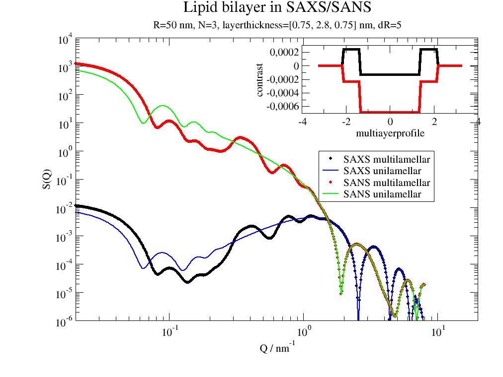
- jscatter.ff.multilayer(q, layerd=None, layerSLD=None, gausspos=None, gaussw=None, gaussSLD=None, ds=0, solventSLD=0)[source]
Form factor of a multilayer with rectangular/Gaussian density profiles perpendicular to the layer.
To describe smeared interfaces or complex profiles use more layers.
- Parameters:
- qarray
Wavevectors in units 1/nm.
- layerdlist of float
Thickness of box layers in units nm. List gives consecutive layer thickness from center to outside.
- layerSLDlist of float
Scattering length density of box layers in units 1/nm². Total scattering per box layer is (layerSLD[i]*layerd[i])²
- gaussposlist of float
Centers of gaussians layers in units nm.
- gausswlist of float
Width of Gaussian.
- gaussSLDlist of float
Scattering length density of Gaussians layers in 1/nm². Total scattering per Gaussian layer is (gaussSLD[i]*gaussw[i])²
- dsfloat, list
- float
Gaussian thickness fluctuation (sigma=ds) of central layer in above lamella in nm. The thickness of the central layer is varied and all consecutive position are shifted (gausspos + layer edges).
- list, ds[0]=’outersld’,’innersld’,’inoutsld’,’centersld’, ds[1..n+1]= w[i]
SLD fluctuations in a layer. The factor 0 < f[i]=i/n < 1 determines the SLD of the outer layer occurring with a probability w[i] as f[i]*sld. E.g. parabolic profile
ds=['outersld',np.r_[0:1:7j]**2]or upper halfds=['outersld',np.r_[0,0,0,0,1,1,1,1]]
- solventSLDfloat, default=0
Solvent scattering length density in 1/nm².
- Returns:
- dataArray
- Columns [q, Fq, Fa2]
Fq \(F(q)=<\sum_{ij} F_a(q,i)F_a^*(q,j)>\) is multilayer scattering per layer area.
Fa2 \(Fa2(q)=<\sum_{i} F_a(q,i)>^2\) described fluctuations in the multilayer for given ds. Might be used for stacks of multilayers and similar.
To get the scattering intensity of a volume the result needs to be multiplied with the layer area [2].
.contrastprofile contrastprofile as contrast to solvent SLD.
.profilewidth
Notes
The scattering amplitude \(F_a\) is the Fourier transform of the density profile \(\rho(r)\)
\[F_a(q)=\int \rho(r)e^{iqr}dr\]For a rectangular profile [1] of thickness \(d_i\) centered at \(a_i\) and layer scattering length density \(\rho_i\) we find
\[F_{a,box}(q)= \rho_i d_i sinc(qd_i/2)e^{iqa_i}\]For a Gaussian profile [2] \(\rho(r) = \frac{\rho_i}{\sqrt{2\pi}}e^{-r^2/s_i^2/2}\) with width \(s_i\) and same area as the rectangular profile \(\rho_is_i = \rho_id_i\) we find
\[F_{a,gauss}(q)= \rho_i s_i e^{-(q^2s_i^2/2)}e^{iqa_i}\]The scattering amplitude for a multi box/gauss profile is \(F_a(q)=\sum_i F_a(q,i)\)
The formfactor \(F(q)\) of this multi layer profile is in average \(<>\)
\[F(q)=<\sum_{ij} F_a(q,i)F_a^*(q,j)>\]resulting e.g. for a profile of rectangular boxes in
\[F_{box}(q)=\sum_{i,j} \rho_i\rho_j d_i d_j sinc(qd_i)sinc(qd_j)cos(q(a_i-a_j))\]- To get the 3D orientational average one has 2 options:
add a Lorentz correction \(q^{-2}\) to describe the correct scattering in isotropic average (see [2]). Contributions of multilamellarity resulting in peaky structure at low Q are ignored.
Use multilamellarVesicles which includes a full structure factor and also size averaging. The Lorentz correction is included as the limiting case for high Q. Additional the peaky structure at low Q is described as a consequence of the multilamellarity. See Multilamellar Vesicles for examples.
Approximately same minimum for gaussian and box profiles is found for \(s_i = d_i/\pi\). To get same scattering I(0) the density needs to be scaled \(\rho_i\pi\).
- Restricting parameters for Fitting
If the model is used during fits one has to consider dependencies between the parameters to restrict the number of free parameters. Symmetry in the layers may be used to restrict the parameter space.
References
[1]Modelling X-ray or neutron scattering spectra of lyotropic lamellar phases : interplay between form and structure factors F. Nallet, R. Laversanne, D. Roux Journal de Physique II, EDP Sciences, 1993, 3 (4), pp.487-502 https://hal.archives-ouvertes.fr/jpa-00247849/document
[2] (1,2)X-ray scattering from unilamellar lipid vesicles Brzustowicz and Brunger, J. Appl. Cryst. (2005). 38, 126–131
[3]Structural information from multilamellar liposomes at full hydration: Full q-range fitting with high quality X-ray data. Pabst, G., Rappolt, M., Amenitsch, H. & Laggner, P. Phys. Rev. E - Stat. Physics, Plasmas, Fluids, Relat. Interdiscip. Top. 62, 4000–4009 (2000).
Examples
Some symmetric box and gaussian profiles in comparison. An exact match is not possible but the differences are visible only in higher order lobes.
import jscatter as js
import numpy as np
q=np.r_[0.01:5:0.001]
p=js.grace()
p.multi(2,1)
p[0].title('multilayer membranes')
p[0].text(r'I(0) = (\xS\f{}\si\NSLD[i]*width[i])\S2',x=0.5,y=80)
p[0].text(r'equal minimum using \n2width\sgauss\N=width\sbox\N 2/\xp', x=0.7, y=25)
profile=np.r_[2,1,2]
#
pf1=js.ff.multilayer(q,layerd=[1,5,1],layerSLD=profile)
p[0].plot(pf1,sy=[1,0.3,1],le='box')
p[1].plot(pf1.contrastprofile,li=[1,2,1],sy=0,le='box only')
#
# factor between sigma and box width
f=2 * 3.141/2
pf2=js.ff.multilayer(q,gausspos=np.r_[0.5,3.5,6.5],gaussSLD=profile*f,gaussw=np.r_[1,5,1]/f)
p[0].plot(pf2,sy=[2,0.3,2],le='gauss')
p[1].plot(pf2.contrastprofile,li=[1,2,2],sy=0,le='gauss only')
#
pf3=js.ff.multilayer(q,layerd=[1,5,1],layerSLD=[0,1,0],gausspos=np.r_[0.5,6.5],gaussSLD=[2*f,2*f],gaussw=np.r_[1,1]/f)
p[0].plot(pf3,sy=[3,0.3,3],le='gauss-box-gauss')
p[1].plot(pf3.contrastprofile,li=[1,2,3],sy=0,le='gauss-box-gauss')

pf3=js.ff.multilayer(q,layerd=[1,5,1],layerSLD=[0,1,0],gausspos=np.r_[0.5,6.5],gaussSLD=[2*f,2*f],gaussw=np.r_[1,1]/f,ds=0.8)
p[0].plot(pf3,sy=0,li=[1,2,4],le='gauss-box-gauss with fluctuations')
p[1].plot(pf3.contrastprofile,li=[1,2,4],sy=0,le='gauss-box-gauss')

p[0].yaxis(scale='n',min=0.001,max=90,label='I(Q)',charsize=1)#,ticklabel=['power',0,1]
p[0].xaxis(label='',charsize=1)
p[1].yaxis(label='contrast profile ()')
p[0].xaxis(label='position / nm')
p[1].xaxis(label='Q / nm\S-1')
p[0].legend(x=2.5,y=70)
#p.save(js.examples.imagepath+'/multilayer.jpg')
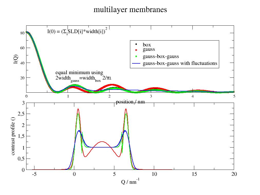
How to use in a fit model Due to the large number of possible models (e.g. 9 Gaussians with each 3 parameters), smearing and more one has to define what seems to be important and use symmetries to reduce the parameter space.
Complex profiles with tens of layers are possible and may be defined like this:
# 5 layer box model
def box5(q,d1,d2,d3,s1,s2):
   # symmetric model with 5 layers, d1 central, d3 outer
   # outer layers have half the scattering length density of d2
   result=js.ff.multilayer(q,layerd=[d3,d2,d1,d2,d3],layerSLD=[s2/2,s2,s1,s2,s2/2],solventSLD=0)
   return result
A model of Gaussians We describe a symmetric bilayer with a center Gaussian and 2 Gaussians at each side to describe the head groups.
# define symmetric 3 gaussian model according to positions p_i of the Gaussian centers.
def gauss3(q,p1,p2,s1,s2,s0,w1,w2,w0):
    # define your model
    p0=0
    pos = np.r_[-p2,-p1,p0,p1,p2]  # symmetric positions
    result=js.ff.multilayer(q,gausspos=pos,gaussSLD=[s2,s1,s0,s1,s2],gaussw=[w2,w1,w0,w1,w2],solventSLD=0)
    return result
- jscatter.ff.orientedCloudScattering(qxzw, cloud, mosaicity=None, formfactoramp=None, rms=0, V=None, nCone=50, ncpu=0)[source]
Oriented 3D scattering of a cloud of isotropic particles.
Cloud can represent an object/lattice described by a cloud of isotropic scatterers to describe formfactors or structure factors.
Scattering amplitudes may be constant, sphere scattering amplitude, Gaussian scattering amplitude or explicitly given form factor.
For mean cloud particle distance d one expects Bragg peaks or structure factor peaks around 2π/d.
In a scattering geometry with the incoming beam along the cloud z-axis a flat small angle detector depicts the projection of the Ewald sphere onto the \(q_xq_y\)-plane (see sas). Only for small angle scattering one might assume z=0.
Instead of rotating the cloud by rotation matrix \(R\) we may rotate the reciprocal space by \(R^T\) to result in a rotating crystal method.
- Parameters:
- qxzwarray, ndim= Nx3
3D wavevectors in 1/nm. Wavevectors may represent a line, a plane or any other 3D distribution in reciprocal space (e.g. Ewald-sphere surface). If 2D (ndim=Nx2) the 3rd dim is set to zero.
- cloudarray Nx3, Nx4, Nx5
Positions (center of mass) and type of particles.
cloud[:,3] Center of mass positions (in nm) of the N scatterers in the cloud.
cloud[:,3] scattering length \(b\) at positions cloud[:,:3], optional, otherwise \(b=1\).
cloud[:,4] column index in formfactoramp for a specific scatterer, optional.
- rmsfloat, default=0
Root mean square displacement :math:`langleu^2rangle^{0.5} of the positions in cloud as random displacements in nm. The displacement is randomly chosen for each orientation (nCone). rms can be used to simulate a Debye-Waller factor. nCone>>50 with mosaicity>0 or rms>0 is advised to yield reasonable average and reduced noise .
- mosaicitylist 3 float, default None
Mosaicity describes a Gaussian distribution of crystallite orientations around a reference orientation [1]. The mosaicity is commonly equated with the standard deviation of the Gaussian [2]. Here mosaicity = [width, phi, theta] (units rad) with
width - >0 : Gaussian distribution weight (cut at π) with width=sigma. - <0 : equal weight within width.
phi as azimuthal angle of reference orientation in spherical coordinates (phi=0, theta=π/2 is x axis)
theta as altitude angle of reference orientation in spherical coordinates (theta=0 is Z axis)
3° around the X-axis [np.deg2rad(3),0,π/2]
5° around the Y-axis [np.deg2rad(5),π/2,π/2]
5° around the Z-axis [np.deg2rad(5),0,0]
Integration is limited to 2.5*sigma in the Gaussian.
- nConeint
Number of points in mosaicity distribution as Fibonacci lattice points.
- formfactorampNone,’gauss’,’sphere’,’cube’
Normalized scattering amplitudes of cloud points \(\hat{F_a^i}(q)\). \(F_a(q)=b_i \hat{F_a^i}(q)\) with bi from cloud[3].
None : const scattering amplitude.
- ‘sphere’: Sphere scattering amplitude according to [3] equal for all cloud points.
Parameter V is needed to determine \(R\). The sphere radius is \(R=(\frac{3V}{4\pi})^{1/3}\)
- ‘gauss’Gaussian function \(\hat{F_a}(q) = exp(-\pi V^{2/3}q^2)\) according to [2]
Equal for all cloud points. The Gaussian shows no artificial minima compared to the sphere. Use parameter V to determine \(b_i\).
- ‘coil’Polymer coil (ideal Gaussian chain) showing scattering according to Debye function equal for all.
Parameter V needed to determine \(R_g = (\frac{3V}{4\pi})^{1/3}\). The scattering length is \(b_i = Nb_{monomer}\) with monomer number \(N\).
- Explicit isotropic \(\hat{F_a}(q)\) as array with [q,fa1(q),fa2(q),fa3(q),….].
If multiple fai are given the index i for a cloud point needs to be given in cloud[4]
The normalized scattering amplitude fa for each cloud point is calculated as fa=fai/fai[0]. Missing values are linear interpolated, q values outside interval are mapped to qmin or qmax.
Explicit formfactoramps are assumed to be isotropic.
If the scattering amplitude is not known \(F_a(q) \approx F^{1/2}(q)\) might be used as approximation for low Q.
- Vfloat, default=None
Volume of the scatterers to determine scattering amplitude (see formfactoramp). Only needed for formfactoramp ‘sphere’ and ‘gauss’.
- ncpuint, default 0
- Number of cpus used in the pool for multiprocessing.
not given or 0 : all cpus are used
int>0 : min(ncpu, mp.cpu_count)
int<0 : ncpu not to use
1 : single core usage for testing or comparing speed to Debye
- Returns:
- dataArray
- Columns [qx, qz, qw, Pq]
The forward scattering is Pq(q=0)= sumblength**2
.sumblength : Sum of blength with sumblength**2
.formfactoramplitude : formfactoramplitude of cloudpoints according to type for all q values.
.formfactoramplitude_q :corresponding q values.
References
[1]Kotlarchyk and S.-H. Chen, J. Chem. Phys. 79, 2461 (1983).1
[2] (1,2)An improved method for calculating the contribution of solvent to the X-ray diffraction pattern of biological molecules Fraser R MacRae T Suzuki E IUCr Journal of Applied Crystallography 1978 vol: 11 (6) pp: 693-694
[3]X-ray diffuse scattering by proteins in solution. Consideration of solvent influence B. A. Fedorov, O. B. Ptitsyn and L. A. Voronin J. Appl. Cryst. (1974). 7, 181-186 doi: 10.1107/S0021889874009137
Examples
How to use orientedCloudScattering for fitting see last Example in cloudScattering.
Two point particles on y-axis result in pattern cos**2, Mosaicity creates incomplete 2d Debye-Scherer like rings. rms smears larger q.
import jscatter as js
import numpy as np
from scipy.spatial.transform import Rotation

# detector planes for z=0, y=0, x=0
q = np.mgrid[-6:6:51j, -6:6:51j].reshape(2,-1).T
qz =np.c_[q,np.zeros_like(q[:,0])]  # flat detector in experiment has z!=0
qy = (Rotation.from_euler('x',np.pi/2).as_matrix() @ qz.T).T
qx = (Rotation.from_euler('y',np.pi/2).as_matrix() @ qz.T).T

# to show as cube surfaces
fig = js.mpl.figure(figsize=[8, 3],dpi=200)
ax1 = fig.add_subplot(1, 4, 1, projection='3d')
ax2 = fig.add_subplot(1, 4, 2, projection='3d')
ax3 = fig.add_subplot(1, 4, 3, projection='3d')
ax4 = fig.add_subplot(1, 4, 4, projection='3d')
fig.suptitle('Two points along Y')

# two points (constant formfactor)
rod2=np.zeros([2,3])
rod2[:,1]=np.r_[0,np.pi]  # position on y axis

mo = [np.deg2rad(5),0,0]
ffz2 = js.ff.orientedCloudScattering(qz,rod2,rms=0,mosaicity=mo,nCone=50)
ffy2 = js.ff.orientedCloudScattering(qy,rod2,rms=0,mosaicity=mo,nCone=50)
ffx2 = js.ff.orientedCloudScattering(qx,rod2,rms=0,mosaicity=mo,nCone=50)
ax = js.mpl.contourOnCube(ffz2[[0,1,3]].array,ffx2[[1,2,3]].array,ffy2[[0,2,3]].array,offset=[-6,-6,6], ax=ax1)
ax.set_title('5° mosaicity \nalong z-axis',size='small')

mo = [np.deg2rad(25),0,0]
ffz2 = js.ff.orientedCloudScattering(qz,rod2,rms=0,mosaicity=mo,nCone=150)
ffy2 = js.ff.orientedCloudScattering(qy,rod2,rms=0,mosaicity=mo,nCone=150)
ffx2 = js.ff.orientedCloudScattering(qx,rod2,rms=0,mosaicity=mo,nCone=150)
ax = js.mpl.contourOnCube(ffz2[[0,1,3]].array,ffx2[[1,2,3]].array,ffy2[[0,2,3]].array,offset=[-6,-6,6], ax=ax2)
ax.set_title('25° mosaicity \n along z-axis',size='small')

mo = np.deg2rad([45,0,90])
ffz2 = js.ff.orientedCloudScattering(qz,rod2,rms=0,mosaicity=mo,nCone=150)
ffy2 = js.ff.orientedCloudScattering(qy,rod2,rms=0,mosaicity=mo,nCone=150)
ffx2 = js.ff.orientedCloudScattering(qx,rod2,rms=0,mosaicity=mo,nCone=150)
ax = js.mpl.contourOnCube(ffz2[[0,1,3]].array,ffx2[[1,2,3]].array,ffy2[[0,2,3]].array,offset=[-6,-6,6], ax=ax3)
ax.set_title('45° mosaicity \n along x-axis',size='small')

mo = [np.deg2rad(25),0,0]
ffz2 = js.ff.orientedCloudScattering(qz,rod2,rms=0.2,mosaicity=mo,nCone=150)
ffy2 = js.ff.orientedCloudScattering(qy,rod2,rms=0.2,mosaicity=mo,nCone=150)
ffx2 = js.ff.orientedCloudScattering(qx,rod2,rms=0.2,mosaicity=mo,nCone=150)
ax = js.mpl.contourOnCube(ffz2[[0,1,3]].array,ffx2[[1,2,3]].array,ffy2[[0,2,3]].array,offset=[-6,-6,6], ax=ax4)
ax.set_title('25°mosaicity +rms=0.2 \n along x-axis',size='small')

#ax.figure.savefig(js.examples.imagepath+'/cloudMosaicity.jpg')
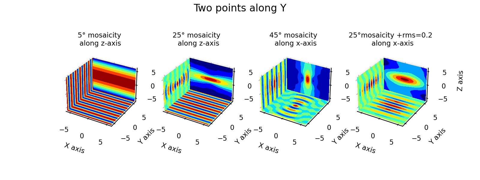
Same as above for a cubic grid of 5x5x5 point particles using
cube = js.lattice.scLattice(2,[2,2,2]).XYZ
See example example_orientedCloudCube.py
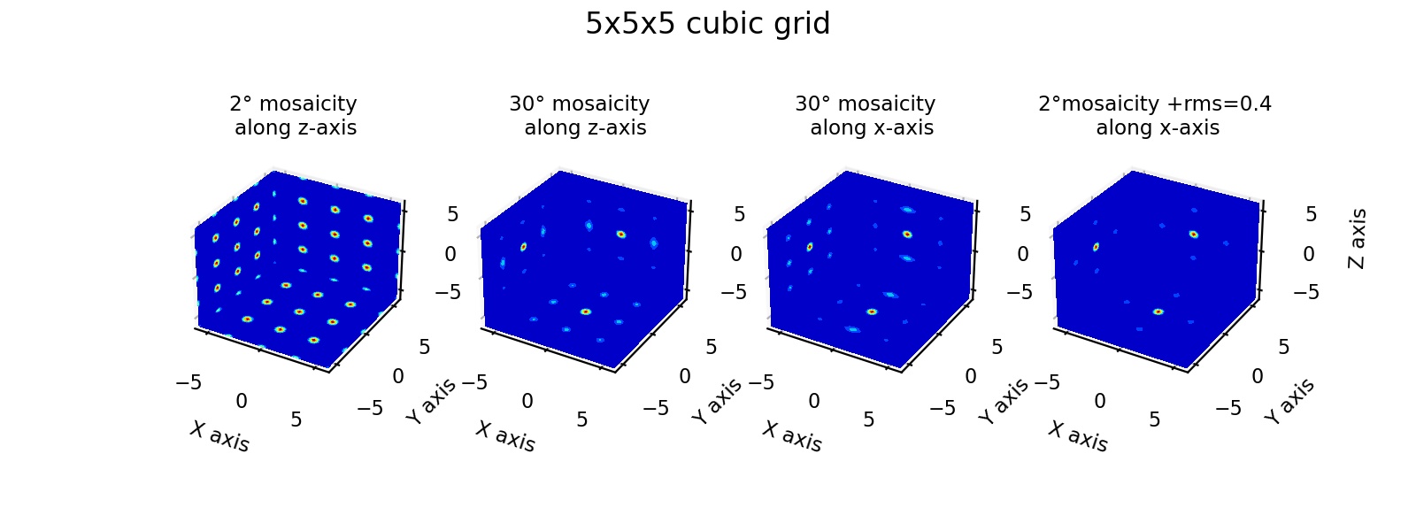
5 spheres in line with small position distortion and mosaicity 20° around z-axis:
import jscatter as js
import numpy as np
rod0 = np.zeros([5, 3])
rod0[:, 1] = np.r_[0, 1, 2, 3, 4] * 3
qxzw = np.mgrid[-6:6:50j, -6:6:50j].reshape(2, -1).T
mo = [np.deg2rad(20),0,0]
ffe = js.ff.orientedCloudScattering(qxzw,rod0,formfactoramp='sphere',V=4/3.*np.pi*2**3,mosaicity=mo,rms=0.02)
fig4 = js.mpl.surface(ffe.X, ffe.Z, np.log10(ffe.Y), colorMap='gnuplot')
fig4.axes[0].set_title('5 spheres with R=2 along Z with noise (rms=0.02)')
fig4.show()
Solution of oriented particle-composite of 3 touching core shell particles with small position distortion. Here we add a isotropic Percus-Yevick structure factor as effective composite interaction between particle composites.
The particles are oriented along x-axis to a tumbling around x-axis is represented by x-axis mosaicity
import jscatter as js
import numpy as np
N=6    # number of particles
Rc=2   # core radius
Rs=6   # outer shell radius
d=Rs*2 # distance of particles
volumefraction=0.10  # single particles
rms=1.5
# position composite particles along X axis
rod0 = np.zeros([N, 3])
rod0[:, 0] = np.r_[0:N] * d  # positions
# q grid
qxzw = np.mgrid[-2:2:150j, -2:2:150j].reshape(2, -1).T
# core shell formfactoramp for particles and use interpolation
q = js.loglist(0.01, 7, 100)
cs = js.ff.sphereCoreShell(q=q, Rc=Rc, Rs=Rs, bc=-0.1, bs=1, solventSLD=0)
csa = cs[[0,2]]
# oriented composite scattering
ffe = js.ff.orientedCloudScattering(qxzw, rod0, formfactoramp=csa, mosaicity=np.deg2rad([5,0,90]), rms=rms)
fig4a = js.mpl.contourImage(ffe.X, ffe.Z, ffe.Y, colorMap='gnuplot',scale='log')
fig4a.axes[0].set_title('3 core shell particles with R=2 along X with noise')

# add structure factor according to radial q component
sf=js.sf.PercusYevick(q, Rs*N/2, eta=volumefraction*N)  # approximate higher radius
qradial=np.linalg.norm(ffe[:3],axis=0)
ffe.Y=ffe.Y*sf.interp(qradial)
fig4b = js.mpl.contourImage(ffe.X, ffe.Z, ffe.Y, colorMap='gnuplot',scale='log')
fig4b.axes[0].set_title('3 core shell particles with noise and interparticle interaction ')
#fig4b.savefig(js.examples.imagepath+'/orientedCloudScattering.jpg')
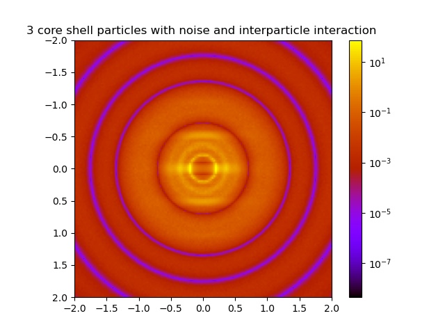
Make a slice for an angular region but with higher resolution to see the additional peaks due to alignment
import jscatter as js
import numpy as np
# rod0 will be position of 5 points in a row
rod0 = np.zeros([5, 3])
rod0[:, 1] = np.r_[0, 1, 2, 3, 4] * 3

qxzw = np.mgrid[-4:4:150j, -4:4:150j].reshape(2, -1).T    # xz plane grid
# only as demo : extract q from qxzw
qxzw = np.c_[qxzw, np.zeros_like(qxzw[:, 0])]              # add y=0 component
qrpt = js.formel.xyz2rphitheta(qxzw)                     # spherical coordinates
q = np.unique(sorted(qrpt[:, 0]))

# or use interpolation; cs will be our formfactoramp
q = js.loglist(0.01, 7, 100)
cs = js.ff.sphereCoreShell(q=q, Rc=1, Rs=2, bc=0.1, bs=1, solventSLD=0)
csa = cs[[0,2]]

# calc scattering in plane qxzw
ffe = js.ff.orientedCloudScattering(qxzw, rod0, formfactoramp=csa, mosaicity=np.deg2rad([5,0,0]), nCone=100, rms=0.05)

# show it in surface plot
fig4 = js.mpl.surface(ffe.X, ffe.Z, np.log10(ffe.Y), colorMap='gnuplot')
fig4.axes[0].set_title('5 core shell particles with R=2 along Z with noise (rms=0.05)')
fig4.show()

# We do an explicit radial average
# transform X,Z to spherical coordinates
qphi=js.formel.xyz2rphitheta([ffe.X,ffe.Z,np.zeros_like(ffe.X)],transpose=True )[:,:2]
# add qphi or use later rp[1] for selection
ffb=ffe.addColumn(2,qphi.T)
# select a portion of the phi angles
phi=np.pi/2
dphi=0.2
ffn=ffb[:,(ffb[-1]<phi+dphi)&(ffb[-1]>phi-dphi)]
ffn.isort(-2)    # sort along radial q
p=js.grace()
p.plot(ffn[-2],ffn.Y,le='oriented spheres form factor')
# compare to coreshell formfactoramp scaled
p.plot(cs.X,csa.Y**2/cs.Y[0]*25,li=1,le='coreshell form factor')
p.yaxis(label='F(Q,phi=90°+-11°)', scale='log')
p.title('5 aligned core shell particle with additional interferences',size=1.)
p.subtitle(' due to sphere alignment dependent on observation angle')

# 2: direct way with 2D q in xz plane
rod0 = np.zeros([5, 3])
rod0[:, 1] = np.r_[0, 1, 2, 3, 4] * 3
x=np.r_[0.0:6:0.05]
qxzw = np.c_[x, x*0,x*0]
for alpha in np.r_[0:91:30]:
    R=js.formel.rotationMatrix(np.r_[0,0,1],np.deg2rad(alpha)) # rotate around Z axis
    qa=np.dot(R,qxzw.T).T[:,:2]
    mo=np.deg2rad([5,0,0])
    ffe = js.ff.orientedCloudScattering(qa, rod0, formfactoramp=csa, mosaicity=mo, nCone=100, rms=0.05)
    p.plot(x,ffe.Y,li=[1,2,-1],sy=0,le='alpha=%g' %alpha)
p.xaxis(label=r'Q / nm\S-1')
p.legend()
- jscatter.ff.orientedCloudScattering3Dff(qxzw, cloud, mosaicity=None, formfactoramp=None, rms=0, dorient=0, nCone=None, ncpu=0)[source]
Oriented 3D scattering of a cloud of non-isotropic particles.
Cloud can represent an object/lattice described by a cloud of equal non-isotropic scatterers as e.g. as a lattice of oriented cuboids or ellipsoids.
Anisotropic formfactor amplitudes are fa_cuboid, fa_ellipsoid, fa_disc or can be calculated using orientedCloudScattering(…)[[0,1,2,4]] e.g. for sphere twins, triples or any other shape.
For mean cloud particle distance d one expects Bragg peaks or structure factor peaks around 2π/d.
In a scattering geometry with the incoming beam along the cloud z-axis a flat small angle detector depicts the projection of the Ewald sphere onto the \(q_xq_y\)-plane (see sas). Only for small angle scattering one might assume z=0.
Instead of rotating the cloud by rotation matrix \(R\) we may rotate the reciprocal space by \(R^T\) to result in a rotating crystal method.
- Parameters:
- qxzwarray, ndim= Nx3, Nx2
3D wavevectors (unit 1/nm) may represent a plane (e.g. detector plane) or any other 3D distribution in reciprocal space as a line or the surface of the Ewald sphere.
If 2D the 3rd dim (w) is set to zero for convenience.
- cloudarray Nx3, Nx4, Nx5, Nx6, Nx7
Positions (center of mass) and orientations of individual particles in the cloud. Orientation angles describe the rotation of the non-isotropic scatterer relative to the used 3D formfactoramp with yaw, pitch and roll angle as rotations around (in order) z-y’-x” (intrinsic) or x-y-z axes (extrinsic) leading to \(R = R_z(\theta) R_y(\phi) R_x(\psi)\).
cloud[:,:3] center of mass positions
cloud[:,3] scattering length \(b_i\)
cloud[:,4] roll angle Ψ [0..2π] around extrinsic x axis.
cloud[:,5] pitch angle φ [0..2π] around extrinsic y axis.
cloud[:,6] yaw angle θ [0..π] around extrinsic z axis.
- mosaicitylist 3 float, default None
Mosaicity describes a Gaussian distribution of crystallite orientations around a reference orientation [1]. The mosaicity is commonly equated with the standard deviation of the Gaussian [2]. Here mosaicity = [width, phi, theta] (units rad) with
- width
>0 : Gaussian distribution weight (cut at π) with width=sigma.
<0 : equal weight within width.
phi as azimuthal angle of reference orientation in spherical coordinates (phi=0, theta=π/2 is x axis)
theta as altitude angle of reference orientation in spherical coordinates (theta=0 is Z axis)
3° around the X-axis [np.deg2rad(3),0,π/2]
5° around the Y-axis [np.deg2rad(5),π/2,π/2]
5° around the Z-axis [np.deg2rad(5),0,0]
Integration is limited to 2.5*sigma in the Gaussian.
- rmsfloat, default=0
Root mean square displacement :math:`langleu^2rangle^{0.5} of the positions in cloud as random displacements in nm. The displacement is randomly chosen for each orientation (nCone). rms can be used to simulate a Debye-Waller factor. nCone>>50 with mosaicity>0 or rms>0 is advised to yield reasonable average and reduced noise.
- dorientfloat, default=0
Width of Gaussian distribution (units rad) of roll,pitch and yaw angles in cloud particle orientation. nCone>>50 with mosaicity>0, rms>0 or dorient>0 is advised to yield reasonable average and reduced noise.
- nConeint, None, default 50
Number of points in mosaicity distribution as Fibonacci lattice points.
- formfactoramparray 4xN
Explicit isotropic formfactor amplitude as array with [qx,qz,qw, fa(qx,qz,qw,)] and q in units 1/nm.
formfactoramp fa(q) is normalized fa->fa/fa(0,0,0).
Missing values are linear interpolated, q values outside interval are mapped to border values.
if shape is (N,4) automatic transpose is used.
- ncpuint, default 0
- Number of cpus used in the pool for multiprocessing.
not given or 0 : all cpus are used
int>0 : min(ncpu, mp.cpu_count)
int<0 : ncpu not to use
1 : single core usage for testing or comparing speed to Debye
- Returns:
- dataArray
- Columns [qx, qz, qw, Pq]
.sumblength : sum of blength with sum(cloud[:,3])
The forward scattering is \(Sq(q=0)= (\sum b_i)^2 = cloud[:,3].sum()^2\)
References
[1]Darwin CG, Phil. Mag. 43, 800-829 (1922). (DOI: 10.1080/14786442208633940)
Examples
**Cubes along line, simple cubic and distorted ** We depict the respective q=0 plane at the surface of a cube to present all 3 orientations.
import jscatter as js
import numpy as np
from scipy.spatial.transform import Rotation

# detector planes; a real flat detector has z>0
q = np.mgrid[-9:9:51j, -9:9:51j].reshape(2,-1).T
qz =np.c_[q,np.zeros_like(q[:,0])]  # for z=0
qy = (Rotation.from_euler('x',np.pi/2).as_matrix() @ qz.T).T
qx = (Rotation.from_euler('y',np.pi/2).as_matrix() @ qz.T).T

# degree of disorder
dorient=0

# a 3D scattering amplitude of an asymmetric cube
N=20
R=np.linalg.norm(qz,axis=1).max()
grid= js.sf.scLattice(R/N,N).XYZ
fa = js.ff.fa_cuboid(*grid[:,:3].T,0.2,0.4,2)

# create a rod of 2 cubes as demo
rod2=np.zeros([2,6]);
rod2[:,1] = np.r_[0,3]      # set y positions
rod2[:,3] = 1               # set b
rod2[:,4] = 0 #np.pi/2      # set azimuth angle φ
rod2[:,5] = 0               # set altitude angle θ
# look only at one
ffz1 = js.ff.orientedCloudScattering3Dff(qz,cloud=rod2[:1], formfactoramp=fa,dorient=dorient)
ffy1 = js.ff.orientedCloudScattering3Dff(qy,cloud=rod2[:1], formfactoramp=fa,dorient=dorient)
ffx1 = js.ff.orientedCloudScattering3Dff(qx,cloud=rod2[:1], formfactoramp=fa,dorient=dorient)

# a rod of 4 cubes
rod4 = np.repeat([np.r_[0,0,0,1,0,0]],4,axis=0)
rod4[:,0] = np.r_[0:6:4j]  # set distance along x axis
ffz4 = js.ff.orientedCloudScattering3Dff(qz,cloud=rod4, formfactoramp=fa,dorient=dorient)
ffy4 = js.ff.orientedCloudScattering3Dff(qy,cloud=rod4, formfactoramp=fa,dorient=dorient)
ffx4 = js.ff.orientedCloudScattering3Dff(qx,cloud=rod4, formfactoramp=fa,dorient=dorient)

# a small lattice of 3x3x3 cubes
square27 = js.lattice.scLattice(2,[1,1,1]).points
square27 = np.hstack([square27,np.zeros([square27.shape[0],2])])
ffz27 = js.ff.orientedCloudScattering3Dff(qz,cloud=square27, formfactoramp=fa,dorient=dorient)
ffy27 = js.ff.orientedCloudScattering3Dff(qy,cloud=square27, formfactoramp=fa,dorient=dorient)
ffx27 = js.ff.orientedCloudScattering3Dff(qx,cloud=square27, formfactoramp=fa,dorient=dorient)

square27[:,4] = np.pi/8
ffz27pi = js.ff.orientedCloudScattering3Dff(qz,cloud=square27, formfactoramp=fa,dorient=dorient)
ffy27pi = js.ff.orientedCloudScattering3Dff(qy,cloud=square27, formfactoramp=fa,dorient=dorient)
ffx27pi = js.ff.orientedCloudScattering3Dff(qx,cloud=square27, formfactoramp=fa,dorient=dorient)

# show as cube surfaces
fig = js.mpl.figure(figsize=[10, 3.5])
ax1 = fig.add_subplot(1, 4, 1, projection='3d')
ax2 = fig.add_subplot(1, 4, 2, projection='3d')
ax3 = fig.add_subplot(1, 4, 3, projection='3d')
ax4 = fig.add_subplot(1, 4, 4, projection='3d')
js.mpl.contourOnCube(ffz1[[0,1,3]].array,ffx1[[1,2,3]].array,ffy1[[0,2,3]].array,offset=[-9,-9,9],ax=ax1)
ax1.set_title('Single cube')
js.mpl.contourOnCube(ffz4[[0,1,3]].array,ffx4[[1,2,3]].array,ffy4[[0,2,3]].array,offset=[-9,-9,9],ax=ax2)
ax2.set_title('4 cubes along x-axis')
js.mpl.contourOnCube(ffz27[[0,1,3]].array,ffx27[[1,2,3]].array,ffy27[[0,2,3]].array,offset=[-9,-9,9],ax=ax3)
ax3.set_title('3x3x3 grid of cubes')
js.mpl.contourOnCube(ffz27pi[[0,1,3]].array,ffx27pi[[1,2,3]].array,ffy27pi[[0,2,3]].array,offset=[-9,-9,9],ax=ax4)
ax4.set_title('3x3x3 grid \n22° rotated cubes')
fig.suptitle('Cubes with shape x,y,z = 0.2,0.4,2')
fig.tight_layout()
#fig.savefig(js.examples.imagepath+'/cubeScattering3D.jpg')
Dependent on the arrangement structure factor peaks but are limited to regions with intensity in the formfactor. Rotating the cubes (22°) changes the pattern as shown on the rightmost.
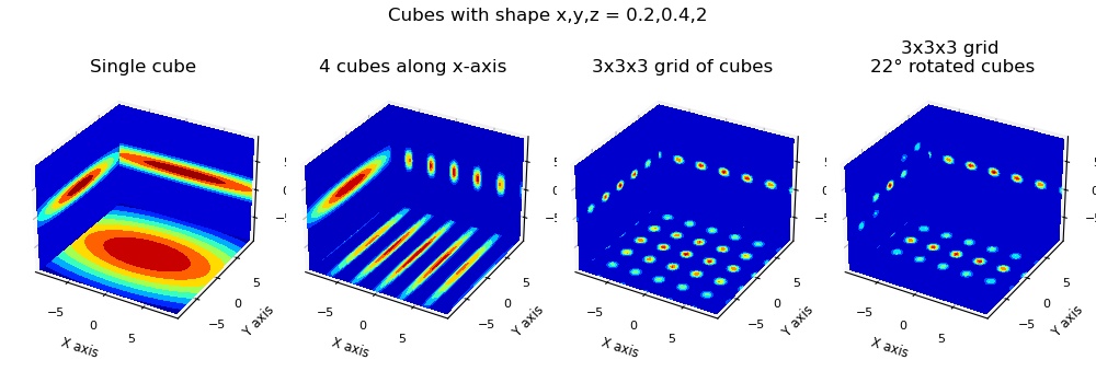
The same as above with 20° average disorder in orientation
`dorient=np.deg2rad(20)`leading to smearing of high Q patterns.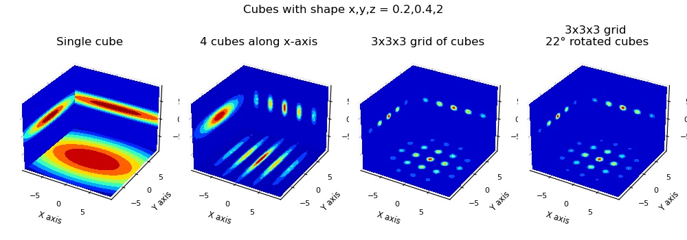
Build tetraeders of spheres and position on simple grid 3x3x3 We depict the respective q=0 plane at the surface of a cube to present all 3 orientations.
import jscatter as js
import numpy as np
from scipy.spatial.transform import Rotation

# detector planes; a real flat detector has z>0
q = np.mgrid[-9:9:51j, -9:9:51j].reshape(2,-1).T
qz =np.c_[q,np.zeros_like(q[:,0])]  # for z=0
qy = (Rotation.from_euler('x',np.pi/2).as_matrix() @ qz.T).T
qx = (Rotation.from_euler('y',np.pi/2).as_matrix() @ qz.T).T

# a 3D scattering amplitude of a tetraeder of
N=20
R=np.linalg.norm(qz,axis=1).max()
grid= js.sf.scLattice(R/N,N).XYZ

# Tetraeder: 4 points on a unit sphere, centroid at the origin, with lower face level, edge length = sqrt(8/3)
tetraeder = np.zeros([4,3])
tetraeder[0]=np.r_[(8/9)**0.5,0,-1/3]
tetraeder[0]=np.r_[-(2/9)**0.5, (2/3)**0.5,-1/3]
tetraeder[0]=np.r_[-(2/9)**0.5,-(2/3)**0.5,-1/3]
tetraeder[0]=np.r_[0,0,1]
V=4/3*np.pi*((8/3)**0.5 * 0.2)**3  # 0.2* edge length
fa = js.ff.orientedCloudScattering(grid[:,:3],cloud=tetraeder,formfactoramp='sphere',V=V)[[0,1,2,4]].array.T

# a small lattice of 3x3x3 cubes
cub27 = js.lattice.scLattice(2,[1,1,1]).points
cub27 = np.hstack([cub27,np.zeros([cub27.shape[0],2])])
ffz27 = js.ff.orientedCloudScattering3Dff(qz,cloud=cub27, formfactoramp=fa)
ffy27 = js.ff.orientedCloudScattering3Dff(qy,cloud=cub27, formfactoramp=fa)
ffx27 = js.ff.orientedCloudScattering3Dff(qx,cloud=cub27, formfactoramp=fa)

# show as cube surfaces
ax = js.mpl.contourOnCube(ffz27[[0,1,3]].array,ffx27[[1,2,3]].array,ffy27[[0,2,3]].array,offset=[-9,-9,9])
ax.figure.suptitle('Tetraders in 3x3x3 cubic lattice')
ax.figure.tight_layout()
#ax.figure.savefig(js.examples.imagepath+'/cloudTetraders.jpg')
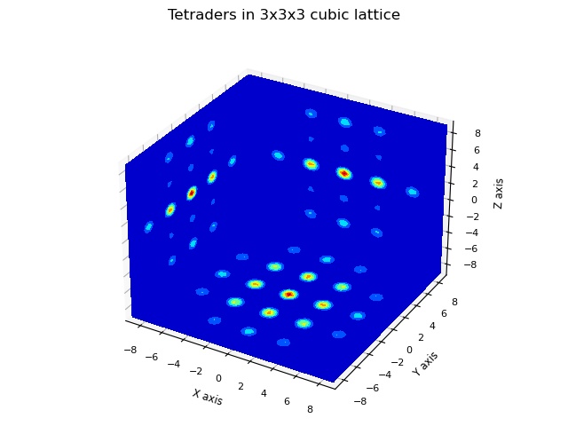
Look at the calculated formfactor of a single particle
import jscatter as js
import numpy as np
# detector plane (z=0 will be added automatically), for real flat detector z will be small but !=0)
qxzw = np.mgrid[-5:5:51j, -7:7:71j].reshape(2,-1).T

# create a grid for the formfactor amplitude fa larger than maximum detector q.
N=20
R=np.linalg.norm(qxzw,axis=1).max()
grid= js.sf.scLattice(R/N,N).XYZ #
# formfactor amplitude with edge length a,b,c in xyz direction
fa = js.ff.fa_cuboid(*grid[:,:3].T,0.31,3.141,0.31)

# look at formfactor amplitude
x,y,z,Y = fa[fa[:,2]==0].T
figfa = js.mpl.surface(x,y,Y)
figfa.axes[0].set_title(r'formfactor amplitude $F_a$ with negative values')

# to look at a single particle
rod0=np.array([[0,0,0,1,0,0]])
ffe=js.ff.orientedCloudScattering3Dff(qxzw,cloud=rod0, formfactoramp=fa)
fig=js.mpl.surface(ffe.X,ffe.Z,ffe.Y)
fig.axes[0].set_title(r'formfactor $F_a^2$')
fig.show()
- jscatter.ff.ornsteinZernike(q, xi, I0=1)[source]
Lorenz function, Ornstein Zernike model of critical systems.
The models is also used to describe diffuse scattering.
- Parameters:
- qarray
Wavevectors in units 1/nm
- xifloat
Correlation length
- I0float
scale
- Returns:
- dataArray [q, Iq]
Notes
A spatial correlation of the form
\[\rho(r)_{OZ}= \frac{\rho_0}{r}e^{-\frac{r}{\xi}}\]results in the scattering intensity
\[I(q) = \frac{I_0}{1+q^2\xi^2}\]A detailed explanation is found in [2].
References
[1]Accidental deviations of density and opalescence at the critical point of a single substance. Ornstein, L., & Zernike, F. (1914). Proc. Akad. Sci.(Amsterdam), 17(September), 793–806. Retrieved from http://www.dwc.knaw.nl/DL/publications/PU00012727.pdf
[2]Correlation functions and the critical region of simple fluids. Fisher, M. E. (1964). Journal of Mathematical Physics, 5(7), 944–962. https://doi.org/10.1063/1.1704197
[3]Origin of the scattering peak in microemulsions Teubner, M.; Strey, R. Chem. Phys. 1987, 87 (5), 3195–3200 DOI: 10.1063/1.453006
- jscatter.ff.pearlNecklace(Q, N, Rc=None, l=None, A1=None, A2=None, A3=None, ms=None, mr=None, vmonomer=None, monomerlength=None)[source]
Formfactor of a pearl necklace (freely jointed chain of pearls connected by rods)
The formfactor is normalized to 1. With no pearls we have connected rods, with no rods we have connected pearls.
- Parameters:
- Qarray
Wavevector in nm.
- Rcfloat
Pearl radius in nm. For Rc==0 forces ms=0.
- Nfloat
Number of pearls (homogeneous spheres).
- lfloat
Physical length of the rods in nm
- A1, A2, A3float
Amplitudes of pearl-pearl, rod-rod and pearl-rod scattering. Can be calculated with the number of chemical monomers in a pearl ms and rod mr (see below for further information) If ms and mr are given A1,A2,A3 are calculated from these.
- msfloat, default None
Number of chemical monomers in each pearl.
- mrfloat, default None
Number of chemical monomers in rod like strings.
- vmonomerfloat
Monomer specific volume \(v_0\) in cubic nm. Used to calculate Rc as \(Rc= (\frac{ms v_03}{4\pi})^{1/3}\). Increasing vmonomer compard to the bulk simulates swelling due to solvent inclusion.
- monomerlengthfloat
Monomer length a in nm to calculate \(l=m_r a\).
- Returns:
- dataArray
- Columns [q, Iq]
.pearlRadius
.A1 = ms²/(M*mr+N*ms)²
.A2 = mr²/(M*mr+N*ms)²
.A3 = (mr*ms)/(M*mr+N*ms)²
.numberPearls N
.numberRods M = (N-1) number of rod like strings
.mr
.ms
.stringLength
.numberMonomers : \(Nm_s + Mm_r\)
Notes
For absolute scattering see introduction formfactor (ff).
For Rc==0 we have no pearls, but we have a necklace of linear linkers like connected infinitely thin rods.
One finds (see [1] for equ. numbering)
\[I(Q) = \frac{(S_{ss}(Q)+S_{rr}(Q)+S_{rs}(Q))} {(M m_r + N m_s)^2} ; equ. 12\]with (s = sphere; r=thin rod; M=N-1)
\[S_{ss}(Q) = 2m_s^2F_a^2(Q)\left[\frac{N}{1-sin(Ql)/Ql}-\frac{N}{2}- \frac{1-(sin(Ql)/Ql)^N}{(1-sin(Ql)/Ql)^2}\cdot\frac{sin(Ql)}{Ql}\right] ; equ. 13\]\[S_{rr}(Q) = m_r^2\left[M\left\{2\Lambda(Q)-\left(\frac{sin(Ql/2)}{Ql/2}\right)\right\}+ \frac{2M\beta^2(Q)}{1-sin(Ql)/Ql}-2\beta^2(Q)\cdot \frac{1-(sin(Ql)/Ql)^M}{(1-sin(Ql)/Ql)^2}\right] ; equ. 13\]\[S_{rs}(Q) = m_r m_s \beta (Q) F_a (Q) \cdot 4\left[ \frac{N-1}{1-sin(Ql)/Ql}-\frac{1-(sin(Ql)/Ql)^{N-1}}{(1-sin(Ql)/Ql)^2} \cdot \frac{sin(Ql)}{Ql}\right] ; equ. 18\]and with formfactor amplitudes for a sphere \(F_a(Q) = 3 (sin(QR)-QR cos(QR))/(QR)^3\) and for rods (different ends) \(\Lambda(Q) = (\int_0^{Ql}\frac{sin(t)}{t}dt)/(Ql) ; (equ. 16)\) and \(\beta(Q) = (\int_{QR}^{Q(A-R)}\frac{sin(t)}{t}dt/(Ql) ; (equ. 17)\)
Author: L. S. Fruhner, RB, FZJ Juelich 2016
References
[1]Particle scattering factor of pearl necklace chains R. Schweins, K. Huber, Macromol. Symp., 211, 25-42, 2004. https://doi.org/10.1002/masy.200450702 https://ur.booksc.me/dl/21367099/4f9118
Examples
The formfactor describes a short necklace e.g. from magnetic nanoparticles building a chain or spheres connected by bonds. In the graph the modulations in mid Q range are interferences between neighboring beads.
import jscatter as js
import numpy as np
q=js.loglist(0.01,5,300)
p=js.grace()
for l in [2,20,50]:
    p.plot(js.ff.pearlNecklace(q, Rc=2, N=5, ms=200-l, mr=l,monomerlength=0.1),le='l=$stringLength mr=$mr')
p.yaxis(scale='l',label='I(q)',min=0.0003,max=1.1)
p.xaxis(scale='l',label='q / nm\S-1')
p.legend(x=0.2,y=0.01)
p.title('pearl necklace with 5 pearls')
p.subtitle('increasing string length reducing pearls')
# p.save(js.examples.imagepath+'/pearlNecklace.jpg')
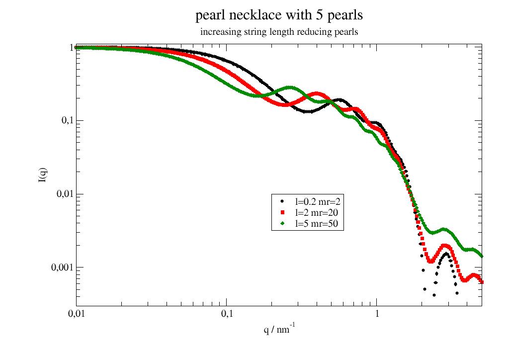
- jscatter.ff.polygon(q, L=3, R=0.3, n=30, N=3, V=None, formfactoramp='sphere', rms=0, ffpolydispersity=0, relError=100)[source]
2D Polygon as triangle, square, pentagon, circle build from beads along the segments.
Think e.g. about DNA origami… returns normalized formfactor.
- Parameters:
- qarray, 1xN or 3xN
Scattering vector in units 1/nm. If 1 dim array the spherical average is returned. For 3xN array as xyz coordinates no average is performed (for 2D images).
- Lfloat
Side length in unit nm.
- Rfloat
Radius of the sides in nm.
- Nint
- Number of sides in polygon.
3 trinagle
4 square
5 pentagon
n
- nfloat
Number of beads per side
- Vfloat
Volume of scatteres. If None a volume of \(4/3\piR^3\) with R =L/n (touching spheres) is assumed.
- formfactorampNone,’gauss’,’sphere’, ‘coil’
Normalized scattering amplitudes of cloud points. None means == 1. See
cloudScattering()- rmsfloat
Root mean square displacement of the positions as random (Gaussian) displacements in nm. See
cloudScattering()- ffpolydispersityfloat
Polydispersity of the points. See
cloudScattering()- relErrorfloat
See
cloudScattering()for meaning.
- Returns:
- dataArraynormalized formfactor
dinside inside diameter \(d_i=L cot(\pi/n)\)
doutside outside diameter \(d_i=L csc(\pi/n)\)
Notes
Just the geometric shape of polygons filled with beads.
With a large number of beads and formfactoramp==None after calculation a disc like shape can be multiplied. (see wormlikechain).
Examples
Trinagle, square, hexagon and circle of about same countour length. Number and size of beads similar.
import jscatter as js
import numpy as np
q = js.loglist(0.01,6,300)
contour=60
ff = None # 'sphere'
triangle = js.ff.polygon(q, L=contour/3, n=contour/3, N=3,formfactoramp=ff, relError=150)
square = js.ff.polygon(q, L=contour/4, n=contour/4, N=4,formfactoramp=ff, relError=150)
hexagon = js.ff.polygon(q, L=contour/6, n=contour/6, N=6,formfactoramp=ff, relError=150)
circle = js.ff.polygon(q, L=contour/20, n=contour/20, N=20,formfactoramp=ff, relError=150)

p = js.grace(1.5,1.5)
p.plot(triangle.X,triangle.Y,le='triangle')
p.plot(square.X,square.Y,le='square')
p.plot(hexagon.X,hexagon.Y,le='hexagon')
p.plot(circle.X,circle.Y,le='circle20')
p.yaxis(scale='log',label='F(Q)')
p.xaxis(scale='log',label=r'Q / nm\S-1')
p.legend(x=0.02,y=0.3)
p.title('Polygons')
p.subtitle('same contour length and approximate bead size')

p.new_graph( xmin=0.2,xmax=0.6,ymin=0.2,ymax=0.46)
for N in [3,4,6,20]:
   points = js.ff.polygonPoints(L=contour/N,n=contour/N,N=N)
   p[1].plot(points.T)
p[1].xaxis(label='',min=-10,max=20)
p[1].yaxis(label='',min=-0,max=20)

# p.save(js.examples.imagepath+'/polygons.jpg',size=(2,2))
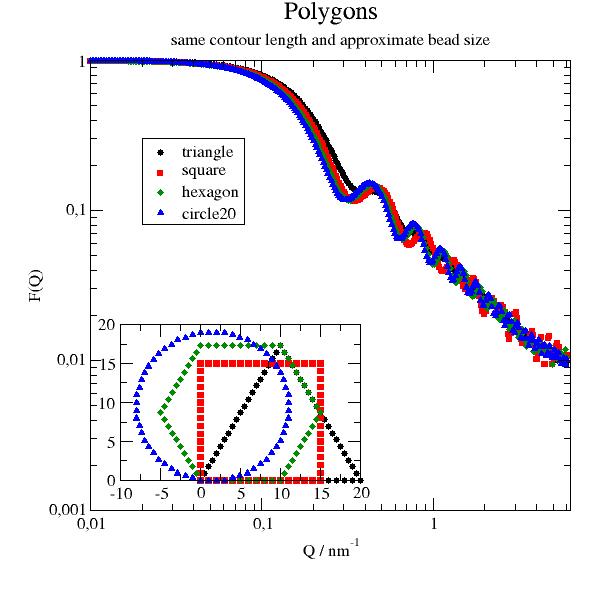
- jscatter.ff.polymerCorLength(q, xi, m, I0=1)[source]
Polymer scattering switching from collapsed over theta solvent to good solvent including chain overlap.
- Parameters:
- qarray
Wavevectors in units 1/nm
- xifloat
Correlation length
- mfloat
Porod exponent describing high q power law. m is related to Flory excluded volume exponent 𝜈 as m=1/𝜈 m=2 is Lorentz function (Ornstein-Zernike critical system)
- I0float
scale
- Returns:
- dataArray [q, Iq]
Notes
According to [1] the polymer scattering in solution can be described by the correlation length xi using:
\[I(q) = \frac{I_0}{1+(q\xi)^m} \ with \ m=1/\nu\]For collapsed chain 𝜈=1/3 ; m=3
For theta solvent 𝜈=1/2 ; m=2
For good solvent 𝜈=3/5 ; m=5/3
For Rg one finds \(R_g^2 = \frac{b^2N^{2\nu}}{(2\nu+1)(2\nu+2)}\). For details see [1] and [2].
References
[1] (1,2)Insight Into Chain Dimensions in PEO/Water Solutions B. HAMMOUDA, D. L. Ho, Journal of Polymer Science, Part B: Polymer Physics, 45(16), 2196–2200. https://doi.org/10.1002/polb.21221
[2]Insight into Clustering in Poly(ethylene oxide) Solutions B. Hammouda,* D. L. Ho, and S. Kline, Macromolecules 2004, 37, 6932-6937, doi: 10.1021/ma049623d
- jscatter.ff.powerLaw(q, d, A)[source]
Power law function / Porod scattering
\[F(q) = Aq^{-d}\]- Parameters:
- qarray
Wavevector in 1/nm.
- dfloat
Power law exponent or Porod exponent.
- Afloat
Amplitude
- Returns:
- dataArray
Notes
For flat interfaces (surfaces) Porod predict a \(q^{-4}\) behavior at larger q (only this is Porod scattering). This was later extended to rough surfaces by Sinha et al.[R0e1fb24dc17f-1]_ for fractal surfaces.
Similar is found for mass fractal aggregates.
The power law function is often used to represent the high q scattering representing different structures when the Q range to low Q is limited that details for more specific models are missing. The different power laws are connected to :
d = 5/3-2 swollen polymer chains,
d = 2 ideal Gaussian chains
d > 2 compacted polymer chain
d = 3 globular e.g. collapsed chains. (volume scattering)
d = 4 surface scattering at a sharp interface/surface (Porod scattering)
d = 6-dim rough surface area with a dimensionality dim between 2-3 (rough surface)
d < 3 mass fractals
The naming of the power law regions is not clear to me (different from the Guinier region which is well defined). While the Porod law for flat surfaces is d=4, sometimes its called the Porod exponent [2] or fractal exponent. A Porod region is connected to a region with d=4 or the region of Porod analysis (plot I*q^4 vs. q) and for d<4 a fractal region is observed. Often Porod region is used as synonymous for “high Q power law region” which is not necessarily connected to Porod scattering.
For q=0 the function is undefined
References
[1]X-ray and neutron scattering from rough surfaces S. K. Sinha, E. B. Sirota, S. Garoff, and H. B. Stanley Phys. Rev. B 38, 2297 (1988) https://doi.org/10.1103/PhysRevB.38.2297
[2]Analysis of the Beaucage model Boualem Hammouda J. Appl. Cryst. (2010). 43, 1474–1478 http://dx.doi.org/10.1107/S0021889810033856
- jscatter.ff.prism(q, R, H, SLD=1, solventSLD=0, relError=300)[source]
Formfactor of prism (equilateral triangle) .
- Parameters:
- qarray 3xN
- Rfloat
Edge length of equilateral triangle in units nm.
- Hfloat
Height in units nm
- SLDfloat, default =1
Scattering length density unit nm^-2 e.g. SiO2 = 4.186*1e-6 A^-2 = 4.186*1e-4 nm^-2 for neutrons
- solventSLDfloat, default =0
Scattering length density of solvent. unit nm^-2 e.g. D2O = 6.335*1e-6 A^-2 = 6.335*1e-4 nm^-2 for neutrons
- relErrorfloat, default 300
- Determines how points on sphere are selected for integration
>=1 Fibonacci Lattice with relError*2+1 points (min 15 points)
- 0<1 Pseudo random points on sphere (see randomPointsOnSphere).
Stops if relative improvement in mean is less than relError (uses steps of 20*ncpu new points). Final error is (stddev of N points) /sqrt(N) as for Monte Carlo methods. even if it is not a correct 1-sigma error in this case.
- Returns:
- dataArray [q, fq]
Notes
With contrast \(\rho\) and wavevector \(q=[q_x,q_y,q_z]\) the scattering amplitude \(F_a(q)\) is
\[F_a(q_x,q_y,q_z) = \rho \frac{2 \sqrt{3} e^{-iq_yR/ \sqrt{3}} H} {q_x (q_x^2-3q_y^2)} \ (q_x e^{i q_yR\sqrt{3}} - q_xcos(q_xR) - i\sqrt{3} q_ysin(q_xR)) sinc(q_zH/2)\]and \(F(q)=<F_a(q)F^*_a(q)>=<|F_a(q)|^2>\)
References
[1]DNA-Nanoparticle Superlattices Formed From Anisotropic Building Blocks Jones et al Nature Materials 9, 913–917 (2010), doi: 10.1038/nmat2870
Examples
import jscatter as js
q = js.loglist(0.1,5,100)
p = js.grace()
fq = js.ff.prism(q,3,3)
p.plot(fq.X,fq.Y/fq.I0)
p.yaxis(scale='log')
- jscatter.ff.raftDecoratedCoreShell(q, Rcore, Rraft, Nraft, coreSLD, raftSLD, shellthickness=None, shellSLD=None, solventSLD=0, distribution='fibonacci', dR=0.2, dRraft=0.1, ndrop=7, relError=100, cmap='hsv', show=False)[source]
Scattering of multiCoreShell particle decorated with disc-like rafts in the shell.
- The model described a multiCoreShell particle decorated with discs.
Discs are only located in the shells describing e.g. liposomes with patches of different lipids or proteins.
- Parameters:
- qarray
Wavevectors in units 1/nm.
- Rcorefloat
Core radius in nm.
- shellthicknessfloat or list of float
Thickness of consecutive shells from core to outside in units nm. Might be zero.
- shellSLDfloat or list of float
Scattering length of consecutive shells corresponding to shellthickness. Unit is nm^-2
- raftSLDfloat or list of float
Scattering length of raft in unit nm^-2.
- Rraftfloat,
Radius of small rafts or discs decorating the shell in units nm.
- dRraftfloat,
Relative polydispersity of raft radius.
- Nraftint
Number of rafts on shell.
- coreSLDfloat
Scattering length of core in unit nm^-2.
- solventSLDfloat
Solvent scattering length density in unit nm^-2.
- distribution‘fibonacci’,’quasirandom’
- Distribution of rafts as :
- ‘fibonacci’ A Fibonacci lattice on the sphere with Nraft points.
For even Nraft the point [0,0,1] is removed
- ‘quasirandom’ quasirandom distribution of Nraft rafts on sphere surface.
The distribution is always the same if repeated several times.
- dRfloat, default 0.1
Fluctuation of Rcore (or shellthickness[0] if rcore=0). This radius polydispersity suppresses the strong minima of a multishell structure at high q and reduce there depth at low Q to get a more realistic pattern. Rafts are scaled along radius changing their radius keeping the SLD and the raft surface fraction constant.
- ndropint
Number of points in grid on length sum(shellthickness). Determines resolution of the droplets. Large ndrop increase the calculation time by ndrop**3. To small give wrong scattering length contributions in shell and core.
- relErrorfloat
Determines calculation method. See
cloudScattering()- showbool
Show a 3D image using matplotlib.
- cmapmatplotlib colormap name
Only for show to determine the colormap. See js.mpl.showColors() for all possibilities.
- Returns:
- dataArray
- Columns [q, Fq, Fq coreshell]
attributes from call
.SurfaceFraction \(=N_{raft}R_{raft}^2/(4(R_{core} + shellthickness + H_{raft})^2)\)
Notes
- The models uses cloudscattering with multi component particle distribution.
At the center is a multiShellSphere with core and shell located.
At the positions of a disc a grid of small particles describe the respective shape as disc.
Each particle gets a respective scattering length to result in the correct scattering length density including the overlap with the central core-shell particle.
cloudscattering is used to calculate the respective scattering including all cross terms.
If discs overlap the overlap volume is only counted once. For large Nraft the raft layer might be full, check .SurfaceFraction. In this case the disc represents the shell, while the rafts represent still some surface roughness. Rraft is explicitly not limited to allow this.
As described in cloudscattering for high q a bragg peak will appear showing the particle bragg peaks. This is far outside the respective SAS scattering. The validity of this model is comparable to A nano cube build of different lattices. For higher q the ndrop resolution parameter needs to be increased.
References
[1]How cholesterol stiffens unsaturated lipid membranes S. Chakraborty et al. PNAS, 117, 21896-21905 (2020), https://doi.org/10.1073/pnas.200480711
[2]Areas of Monounsaturated Diacylphosphatidylcholines. Kučerka N, et al. (2009) Biophys. J. 97(7):1926-1932.
Examples
Lipid rafts on liposome A multiCoreShell with discs can describe lipid rafts (e.g. cholesterol or another lipid) on a liposome. The outer shells may have solventSLD to allow a disc of larger thickness compared to the central shell. The disc SLD in raftSLD are choosen to mimic a raft of longer lipid tails due to addtion of cholesterol.
SLD and tail/head thickness according to [1] and [2].
import jscatter as js
import numpy as np
q=js.loglist(0.01,5,300)

# thickness of head and tail region of lipid bilayer
st = [0.5,0.5,2.8,0.5,0.5]
# corresponding contrast
fe = js.formel.felectron
sSLD = 335 * fe  # H2O unit e/nm³*fe
sld = np.r_[sSLD, 495* fe,280* fe,495* fe, sSLD]  # unit e/nm³*fe
dSLD = np.r_[495*fe, 280*fe, 280*fe, 280*fe, 495*fe]
Rraft = 8

fig = js.ff.raftDecoratedCoreShell(q=q,Rcore=50, Rraft=Rraft, Nraft=20, dR=3,ndrop=7, cmap='prism',
                coreSLD=sSLD, shellthickness=st, shellSLD=sld, raftSLD=dSLD, solventSLD=sSLD, show=1)

bb=fig.axes[0].get_position()
fig.axes[0].set_title('rafts on liposome')
fig.axes[0].set_position(bb.shrunk(0.5,0.9))
ax1=fig.add_axes([0.58,0.1,0.4,0.85])

raft = js.ff.raftDecoratedCoreShell(q=q,Rcore=50, Rraft=Rraft, Nraft=20, dR=3, ndrop=7,
                coreSLD=sSLD, shellthickness=st, shellSLD=sld, raftSLD=dSLD, solventSLD=sSLD, show=0)

ax1.plot(raft.X, raft._cs_fq,'--', label='liposome without raft')
ax1.plot(raft.X, raft.Y,           label='lot lipid rafts on liposome')

raft2 = js.ff.raftDecoratedCoreShell(q=q,Rcore=50, Rraft=Rraft, Nraft=3, dR=3, ndrop=7,
                coreSLD=sSLD, shellthickness=st, shellSLD=sld, raftSLD=dSLD, solventSLD=sSLD, show=0)
ax1.plot(raft2.X, raft2.Y, label='few lipid rafts on liposome')

raft2 = js.ff.raftDecoratedCoreShell(q=q,Rcore=50, Rraft=Rraft*0.5, Nraft=3, dR=3, ndrop=7,
                coreSLD=sSLD, shellthickness=st, shellSLD=sld, raftSLD=dSLD, solventSLD=sSLD, show=0)
ax1.plot(raft2.X, raft2.Y, label='few small lipid rafts on liposome')

ax1.set_yscale('log')
ax1.set_xscale('log')
ax1.legend()
fig.set_size_inches(8,4)
# fig.savefig(js.examples.imagepath+'/liposome_with_raft.jpg')
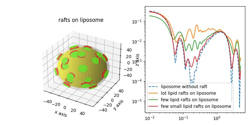
- jscatter.ff.ringORZ(q, N=100, l=1, fa=None)[source]
Formfactor of a ring polymer using optimized Rouse-Zimm approximation (ORZ).
The ring chain is described within the more general optimized Rouse-Zimm (ORZ) approximation introduced by Bixon and Zwanzig [3] [4] . See
solveOptimizedRouseZimm().We extend this here using bead scattering lengths for partial matching. Currently uncorrelated bonds.
- Parameters:
- qarray
Scattering vectors in units 1/nm.
- Nint
Number of beads .
- lfloat, default = 0.38 nm (amino acid)
Bond length or Kuhn length in units nm.
- faNone, list of float
Scattering length of bead/monomer \(fa_i\). Can be used to match parts of the star to the solvent.
None : Equal 1 for all beads.
list: length N as scattering length of beads in sequence
- Returns:
- fqdataArray
Formfactor a linear chain.
[q; fq]
columnname = ‘q;fq’
.l : bondlength l
.N : Number of beads
.Rg : radius of gyration in nm
.Rg_red : reduced radius of gyration
Notes
See
solveOptimizedRouseZimm()for a description of the ORZ model with respective parameters.Here we use a ring chain with N beads of uncorrelated beads with costheta=0 .
The structural matrix has diagonal elements, \(A_{ii}=2\) and \(A_{i\neq j}=-1\) if the ith and jth monomers are connected to each other or zero otherwise.
References
[1]Static and Dynamic Structure Factors for Star Polymers in θ Conditions. Guenza, M. & Perico, A. Macromolecules 26, 4196–4202 (1993). https://doi.org/10.1021/ma00068a020
[2]A Local Approach to the Dynamics of Star Polymers. Guenza, M., Mormino, M. & Perico, A. Macromolecules 24, 6168–6174 (1991). https://doi.org/10.1021/ma00023a018
[3]Theoretical basis for the Rouse‐Zimm model in polymer solution dynamics. Zwanzig, R. The Journal of Chemical Physics 60, 2717–2720 (1974) https://doi.org/10.1063/1.1681433
[4]A hierarchy of models for the dynamics of polymer chains in dilute solution. Perico, A., Ganazzoli, F. & Allegra, G. The Journal of Chemical Physics 87, 3677–3686 (1987). https://doi.org/10.1063/1.452966
Examples
Here we examine how changig stiffness influences the form factor.
import jscatter as js
import numpy as np

q= js.loglist(0.02,5,100)

p = js.grace()
p.multi(2,1)

for c,l in enumerate(np.r_[0.5:2:3j],1):
    fq = js.ff.ringORZ(q, N=100, l=l, fa=None)
    p[0].plot(fq,li=[1,1,c],sy=0,le=f'Rg={fq.Rg:.2f} nm\\S-1')
    # Kratky plot
    p[1].plot(fq.X,fq.Y*fq.X**2,li=[1,1,c],sy=0,le=f'Rg={fq.Rg:.2f} nm\\S-1')

p[0].xaxis(label='',scale='log')
p[1].xaxis(label='q / nm\S-1')
p[0].yaxis(label='I(Q)',scale='log',min=100,max=20000)
p[1].yaxis(label='I(Q)Q\S2',scale='norm',min=0.01,max=2000)
p.title('ringORZ')
p[1].text('Kratky plot',x=0.5,y=1700)
p[0].legend(x=0.02,y=6000,charsize=0.6)
# p.save(js.examples.imagepath+'/ORZ_ring_ff.png',size=(1.5,1.5),dpi=300)
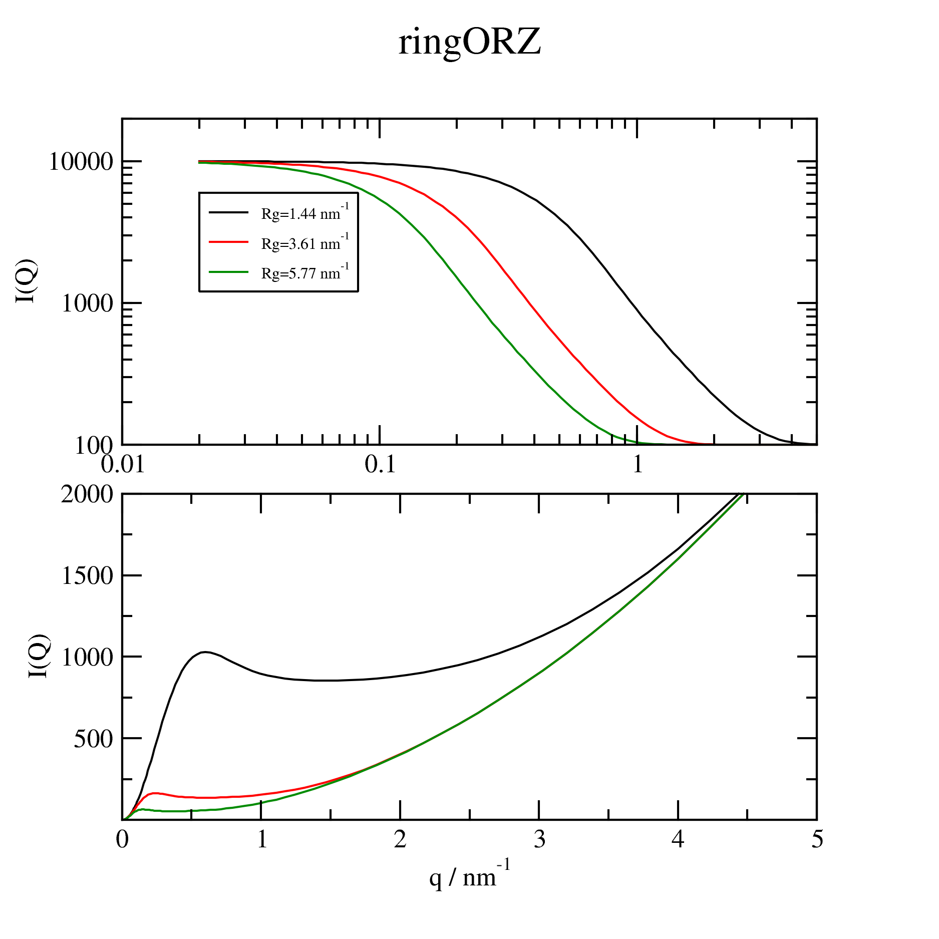
- jscatter.ff.ringPolymer(q, N=None, a=None, Rg=None, nu=0.5)[source]
General formfactor of a polymer ring with excluded volume effects.
- Parameters:
- qarray
Scattering vector, unit e.g. 1/A or 1/nm
- afloat, default =1
Segment length in nm.
- Ninteger
Number of segments
- Rgfloat
Radius of gyration, units in 1/unit(q)
- nufloat, default=0.5
ν is the excluded volume parameter, which is related to the Porod exponent d as ν = 1/d and [5/3 <= d <= 3].
fully swollen chains ν = 3/5 (good solvent)
for Gaussian chains ν = 1/2 (theta solvent)
collapsed chains ν = 1/3 (bad solvent)
- Returns:
- dataArray
- Columns [q,Fq]
.segmentlength segment length a
.N number of segments
.Rg radius of gyration
.nu excluded volume parameter
Notes
Equ 52 in [1]
\[F(q) = 2\int_0^1 ds(1-s) e^{-q^2a^2N^{2\nu}s^{2\nu}(1-s^{2\nu})/6}\]with \(R_g^2=\frac{a^2N^{2\nu}}{2}\frac{3\nu}{1+7\nu+14\nu^2+8\nu^3}\)
For nu=0.5 equ. 3.5 in [2] shows in short form related to the Dawson function
\[S(Q) = dawsn(U)/U = \frac{e^{-U^2}}{U} \int_0^U e^{t^2}\]with \(U=(q^2R_{g,l}^2)^{1/2}/2\) for \(R_{g,l}\) from the linear chain (not Rg of the ring!).
For \(nu=0.5\) the familiar result is recovered \(R_g^2 = a^2 N / 12 =\frac{1}{2} R^2_[g,linear]\) .
References
[1]Form Factors for Branched Polymers with Excluded Volume Boualem Hammouda Journal of Research of the National Institute of Standards and Technology 121,139 (2016) http://dx.doi.org/10.6028/jres.121.006
[2]Some statistical properties of flexible ring polymers Edward F. Casassa JOURNAL OF POLYMER SCIENCE: PART A, 3, 605-614 (1965) https://doi.org/10.1002/pol.1965.100030217
Examples
The excluded volume effects with \(\nu \neq 0.5\) lead to increase/decrease at high q in the Kratky representation compared to nu=0.5 of a theta solvent.
import jscatter as js
import numpy as np
q=js.loglist(0.03,8,100)
p=js.grace(1.4,1)
p.multi(1,2)

for nu in [0.4,0.45,0.5,0.55,0.6]:
    iq=js.ff.ringPolymer(q,Rg=5,nu=nu)
    p[0].plot(iq,le=f'nu={nu:.2f} N={iq.N:.0f} Rg={iq.Rg:.1f}')
    p[1].plot(iq.X*iq.Rg, iq.Y*iq.X**2,le=f'{nu}')

p[0].yaxis(scale='l',label='I(q) / a.u.')
p[0].xaxis(scale='l',label='q / nm\S-1')
p[1].yaxis(scale='l',label=[r'I(q)q\S2\N / a.u.',1,'opposite'],ticklabel=['power',0,1,'opposite'],min=1e-2,max=0.2)
p[1].xaxis(scale='l',label=r'qR\sg\N ')
p[0].legend(x=0.03,y=0.01)
p[1].subtitle('Kratky plot')
p[0].title('ring polymer')
p[0].subtitle('Rg = 5 nm, a=1')
#p.save(js.examples.imagepath+'/ringPolymer.jpg',size=(1.4,1))
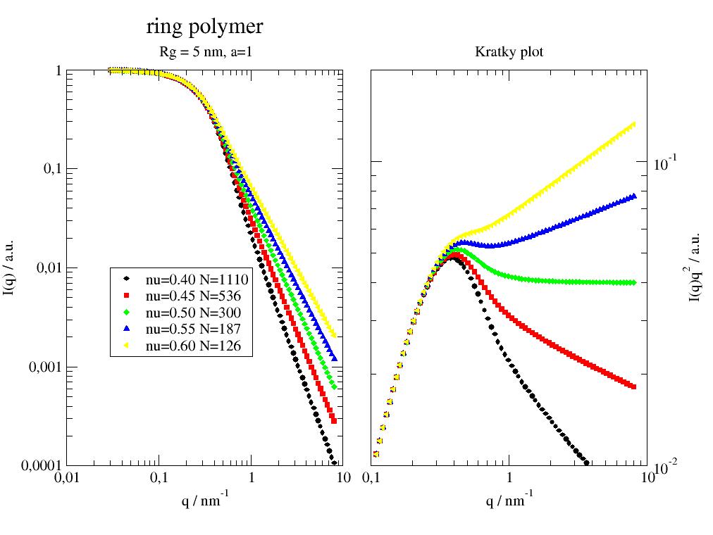
- jscatter.ff.sphere(q, radius, contrast=1)[source]
Scattering of a single homogeneous sphere.
- Parameters:
- qfloat
Wavevector in units of 1/nm
- radiusfloat
Radius in units nm
- contrastfloat, default=1
Difference in scattering length to the solvent = contrast
- Returns:
- dataArray
Columns [q, Iq, fa] Iq scattering intensity - fa formfactor amplitude - .I0 forward scattering
Notes
\[I(q)= \rho^2V^2\left[\frac{3(sin(qR) - qR cos(qR))}{(qR)^3}\right]^2\]with contrast \(\rho\) and sphere volume \(V=\frac{4\pi}{3}R^3\)
The first minimum of the form factor is at qR=4.493
References
[1]Guinier, A. and G. Fournet, “Small-Angle Scattering of X-Rays”, John Wiley and Sons, New York, (1955).
Examples
import jscatter as js
import numpy as np
q=js.loglist(0.1,5,300)
p=js.grace()
R=3
sp=js.ff.sphere(q, R)
p.plot(sp.X*R,sp.Y,li=1)
p.yaxis(label='I(q)',scale='l',min=1e-4,max=1e5)
p.xaxis(label='qR',scale='l',min=0.1*R,max=5*R)
p.legend(x=0.15,y=0.1)
#p.save(js.examples.imagepath+'/sphere.jpg')
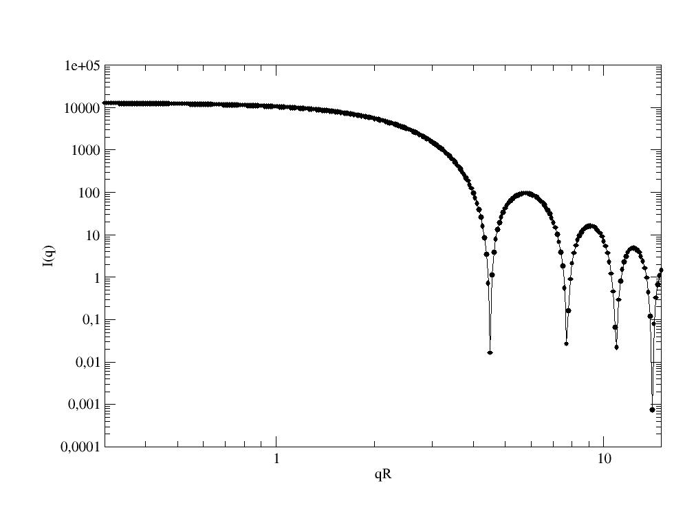
- jscatter.ff.sphereCoreShell(q, Rc, Rs, bc, bs, solventSLD=0)[source]
Scattering of a spherical core shell particle.
See multiShellSphere.
- Parameters:
- qfloat
Wavevector in units of 1/(R units)
- Rc,Rsfloat
Radius core and radius of shell Rs>Rc
- bc,bsfloat
Contrast to solvent scattering length density of core and shell.
- solventSLDfloat, default =0
Scattering length density of the surrounding solvent. If equal to zero (default) then in profile the contrast is given.
- Returns:
- dataArray
Columns [wavevector ,Iq, fa]
Examples
import jscatter as js
q=js.loglist(0.01,5,500)
p=js.grace()
FF=js.ff.sphereCoreShell(q,6,12,-0.2,1)
p.plot(FF,sy=[1,0.2],li=1)
p.yaxis(label='I(q)',scale='l',min=1,max=1e8)
p.xaxis(label='q / nm\S-1',scale='l')
#p.save(js.examples.imagepath+'/sphereCoreShell.jpg')
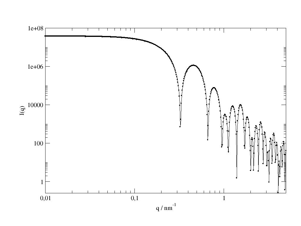
- jscatter.ff.sphereCoreShellGaussianCorona(q, Rc, Rs, Ncoil, Nmonomer, monomerVolume, a, coilSLD, coreSLD, shellSLD, nu=0.5, solventSLD=0, d=1)[source]
Scattering of a core-shell particle surrounded by gaussian coils as model for grafted polymers on particle.
The model is in analogy to the sphereGaussianCorona replacing the sphere by a core shell particle in [1]. The additional scattering from the coils is uniformly distributed at the surface, which might fail for lower aggregation numbers as 1, 2, 3. Instead of aggregation number equ. 1 in [1] we use volume of the gaussian coils collapsed to the surface.
- Parameters:
- q: array of float
Wavevectors in unit 1/nm.
- Rc,Rsfloat
Radius of core and shell in unit nm.
- dfloat, default 1
Coils centre located d*Rg away from the sphere surface This might be equivalent to Rg
- Ncoilfloat
Number of coils at the surface (aggregation number)
- Nmonomerint
Monomer number in single ring.
- afloat
Monomer segment length in units nm.
- monomerVolumefloat
Monomer volume in unit nm³.
- nufloat, default=0.5
ν is the excluded volume parameter (see gaussianChain), which is related to the Porod exponent d as ν = 1/d and [5/3 <= d <= 3].
fully swollen chains ν = 3/5 (good solvent)
for Gaussian chains ν = 1/2 (theta solvent)
collapsed chains ν = 1/3 (bad solvent)
- coilSLDfloat
Scattering length density of coil in bulk as if collapsed on surface unit nm^-2.
- coreSLD,shellSLDfloat, default see text
Scattering length density of core and shell in unit nm^-2.
- solventSLDfloat, default 0
Scattering length density of solvent. unit nm^-2.
- Returns:
- dataArray
- Columns [q,Iq]
.coilRg
.Radii
.numberOfCoils
.coildistancefactor
.coilequVolume
.coilSLD
.coreshellSLD
.solventSLD
Notes
See
sphereGaussianCorona()and exchange sphere score by coreshell ff.Rg=N**0.5*b with N monomers of length b
Vcoilsphere=N*monomerVolume=4/3.*np.pi*coilequR**3
coilequR=(N*monomerVolume/(4/3.*np.pi))**(1/3.)
References
[1] (1,2)Form factors of block copolymer micelles with spherical, ellipsoidal and cylindrical cores Pedersen J Journal of Applied Crystallography 2000 vol: 33 (3) pp: 637-640
[2]Hammouda, B. (1992).J. Polymer Science B: Polymer Physics30 , 1387–1390
Examples
Example for silica particle coated with something and additional polymer coils.
import jscatter as js
q=js.loglist(0.1,5,100)
p=js.grace(1.4,1)
p.multi(1,2)
for rsld, ssld, le in [[1e-4,4e-4,'mixed contrast'],
                       [6e-4,4e-4,'matched coil'],
                       [1e-4,6e-4,'matched core']]:
   fq = js.ff.sphereCoreShellGaussianCorona(q,Rc=2,Rs=2,Ncoil=10,Nmonomer=166,monomerVolume=0.3,a=0.8,
                       coilSLD=rsld,coreSLD=0.9*ssld, shellSLD=1.1*ssld, solventSLD=6e-4)
   p[0].plot(fq, le=le)
   # Kratky plot
   p[1].plot(fq.X*fq.coilRg,fq.Y*fq.X**2 *1e4)
p[0].plot(fq.X,fq.Ncoil * fq._Iqcoil,le='pure coils')
p[1].plot(fq.X*fq.coilRg,fq.Ncoil * fq._Iqcoil*fq.X**2 *1e4)

p[0].yaxis(label='I(q)', charsize=1.5,scale='l',min=1e-7,max=0.001)
p[0].xaxis(label=r'q / nm\S-1',scale='l')
p[1].yaxis(label=[r'I(q)q\S2\N / a.u.',1.5,'opposite'],scale='n',min=0,max=0.38)
p[1].xaxis(label=r'q R\sg',scale='n')

p[0].legend(x=0.2,y=1e-6)
# p.save(js.examples.imagepath+'/sphereCoreShellGaussianCorona.jpg',size=(1.4,1),dpi=600)
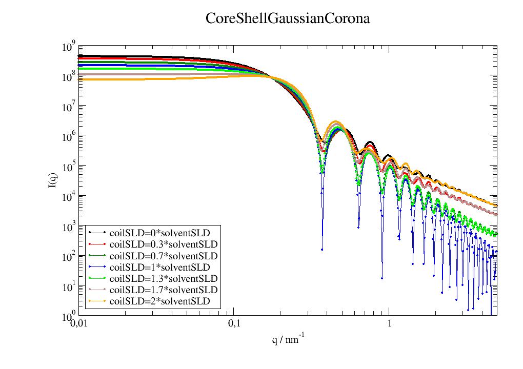
- jscatter.ff.sphereFuzzySurface(q, R, sigmasurf, contrast)[source]
Scattering of a sphere with a fuzzy interface.
- Parameters:
- qfloat
Wavevector in units of 1/(R units)
- Rfloat
The particle radius R represents the radius of the particle where the scattering length density profile decreased to 1/2 of the core density.
- sigmasurffloat
Sigmasurf is the width of the smeared particle surface.
- contrastfloat
Difference in scattering length to the solvent = contrast
- Returns:
- dataArray
Columns [q, Iq] Iq scattering intensity related to sphere volume. - .I0 forward scattering
Notes
A radial box profile (H(r-R) Heaviside function) is convoluted with a Gaussian to smear the edge.
\[\rho(r) \propto H(r-R)\circledast e^{-\frac{1}{2}r^2\sigma_{surf}^2}\]The convolution results in the multiplication of the sphere formfactor amplitude with a gaussian leading to
\[I(q)= 4\pi\rho^2V^2[F_a(q)]^2\]\[F_a(q)= \frac{3(sin(qR) - qr cos(qR))}{(qR)^3} e^{-\frac{1}{2}q^2\sigma_{surf}^2}\]with contrast \(\rho\) and sphere volume \(V=\frac{4\pi}{3}R^3\).
The “fuzziness” of the interface is defined by the parameter sigmasurf (width of the Gaussian). The particle radius R represents the radius of the particle where the scattering length density profile decreased to 1/2 of the core density. sigmasurf is the width of the smeared particle surface. The inner regions of the microgel that display a higher density are described by the radial box profile extending to a radius of approximately Rbox ~ R - 2(sigma). In dilute solution, the profile approaches zero as Rsans ~ R + 2(sigma).
References
[1]Stieger, J. S. Pedersen, P. Lindner, W. Richtering, Langmuir 20 (2004) 7283-7292
Examples
import jscatter as js
import numpy as np
q=js.loglist(0.1,5,300)
p=js.grace()
sFS=js.ff.sphereFuzzySurface(q, 3, 0.01, 1)
p.plot(sFS,le='sigmasurf=0.01')
sFS=js.ff.sphereFuzzySurface(q, 3, 0.5, 1)
p.plot(sFS,le='sigmasurf=0.3')
sFS=js.ff.sphereFuzzySurface(q, 3, 1, 1)
p.plot(sFS,le='sigmasurf=1')
p.yaxis(label='I(q)',scale='l',min=1e-4,max=1e5)
p.xaxis(label='q / nm\S-1',scale='l')
p.legend(x=0.15,y=0.1)
#p.save(js.examples.imagepath+'/sphereFuzzySurface.jpg')
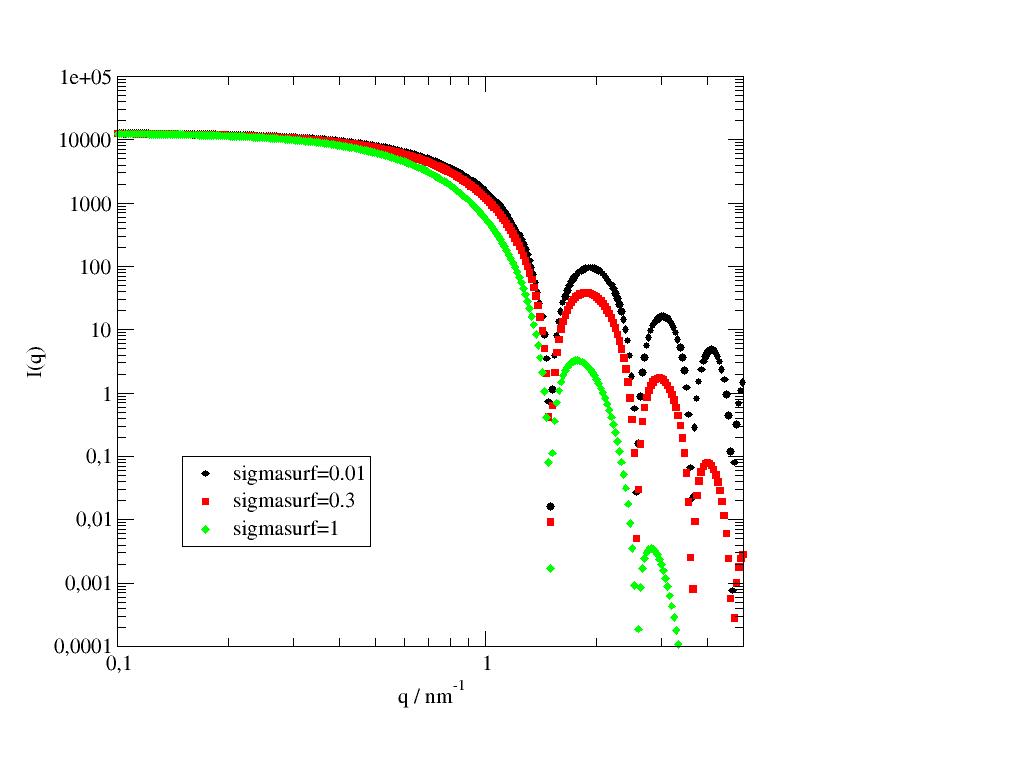
- jscatter.ff.sphereGaussianCorona(q, R, Ncoil, Nmonomer, monomerVolume, a, nu=0.5, coilSLD=6.4e-05, sphereSLD=0.0004186, solventSLD=0.0006335, d=1)[source]
Scattering of a sphere surrounded by gaussian coils as model for grafted polymers on particle e.g. a micelle.
The additional scattering is uniformly distributed at the surface, which might fail for lower aggregation numbers as 1, 2, 3. Alternativly wormlike chains can be used.
- Parameters:
- q: array of float
Wavevectors in unit 1/nm
- Rfloat
Sphere radius in unit nm
- dfloat, default 1
Coils centre located d*Rg away from the sphere surface
- Ncoilfloat
Number of coils at the surface (aggregation number)
- Nmonomerint
Monomer number in single ring.
- afloat
Monomer segment length in units nm.
- monomerVolumefloat
Monomer volume in unit nm³.
- nu0<float<1, default=0.5, None
ν is the excluded volume parameter (see gaussianChain), which is related to the Porod exponent d as ν = 1/d and [5/3 <= d <= 3].
fully swollen chains ν = 3/5 (good solvent)
for Gaussian chains ν = 1/2 (theta solvent)
collapsed chains ν = 1/3 (bad solvent)
None : Use
wormlikeChain()
- coilSLDfloat
Scattering length density of coil in bulk \(\rho_{coil}\). unit nm^-2. default hPEG = 0.64*1e-6 A^-2 = 0.64*1e-4 nm^-2
- sphereSLDfloat
Scattering length density of sphere.unit nm^-2. default SiO2 = 4.186*1e-6 A^-2 = 4.186*1e-4 nm^-2
- solventSLDfloat
Scattering length density of solvent. unit nm^-2. default D2O = 6.335*1e-6 A^-2 = 6.335*1e-4 nm^-2
- Returns:
- dataArray
- Columns [q,Iq]
.coilRg
.sphereRadius
.Ncoil
.coildistancefactor
.coilequVolume
.coilSLD
.sphereSLD
.solventSLD
Notes
We calc in analogy to [1]
\[\begin{split}F(Q) &= F_{sphere}(Q,R) \\ &+ N_{coil} F_{coil}(Q, Rg,\nu) \\ &+ 2N_{coil} F_{a,sphere}(Q,R) F_{a,coil}(Q,Rg,\nu) sin(Q(R + d R_g))/(Q(R + d R_g)) \\ &+ N_{coil} * (N_{coil} - 1) F_{coil}(Q, R_g,\nu) (sin(Q(R + d R_g)) / (Q(R + d R_g)))^2\end{split}\]with formfactors \(F(Q,)=F^2_a(Q,)\) of a sphere \(F_{sphere}(Q,R)\) and the coils \(F_{coil}(Q,R,\nu)\)
The formfactor amplitudes
\[\begin{split}F_{a,sphere}(Q,R) &= \rho_{sphere} V_{sphere}\left[\frac{3(sin(qR) - qR cos(qR))}{(qR)^3}\right] \\ F_{a,coil}(Q,R_g,\nu) &= \rho_{coil} V_{coil} (F_{coil}(Q,R_g,\nu))^{0.5}\end{split}\]with the generalized Gaussian chain \(F_{coil}(Q)\) (see
gaussianChain())\[F_{coil}(Q) = \frac{1}{\nu U^{\frac{1}{2\nu}}} \gamma_{inc}(\frac{1}{2\nu}, U) - \frac{1}{\nu U^{\frac{1}{\nu}}} \gamma_{inc}(\frac{1}{\nu}, U)\]with \(U=R^2_g Q^2\) and \(\gamma_{inc}\) as lower incomplete gamma function, sphere volume V and contrast \(\rho\).
Explicitly we use the root of the GaussianChain formfactor for a coil formfactor amplitude. The in some papers mentioned \(\frac{1-exp(-x)}{x}\) for Debye function (see references) is only valid for QRg<<1 and results in the wrong high Q limit. This is not immediately visible as the \(Q^{-2}\) at high Q results from the second dominating term. The generalized Gaussian F(Q) is always positive and does not cross zero.
- The defaults values result in a silica sphere with hPEG grafted at the surface in D2O.
Rg=N**0.5*b with N monomers of length b
Vcoilsphere=N*monomerVolume=4/3.*np.pi*coilequR**3
coilequR=(N*monomerVolume/(4/3.*np.pi))**(1/3.)
References
[1]Form factors of block copolymer micelles with spherical, ellipsoidal and cylindrical cores Pedersen J. Journal of Applied Crystallography 2000 vol: 33 (3) pp: 637-640
[2]Hammouda, B. (1992). J. Polymer Science B: Polymer Physics30 , 1387–1390
Examples
import jscatter as js
q=js.loglist(0.1,5,100)
p=js.grace(1.4,1)
p.multi(1,2)
for rsld, ssld, le in [[1e-4,4e-4,'mixed contrast'],
                       [6e-4,4e-4,'matched coil'],
                       [1e-4,6e-4,'matched core']]:
   fq = js.ff.sphereGaussianCorona(q,R=4,Ncoil=10,Nmonomer=66,monomerVolume=0.12,a=0.8,
                       coilSLD=rsld,sphereSLD=ssld, solventSLD=6e-4)
   p[0].plot(fq, le=le)
   # Kratky plot
   p[1].plot(fq.X*fq.coilRg,fq.Y*fq.X**2 *1e4)
p[0].plot(fq.X,fq.Ncoil * fq._Iqcoil,le='pure coils')
p[1].plot(fq.X*fq.coilRg,fq.Ncoil * fq._Iqcoil*fq.X**2 *1e4)

p[0].yaxis(label='I(q)', charsize=1.5,scale='l',min=1e-6,max=0.1)
p[0].xaxis(label=r'q / nm\S-1',scale='l')
p[1].yaxis(label=[r'I(q)q\S2\N / a.u.',1.5,'opposite'],scale='n',min=0,max=3.5)
p[1].xaxis(label=r'q R\sg',scale='n')

p[0].legend(x=0.7,y=0.03)
#p.save(js.examples.imagepath+'/sphereGaussianCorona.jpg',size=(1.4,1),dpi=600))

- jscatter.ff.superball(q, R, p, SLD=1, solventSLD=0, nGrid=12, returngrid=False)[source]
A superball is a general mathematical shape that can be used to describe rounded cubes, sphere and octahedron’s.
The shape parameter p continuously changes from star, octahedron, sphere to cube.
- Parameters:
- qarray
Wavevector in 1/nm
- Rfloat, None
2R = edge length
- pfloat, 0<p<100
- Parameter that describes shape
p=0 empty space
p<0.5 concave octahedron’s
p=0.5 octahedron
0.5<p<1 convex octahedron’s
p=1 spheres
p>1 rounded cubes
p->inf cubes
- SLDfloat, default =1
Scattering length density of cuboid. unit nm^-2
- solventSLDfloat, default =0
Scattering length density of solvent. unit nm^-2
- nGridint
Number of gridpoints in superball volume is ~ nGrid**3. The accuracy can be increased increasing the number of grid points dependent on needed q range. Orientational average is done with 2(nGrid*4)+1 orientations on Fibonacci lattice.
- returngridbool
Return only grid as lattice object. The a visualisation can be done using grid.show()
- Returns:
- dataArray
Columns [q,Iq, beta]
Notes
The shape is described by
\[|x|^{2p} + |y|^{2p} + |z|^{2p} \le |R|^{2p}\]which results in a sphere for p=1. The numerical integration is done by a pseudorandom grid of scatterers.
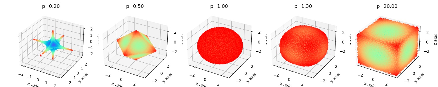
References
[1]Periodic lattices of arbitrary nano-objects: modeling and applications for self-assembled systems Yager, K.G.; Zhang, Y.; Lu, F.; Gang, O. Journal of Applied Crystallography 2014, 47, 118–129. doi: 10.1107/S160057671302832X
Examples
Visualisation as shown above
import jscatter as js
import numpy as np
import matplotlib.pyplot as plt
from mpl_toolkits.mplot3d import Axes3D
fig = plt.figure(figsize=[15,3])
q=np.r_[0:5:0.1]
R=3
for i,p in enumerate([0.2,0.5,1,1.3,20],1):
    ax = fig.add_subplot(1,5,i, projection='3d')
    grid=js.ff.superball(q,R,p=p,nGrid=40,returngrid=True)
    grid.filter(lambda xyz: np.linalg.norm(xyz))
    grid.show(fig=fig, ax=ax,atomsize=0.2)
    ax.set_title(f'p={p:.2f}')
#fig.savefig(js.examples.imagepath+'/superballfig.jpg')
Compare to extreme cases of sphere (p=1) and cube (p->inf , use here 100) to estimate the needed accuracy in your Q range.
import jscatter as js
import numpy as np
#
q=np.r_[0:3.5:0.02]
R=6
nGrid=25
p=js.grace()
p.multi(2,1)
p[0].yaxis(scale='l',label='I(q)')
ss=js.ff.superball(q,R,p=1,nGrid=12)
p[0].plot(ss,legend='superball p=1 nGrid=12 default')
ss=js.ff.superball(q,R,p=1,nGrid=25)
p[0].plot(ss,legend='superball p=1 nGrid=25')
p[0].plot(js.ff.sphere(q,R),li=1,sy=0,legend='sphere ff')
p[0].legend(x=2,y=5e5)
#
p[1].yaxis(scale='l',label='I(q)')
p[1].xaxis(scale='n',label='q / nm\S-1')
cc=js.ff.superball(q,R,p=100)
p[1].plot(cc,sy=[1,0.3,1],legend='superball p=100 nGrid=12')
cc=js.ff.superball(q,R,p=100,nGrid=25)
p[1].plot(cc,sy=[1,0.3,2],legend='superball p=100 nGrid=25')
p[1].plot(js.ff.cuboid(q,2*R),li=4,sy=0,legend='cuboid')
p[1].legend(x=2,y=9e5)
p[0].title('Superball with transition from sphere to cuboid')
p[0].subtitle('p=1 sphere; p>1 round cube; p>20 cube  ')
#p.save(js.examples.imagepath+'/superball.jpg')
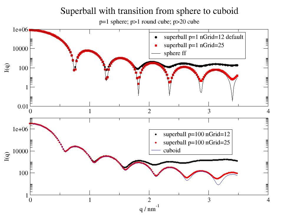
Superball scaling with \(q/p^{1/3}\) close to sphere shape with p=1. Small deviations from sphere (as a kind of long wavelength roughness) cannot be discriminated from polydispersity or small ellipsoidality.
import jscatter as js
import numpy as np
q=np.r_[0:5:0.02]
R=3

Fq=js.dL()
for i,p in enumerate([0.5,0.8,0.9,1,1.115,1.3,2],1):
    fq=js.ff.superball(q,R,p=p,nGrid=20)
    Fq.append(fq)

pp=js.grace()
pp.multi(2,1,vgap=0.2)
for fq in Fq[1:-1]:
    pp[0].plot(fq.X,fq.Y/fq.Y[0],sy=[-1,0.2,-1],le=f'{fq.rounding_p:.2g}')
    pp[1].plot(fq.X*fq.rounding_p**(1/3),fq.Y/fq.Y[0],sy=[-1,0.2,-1],le=f'{fq.rounding_p:.2g}')
fq=Fq[0]
pp[0].plot(fq.X,fq.Y/fq.Y[0],sy=0,li=[1,2,-1],le=f'{fq.rounding_p:.2g}')
pp[1].plot(fq.X*fq.rounding_p**(1/3),fq.Y/fq.Y[0],sy=0,li=[1,2,-1],le=f'{fq.rounding_p:.2g}')
fq=Fq[-1]
pp[0].plot(fq.X,fq.Y/fq.Y[0],sy=0,li=[3,2,-1],le=f'{fq.rounding_p:.2g}')
pp[1].plot(fq.X*fq.rounding_p**(1/3),fq.Y/fq.Y[0],sy=0,li=[3,2,-1],le=f'{fq.rounding_p:.2g}')

pp[0].legend(x=0.2,y=0.05)
pp[0].yaxis(label='I(q)',scale='l')
pp[1].yaxis(label='I(q)',scale='l')
pp[0].xaxis(label='q / nm')
pp[1].xaxis(label=r'q/p\S1/3\N')
pp[0].title('superball scaling')
pp[0].subtitle('p=0.5 octahedron, p=1 sphere, p>10 cube')
pp[1].text(r'q scaled by p\S-1/3\nclose to p=1 I(q) scales to similar shape ',x=4,y=0.1)
pp[0].text('original',x=4,y=0.1)
#p.save(js.examples.imagepath+'/superballscaling.jpg')
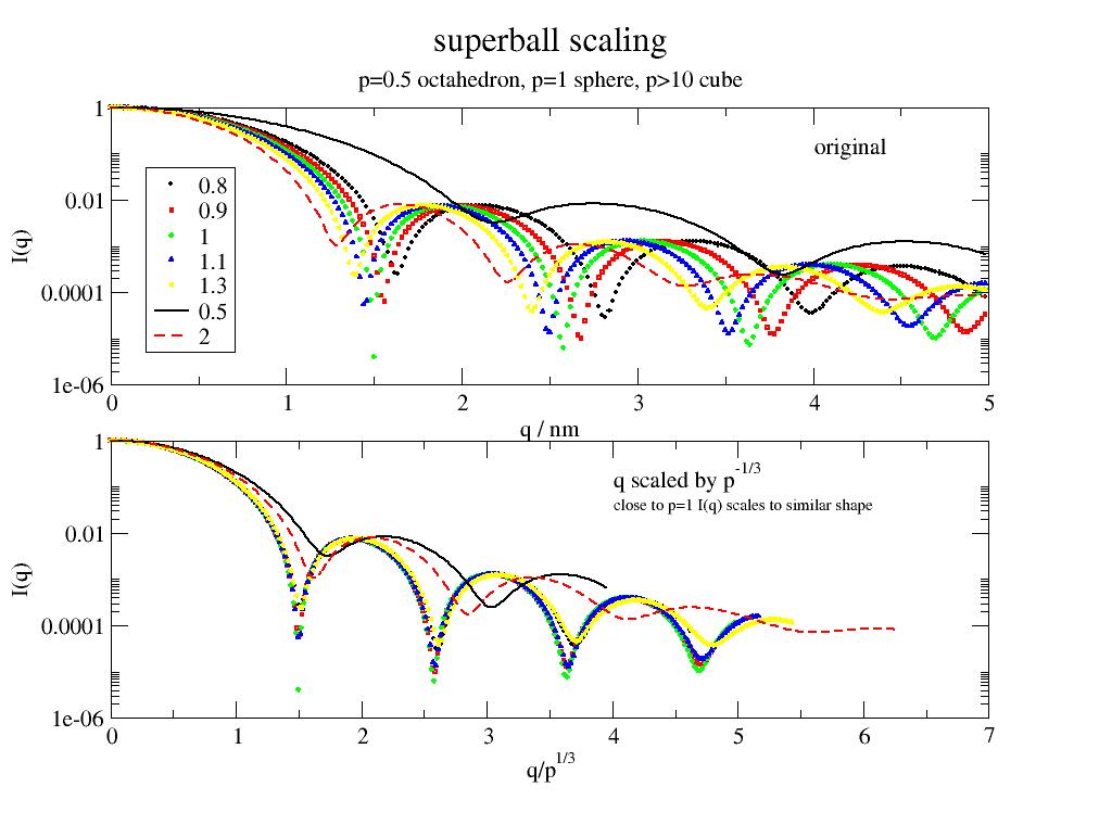
- jscatter.ff.teubnerStrey(q, xi, d, eta2=1)[source]
Scattering from space correlation ~sin(2πr/D)exp(-r/ξ)/r e.g. disordered bicontinious microemulsions.
Phenomenological model for the scattering intensity of a two-component system using the Teubner-Strey model [1]. Often used for bi-continuous micro-emulsions.
- Parameters:
- qarray
Wavevectors
- xifloat
Correlation length
- dfloat
Characteristic domain size, periodicity.
- eta2float, default=1
Squared mean scattering length density contrast \(\eta^2\)
- Returns:
- dataArray
Columns [q, Iq]
Notes
A correlation function \(\gamma(r) = \frac{d}{2\pi r}e^{-r/\xi}sin(2\pi r/d)\) yields after 3D Fourier transform the scattering intensity of form
\[I(q) = \frac{8\pi\eta^2/\xi}{a_2 + 2bq^2 + q^4}\]- with
\(k = 2 \pi/d\)
\(a_2 = (k^2 + \xi^{-2})^2\)
\(b = k^2 - \xi^{-2}\)
\(q_{max}=((2\pi/d)^2-\xi^{-2})^{1/2}\)
References
[1]M. Teubner and R. Strey, Origin of the scattering peak in microemulsions, J. Chem. Phys., 87:3195, 1987
[2]K. V. Schubert, R. Strey, S. R. Kline, and E. W. Kaler, Small angle neutron scattering near lifshitz lines: Transition from weakly structured mixtures to microemulsions, J. Chem. Phys., 101:5343, 1994
Examples
Teubner-Strey with background and a power law for low Q
import jscatter as js
import numpy as np

def tbpower(q,B,xi,dd,A,beta,bgr):
    # Model Teubner Strey  + power law and background
    tb=js.ff.teubnerStrey(q=q,xi=xi,d=dd)
    # add power law and background
    tb.Y=B*tb.Y+A*q**beta+bgr
    tb.A=A
    tb.bgr=bgr
    tb.beta=beta
    return tb

q=js.loglist(0.01,5,600)
p=js.grace()
data=tbpower(q,1,10,20,0.00,-3,0.)
p.plot(data,legend='no bgr, no power law')
data=tbpower(q,1,10,20,0.002,-3,0.1)
p.plot(data,legend='xi=10')
data=tbpower(q,1,20,20,0.002,-3,0.1)
p.plot(data,legend='xi=20')
p.xaxis(scale='l',label=r'Q / nm\S-1')
p.yaxis(scale='l',label='I(Q) / a.u.')
p.legend(x=0.02,y=1)
p.title('TeubnerStrey model with power law and background')
#p.save(js.examples.imagepath+'/teubnerStrey.jpg')
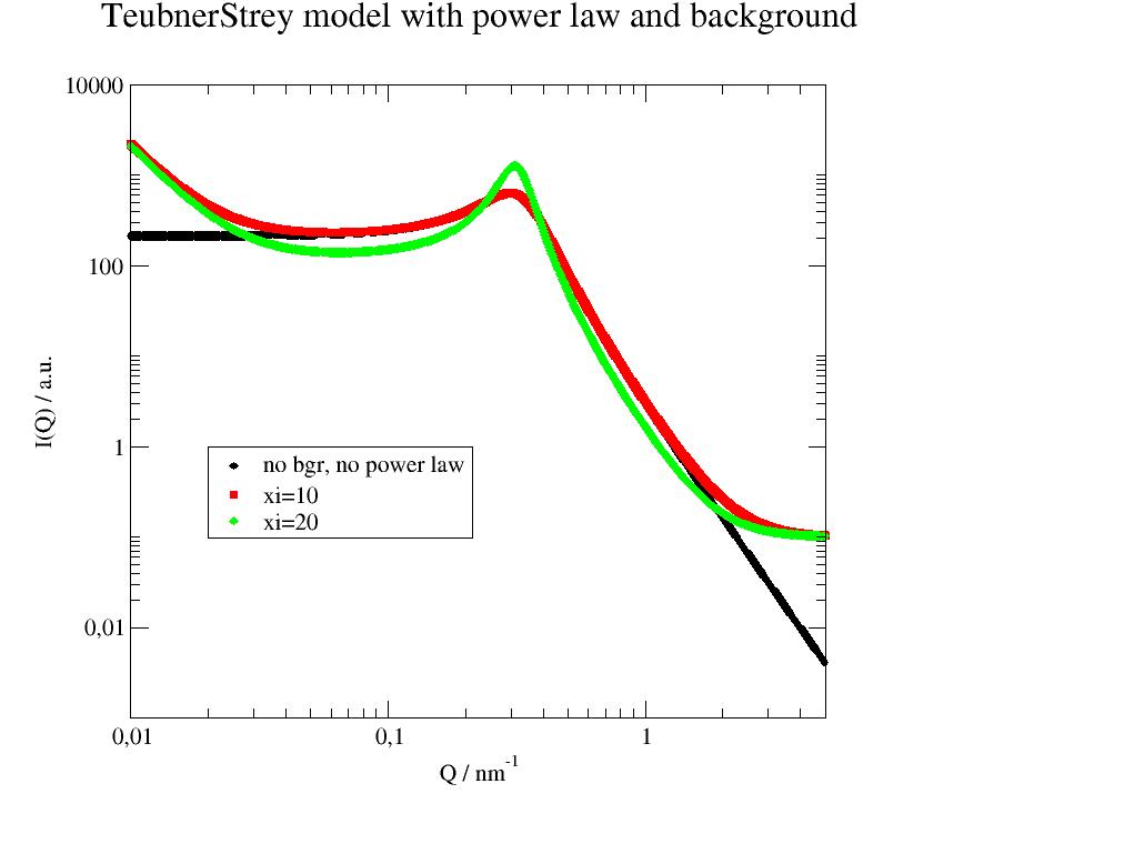
- jscatter.ff.triaxialEllipsoid(q, Ra, Rb, Rc, SLD=1, solventSLD=0, n=25)[source]
Formfactor triaxial ellipsoid.
- Parameters:
- qarray
Scattering vector in units 1/nm.
- Ra,Rb,Rcfloat
Half axes = radii in units nm.
- SLDfloat
Scattering length density in unit nm^-2.
- solventSLDfloat
Scattering length density of solvent in unit nm^-2 .
- nint
Order for Gaussian integration over both phi and theta.
- Returns:
- dataArray
- Columns [q; Iq]
.Ra, .Rb, .Rc
.volume
.I0 forward scattering q=0
Notes
According to [1] the triaxial ellipsoid is
\[I(q) = V^2 \rho^2 \int_0^{2\pi} \int_0^{\pi} \phi(QR_a)^2 sin(\theta) d\theta d\phi\]with \(u=QR_a\) and \(Q = (q_x^2 + (R_b/R_aq_y)^2 + (R_c/R_aq_z)^2 )^{(1/2)}\) and
\[\Phi(u) = \frac{3(sin(u)-u cos(u))}{u^3}\]also contrast \(\rho\), ellipsoid volume \(V = 4/3\pi R_a R_b R_c\)
References
[1]Generalizing small-angle scattering form factors with linear transformations Matt Thompson J. Appl. Cryst. (2020). 53, 1387-1391 https://doi.org/10.1107/S1600576720010389
Examples
Triaxial ellipsoid in vacuum
import jscatter as js
import numpy as np
q=np.r_[0.1:6:0.01]

p=js.grace()
elli = js.ff.triaxialEllipsoid(q,3,3,3)
p.plot(elli, sy=3, le='sphere')
p.plot(js.ff.sphere(q,radius=3),li=[1,2,1],sy=0)
# rotation ellipsoid
relli = js.ff.triaxialEllipsoid(q,3,4,4)
p.plot(relli, sy=2, le='rot ellipsoid')
p.plot(js.ff.ellipsoid(q,Ra=3,Rb=4),li=[1,2,1],sy=0)

telli = js.ff.triaxialEllipsoid(q,3,4,5)
p.plot(telli, sy=[3,0.2,3], le='triaxial ellipsoid')

p.yaxis(scale='l',label='I(q)',min=0.01,max=1e5)
p.xaxis(scale='l',label='q / nm\S-1',min=0.1,max=10)
p.legend(x=0.15,y=100)
p.title('triaxial ellipsoid model comparison ')
p.subtitle('lines are standard models for sphere and ellipsoid')
#p.save(js.examples.imagepath+'/triaxialEllipsoid(.jpg')

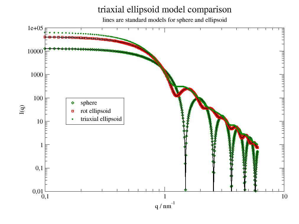
- jscatter.ff.wormlikeChain(q, N, a, R=None, SLD=1, solventSLD=0, rtol=0.02)[source]
Scattering of a wormlike chain, which correctly reproduces the rigid-rod and random-coil limits.
To calculate the scattering of the classical Kratky-Porod model of semiflexible chains we use an analytical solution for arbitrary stiffness and length as given by Kholodenko [1]. The transition from infinite thin chain to a cross sectional scattering uses the decoupling approximation and the scattering cross section of an infinitly thin (optional multishell)disc.
- Parameters:
- qarray
Wavevectors in 1/nm.
- Nfloat
Length of the chain in units nm. Number of chain segments is N/l=N/(2a). We follow here the notation of [1].
- afloat
Persistence length a with Kuhn length l=2a (segment length), units of nm.
- Rfloat, default None
- Radius of worm cross section in units of nm.
float : The volume is \(V = \piR^2 aN\) and a cylinder cross section is assumed.
None or <0 : Infinitly thin rod and normalized formfactor is returned. SLD ignored.
- SLDfloat
Scattering length density of segments.
- solventSLD
Solvent scattering length density.
- rtolfloat
Maximum relative tolerance in integration.
- Returns:
- dataArray
- Columns [q, Iq]
.chainRadius
.chainLength
.persistenceLength
.Rg
.volume
.contrast
.mu from \(Re =\sqrt{6} R_g = l (N/l)^\nu\)
For R=0 the normalized formfactor is returned.
Notes
We use equation 17 of [1] to calculate the normalized formfactor S(q) of a semiflexible thin polymer chain as it correctly recovers the limit of rigid rod and flexible chain (for details see [1]).
\[ \begin{align}\begin{aligned}S_{wc}(q) =& \frac{2}{x}[I_1(x)-\frac{1}{x}I_2(x)]\\with\; I_n =& \int_0^x z^{n-1}f(z) \; and \; x=\frac{3N}{2a}\\ k<=& 3/2a : \; f(z) = \frac{1}{E} \frac{sinh(Ez)}{sinh(z)}\\ k>& 3/2a : \; f(z) = \frac{1}{\overline{E}} \frac{sinh(\overline{E}z)}{sinh(z)}\\ E^2 =& 1-(\frac{2}{3}ak)^2 ;\; \overline{E}^2 = 1-(\frac{2}{3}ak)^2\end{aligned}\end{align} \]If the contour length is much larger than the cross section \(N>>R\) then the cross section scattering can be separated. Within a decoupling approximation [4] we may use an infinitly thin disc formfactor \(S_{disc}(q)\) oriented perpendicular to the chain. This can be calculated as homogeneous thin disc (included in using R>0) or as multi shell disc using multiShellDisc (see third example).
\[F(q) = S_{wc}(q,R=0,...) N S_{disc}(q,D=0,alpha=\pi/2,...)\]The forward scattering \(I_0\) for a homogeneous cylinder is \(I_0=V^2(SLD-solventSLD)^2\) with \(V=\pi R^2 N\). For multishellDisc(..,D=0,alpha=pi/2,..).I0 the result has to be multiplied by the contour length N.
.Rg is calculated according to equ 20 in [2] and similar is found in [3] with l=2a.
\[R_g^2 = \frac{lN}{6}\big( 1-\frac{3l}{2N}+\frac{3l^2}{2N^2}-\frac{3l^3}{4N^3}(1-e^{-2N/l}) \big)\]- From [1] :
The Kratky plot (Figure 4 ) is not the most convenient way to determine a as was pointed out in ref 20. Figure 5 provides an alternative way of measuring a by plotting the experimentally measurable combination Nk2S(k) versus a for fixed wavelength k. As Figure 5 indicates, this plot is rather insensitive to the chain length N and therefore is universal. The numerical analysis of eq 17 shows that this remains true for as long as k is not too small. Taking into account that the excluded-volume effects leave S(k) practically unchanged (e.g., see Figures 2 and 4 of ref 231, the plot of Figure 5 can serve as a useful alternative to the Kratky plot which, in addition, does not suffer from the polydispersity effects
References
[1] (1,2,3,4,5,6)Analytical calculation of the scattering function for polymers of arbitrary flexibility using the dirac propagator A. L. Kholodenko, Macromolecules, 26:4179–4183, 1993
[2]The structure factor of a wormlike chain and the random-phase-approximation solution for the spinodal line of a diblock copolymer melt Zhang X et. al. Soft Matter 10, 5405 (2014), https://doi.org/10.1039/C4SM00374H
[3]Models of Polymer Chains Teraoka I. in Polymer Solutions: An Introduction to Physical Properties pp: 1-67, New York, John Wiley & Sons, Inc. https://doi.org/10.1002/0471224510.ch1
Decoupling approximation for cross section
[4]Static structure factor of polymerlike micelles:Overall dimension, flexibility, and local properties of lecithin reverse micelles in deuterated isooctane Götz Jerke, Jan Skov Pedersen, Stefan Ulrich Egelhaaf, and Peter Schurtenberger Phys. Rev. E 56, 5772 ; https://doi.org/10.1103/PhysRevE.56.5772
Examples
Kratky and S(q) representation of the wormlike chain model showing the transition due to longer linear segments.
The longer the chain segments are the transition from Gaussian like \(~k^{-2}\) to local linear \(~k^{-1}\) shifts to smaller Q. The overall chain stays Gaussian like with a Flory size exponent \(\nu \approx 0.5\) .
import jscatter as js
p=js.grace()
p.multi(2,1)
p.title('figure 3 (2 scaled) of ref Kholodenko Macromolecules 26, 4179 (1993)',size=1)
q=js.loglist(0.01,10,100)
for a in [0.3,1,2.5,5,20,50]:
    ff=js.ff.wormlikeChain(q,200,a)
    p[0].plot(ff.X,200*ff.Y*ff.X**2,legend=f'a={ff.persistenceLength:.4g}; Rg={ff.Rg:.2g}; '+r'\xn\f{}='+f'{ff.mu:.2g}')
    p[1].plot(ff.X,ff.Y,legend=f'a={ff.persistenceLength:.4g}; Rg={ff.Rg:.2g}')
p[0].legend(x=11,y=30)
p[0].yaxis(label=r'Nk\S2\NS(k)')
p[0].xaxis(label='')
p[1].xaxis(label='k',scale='l')
p[1].yaxis(label='S(k)',scale='l')
p[1].text(r'~k\S-1',x=1,y=0.005)
p[1].text(r'~k\S-2',x=1,y=0.15)
#p.save(js.examples.imagepath+'/wormlikeChain.jpg')
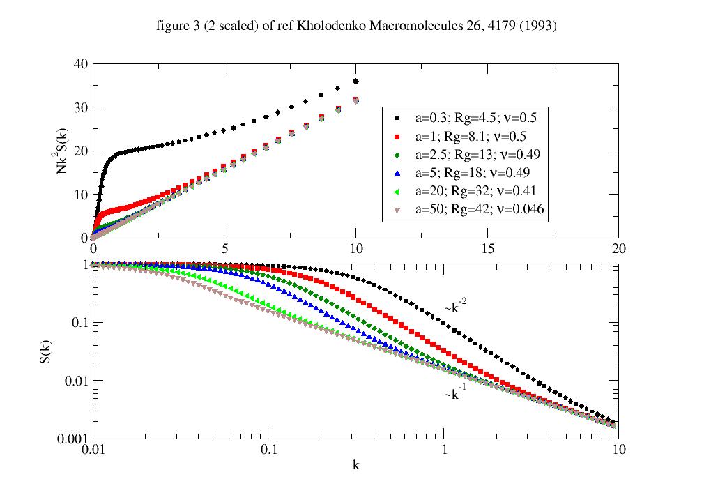
A rescaled version according to fig 3 of [1]
import jscatter as js
p=js.grace()
p.multi(2,1)
p.title('figure 4 of ref Kholodenko Macromolecules 26, 4179 (1993)',size=1)
# fig 4 seems to be wrong scale in [Rddefa3e3955e-1]_ as for large N with a=1 fig 2 and 4 should have same plateau.
a=1
q=js.loglist(0.01,4./a,100)
for NN in [1,20,50,150,500]:
    ff=js.ff.wormlikeChain(q,NN,a)
    p[0].plot(ff.X*a,NN*a*ff.Y*ff.X**2,legend='N=%.4g' %ff.chainLength)
    p[1].plot(ff.X,ff.Y,legend='a=%.4g' %ff.persistenceLength)
p[0].legend()
p[0].yaxis(label=r'(N/a)(ka)\S2\NS(k)')
p[0].xaxis(label='ka')
p[1].xaxis(label='k',scale='l')
p[1].yaxis(label='S(k)',scale='l')
Micellar wormlike structure with core shell disc cross section.
Instead of a core-shell disc multiShellDisc may approximate any radial distribution.
import jscatter as js
import numpy as np
def thickworm(q, N, a, Rcore, shellD, SLDcore=1, SLDshell=2, solventSLD=0):
   worm = js.ff.wormlikeChain(q, N, a, R=0)
   cross = js.ff.multiShellDisc(q, radialthickness=[Rcore,shellD], shellthickness=[0,0],
                               shellSLD=[SLDcore,SLDshell], solventSLD=solventSLD, alpha=np.pi/2)
   worm.Y = worm.Y*N*cross.Y
   worm.volume = N*np.pi*(Rcore+shellD)**2
   worm.I0 = cross.I0*N
   return worm

p=js.grace(1,0.7)
p.title('Thick wormlike chain with coreshell cross section',size=1.5)
p.subtitle('persistence length *a*')
q=js.loglist(0.01,4,200)
for a in [1,2.5,5,20,50]:
    ff=thickworm(q,N=200,a=a, Rcore=3, shellD=1, SLDcore=0, SLDshell=1)
    p.plot(ff.X,ff.Y,legend=f'a={ff.persistenceLength:.4g}; Rg={ff.Rg:.2g}')
p.legend(x=0.03,y=1000)
p.xaxis(label='q',scale='l',charsize=1.5)
p.yaxis(label='S(q)',scale='l',charsize=1.5,min=1,max=3e5)
#p.save(js.examples.imagepath+'/wormlikeChain2.jpg')
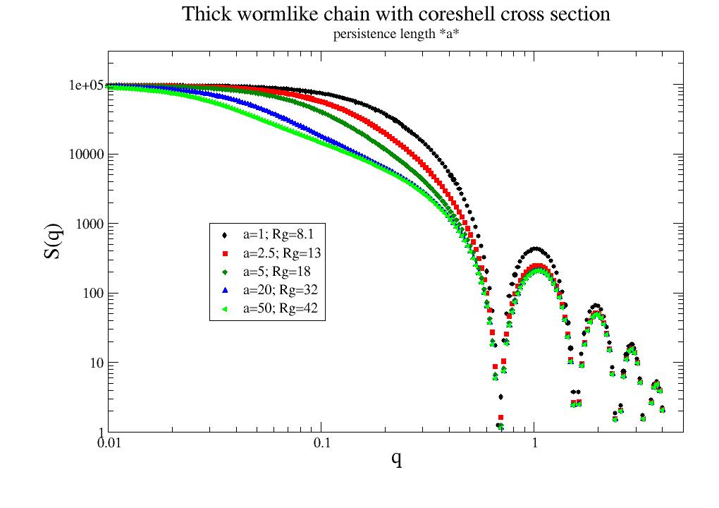
Cloud can represent any object described by a cloud of (different) scatterers with scattering amplitudes as constant, sphere scattering amplitude, Gaussian scattering amplitude or explicitly given ones.
The scattering of a cloud can represent the scattering of a cluster of particles with polydispersity and position distortion according to root-mean-square displacements (rms). Polydispersity and rms displacements are randomly changed within the explicit orientational average to represent an ensemble average (opposite to the time average of a single cluster).
The cloud can represent a particle lattice in a nano particle to describe the Bragg peaks or be used as a kind of volume integrations for arbitrary shaped particles. Additional complex objects composed of different types of subparticles can be created. E.g a hollow sphere decorated by Gaussian chains. See cloudscattering examples below.
The scattering is calculated by explicit calculation with a spherical average to allow inclusion of
polydispersity, position distortion and because it’s faster for large numbers of particles (>1000).
For small number of particles the Debye equation can be used but without polydispersity and position distortion.
See cloudScattering()
- Note:
Models that are build by positioning of differently shaped particles might depict approximations of the real scattering as overlaps are not considered or changes of specific configurations due to the presence of another particle might change. As an example we look at
sphereGaussianCorona(). The Gaussian coils have overlap with the inner sphere and for high aggregation numbers the coil overlap is not described correctly.Nevertheless, these approximations might be useful to describe general features of a scattering pattern. Additionally one might consider that analytic models as e.g. a sphere are approximations itself neglecting surface roughness, interfaces, deviations from symmetry or anisotropy and break down if a length scale of internal building blocks as e.g. atoms is reached.
Cloudscattering examples (Check the source as examples)
Cloudscattering results are normalized by \(I_0=(\sum b_i)^2\) to equal one for q=0 (except for polydispersity).
- jscatter.ff.cloudscattering.cloudScattering(q, cloud, relError=50, formfactoramp=None, V=None, rms=0, ffpolydispersity=0, ncpu=0)[source]
Orientation averaged scattering of a cloud of isotropic particles.
Cloud can represent any object/lattice described by a cloud of scatterers with scattering amplitudes as constant, sphere scattering amplitude, Gaussian scattering amplitude or explicitly given one. The result is normalized by \(I_0=(\sum b_i)^2\) to equal one for q=0 (except for polydispersity).
.I0 represents the forward scattering.
Use \(b_i=b_vV_{unit cell}\) with \(b_v\) as scattering length density in the unit cell to get correct material scattering length density.
Remember that the atomic bond length are on the order 0.1-0.2 nm and crystal peaks are expected on this scale.
Methods to build clouds of scatterers e.g. a cube decorated with spheres at the corners can be found in Lattice with examples.
By default explicit spherical average is done. If rms and polydispersity are not needed the Debye-function can be used (for particle numbers<1000 it is faster).
- Parameters:
- qarray, ndim= Nx1
Radial wavevectors in 1/nm.
- cloudarray Nx3 or Nx4 or Nx5
Center positions cloud[:,:3] (in nm) of the N scatterers in the cloud.
If given cloud[:,3] is the scattering length \(b_i\) at positions cloud[:,:3], otherwise \(b=1\).
If given cloud[:,4] is the column index in formfactor for a specific scatterer.
To compare with material scattering length density \(b_v\) use \(b=b_vV_{unit cell}\) with \(b_v\) as scattering length density and \(V_{unit cell}\) as cloud unit cell volume.
- relErrorfloat
Determines calculation method.
relError>1 : Explicit calculation of spherical average with Fibonacci lattice on sphere of 2*relError+1 points. Already 150 gives good results (see Examples)
0<relError<1 : Monte Carlo integration on sphere until changes in successive iterations become smaller than relError. (Monte carlo integration with pseudo random numbers, see sphereAverage). This might take long for too small error.
relError=0 : The Debye equation is used (no asymmetry factor beta, no rms, no ffpolydispersity). Computation is of order \(N^2\) opposite to above which is order \(N\). For about 1000 particles same computing time,for 500 Debye is 4 times faster than above. If beta, rms or polydispersity is needed above.
- rmsfloat, default=0
Root mean square displacement \(\langle u^2 \rangle^{0.5}\) of the positions in cloud as random (Gaussian) displacements in nm.
Displacement u is randomly changed for each orientation in orientational average.
rms results in a Debye-Waller factor e.g. for crystal lattices and in diffuse scattering at high q.
Using a low number of displacements introduces noise on the model function because of bad sampling. To reduce this noise during fitting relError should be high (>2000 for linearPearls) and the result might be smoothed.
- formfactorampNone,’gauss’,’sphere’, array
Normalized scattering amplitudes of cloud points \(\hat{F_a^i}(q)\).
\(F_a(q)=b_i \hat{F_a^i}(q)\) with bi from cloud[3].
None : const scattering amplitude.
- ‘sphere’: Sphere scattering amplitude according to [3] equal for all cloud points.
Parameter V is needed to determine \(R\). The sphere radius is \(R=(\frac{3V}{4\pi})^{1/3}\)
- ‘gauss’Gaussian function \(\hat{F_a}(q) = exp(-\pi V^{2/3}q^2)\) according to [2]
Equal for all cloud points. The Gaussian shows no artificial minima compared to the sphere. Use parameter V to determine \(b_i\).
- ‘coil’Polymer coil (ideal Gaussian chain) showing scattering according to Debye function equal for all.
Parameter V needed to determine \(R_g = (\frac{3V}{4\pi})^{1/3}\). The scattering length is \(b_i = Nb_{monomer}\) with monomer number \(N\).
- Explicit isotropic \(\hat{F_a}(q)\) as array with [q,fa1(q),fa2(q),fa3(q),….].
If multiple fai are given the index i for a cloud point needs to be given in cloud[4]
The normalized scattering amplitude fa for each cloud point is calculated as fa=fai/fai[0]. Missing values are linear interpolated, q values outside interval are mapped to qmin or qmax.
Explicit formfactors are assumed to be isotropic.
If the scattering amplitude is not known \(F_a(q) \approx F^{1/2}(q)\) might be used as crude approximation for low Q.
- Vfloat, default=None
Volume of the scatterers to determine scattering amplitude (see formfactoramp). Only needed for formfactoramp ‘sphere’, ‘coil’ and ‘gauss’.
- ffpolydispersityfloat
Polydispersity of the gridpoints in relative units for sphere, gauss, explicit. Assuming F(q*R) for each gridpoint F is scaled as F(q*f*R) with f as normal distribution around 1 and standard deviation ffpolydispersity. The scattering length \(b\) is scaled according to the respective volume change by f**3. (f<0 is set to zero) assuming a volume scatterer. This results in a change of the forward scattering because of the stronger weight of larger objects.
- ncpuint, default 0
- Number of cpus used in the pool for multiprocessing.
not given or 0 : all cpus are used
int>0 : min(ncpu, mp.cpu_count)
int<0 : ncpu not to use
1 : single core usage for testing or comparing speed to Debye
- Returns:
- dataArray
- Columns [q, Pq, beta, fa]
Pq , formfactor , beta asymmetry factor, fa scattering amplitude
.I0 : \(=I(q=0)=(\sum_N b_i)^2\)
.sumblength : \(=\sum_N b_i\)
.formfactoramplitude : formfactor amplitude of cloudpoints according to type for all q values.
.formfactoramplitude_q : corresponding q values
Notes
We calculate the normalized formfactor \(\hat{F}(q)\) for \(N\) particles in a volume \(V\) after explicit orientational average \(<>\)
\[\hat{F}(q)=< \hat{F_a}(q) \cdot \hat{F_a}^*(q) >=< |\hat{F_a}(q)|^2 >\]with normalized scattering amplitude \(\hat{F_a}(q)\) and scattering length density \(b(r)\) (\(b_i(q)\) is the particle formfactor)
\[\hat{F_a}(q)= \int_V b(r) e^{i\mathbf{qr}} \mathrm{d}r / \int_V b(r) \mathrm{d}r = \sum_N b_i(q) e^{i\mathbf{qr}} / \sum_N b_i(0)\]The scattering intensity of a single object represented by the cloud is
\[I(q)=\hat{F}(q) \cdot (\int_V b(r) \mathrm{d}r)^2 = \hat{F}(q) \cdot (\sum_i b_i )^2\]beta is the asymmetry factor [1] \(beta =|< \hat{F_a}(q) >|^2 / < |\hat{F_a}(q)|^2 >\)
One has to expect a peak at \(q \approx 2\pi/d_{NN}\) with \(d_{NN}\) as the next neighbour distance between particles.
\(b_i(q)\) is a particle formfactor amplitude of the particles as e.g. q dependent Xray scattering amplitude or the formfactors in a cloud of different particles, but may also be constant as for neutron scattering atomic formfactors.
Random displacements \(u_i\) lead to \(r_i=r_i+u_i\) and to the Debye-Waller factor for Bragg peaks and diffusive scattering at higher q. See A nano cube build of different lattices .
The explicit orientational average can be simplified using the Debye scattering equation [4]
\[\hat{F}(Q)(\sum b_i)^2=\sum_i \sum_j b_i(q) b_j(q) \frac{\sin(qr_{ij})}{qr_{ij}} =\sum_i b_i(q)^2 + 2\sum_i \sum_{j>i} b_i(q) b_j(q) \frac{\sin(qr_{ij})}{qr_{ij}}\]Here no rms or ffpolydispersity are included. The calculation of \(beta\) requires an additional calculation.
The scattering of a cloud can represent the scattering of a cluster of particles with polydispersity and position distortion according to root-mean-square displacements (rms). Polydispersity and rms displacements are randomly changed within the orientational average to represent an ensemble average (opposite to the time average of a single cluster).
- Examples
See
latticeStructureFactor()for nanocubes.The model
linearPearls()uses cloudscattering. Look into the source code as example how to create a complex model.
References
[1]Kotlarchyk and S.-H. Chen, J. Chem. Phys. 79, 2461 (1983).1
[2]An improved method for calculating the contribution of solvent to the X-ray diffraction pattern of biological molecules Fraser R MacRae T Suzuki E IUCr Journal of Applied Crystallography 1978 vol: 11 (6) pp: 693-694
[3]X-ray diffuse scattering by proteins in solution. Consideration of solvent influence B. A. Fedorov, O. B. Ptitsyn and L. A. Voronin J. Appl. Cryst. (1974). 7, 181-186 doi: 10.1107/S0021889874009137
[4]Zerstreuung von Röntgenstrahlen Debye P. Annalen der Physik 1915 vol: 351 (6) pp: 809-823 DOI: 10.1002/andp.19153510606
Examples
The example compares to the analytic solution for an ellipsoid, then for a cube. For other shapes the grid may be better rotated away from the object symmetry or a random grid should be used. The example shows a good approximation with NN=20. Because of the grid peak at \(q=2\pi/d_{NN}\) the grid scatterer distance \(d_{NN}\) should be \(d_{NN} < \frac{1}{3} 2\pi/q_{max}\) .
Inspecting A nano cube build of different lattices shows other possibilities building a grid. Also, a pseudo random grid can be used
pseudoRandomLattice().# ellipsoid with grid build by mgrid import jscatter as js import numpy as np import matplotlib.pyplot as plt from mpl_toolkits.mplot3d import Axes3D # cubic grid points R=3;NN=20;relError=50 grid= np.mgrid[-R:R:1j*NN, -R:R:1j*NN,-2*R:2*R:2j*NN].reshape(3,-1).T # points inside of sphere with radius R p=1;p2=1*2 # p defines a superball with 1->sphere p=inf cuboid .... inside=lambda xyz,R1,R2,R3:(np.abs(xyz[:,0])/R1)**p2+(np.abs(xyz[:,1])/R2)**p2+(np.abs(xyz[:,2])/R3)**p2<=1 insidegrid=grid[inside(grid,R,R,2*R)] q=np.r_[0:5:0.1] p=js.grace() p.title('compare form factors of an ellipsoid') ffe=js.ff.cloudScattering(q,insidegrid,relError=relError) p.plot(ffe,legend='cloud ff explicit') ffa=js.ff.ellipsoid(q,2*R,R) p.plot(ffa.X,ffa.Y/ffa.I0,li=1,sy=0,legend='analytic formula') p.yaxis(scale='log') p.legend(x=2,y=0.1) # show only each 10th point js.mpl.scatter3d(insidegrid[::10,:])
# cube
# grid points generated by cubic grid
import jscatter as js
import numpy as np

q=np.r_[0.1:5:0.1]
p=js.grace()
R=3;N=10;relError=0.01  # random points on sphere
grid= js.sf.scLattice(R/N,N)

ffe=js.ff.cloudScattering(q,grid,relError=relError)
p.plot(ffe,legend='cloud ff explicit 10')
# each point has a cube around it including the border
ffa=js.ff.cuboid(q,2*R+R/N)
p.plot(ffa.X,ffa.Y/ffa.I0,li=1,sy=0,legend='analytic formula')

p.yaxis(scale='l')
p.title('compare form factors of a cube')
p.legend(x=2,y=0.1)
An objekt with explicit given formfactoramp for each gridpoint.
import jscatter as js
import numpy as np
q = js.loglist(0.01, 7, 100)
# 5 coreshell particles in line with polydispersity
rod0 = np.zeros([5, 3])
rod0[:, 1] = np.r_[0, 1, 2, 3, 4] * 4
cs = js.ff.sphereCoreShell(q=q, Rc=1, Rs=2, bc=0.1, bs=1, solventSLD=0)
csa = np.c_[cs.X,cs[2]].T
ffe = js.ff.cloudScattering(q, rod0, formfactoramp=csa,relError=100,ffpolydispersity=0.1)
p=js.grace()
p.plot(ffe)
Using cloudScattering as fit model.
We have to define a model that parametrizes the building of the cloud that we get fit parameters. As example, we use two overlapping spheres. The model can be used to fit some data. The build of the model is important as it describes how the overlap is treated e.g. as average.
- We have to consider some points:
It is important that the model is continuous in its parameters to avoid steps as any fit algorithm cannot handle this.
We have to limit some parameters that make giant grids. Fit algorithm make first a small step then a large one to estimate a good step size for parameter changes. If in the dumbbell example the radii R1 or R2 is increased to >1000 then the grid size burst the RAM and we get a Memory Error. Use hard limits for the radii to a reasonable value as shown below (see setlimit).
The argument “diff_step” increases the initial step size as x*diff_step, which is in default something like machine epsilon (~1e-8, so just small). Change it to 0.01 to jump over local minima and find an improved fit.
In the below example the first fit is fast but bad as we find a local minimum.
diff_step=0.01imroves this dramatically and is still fast A global fit algorithm takes quite long but finds the correct solution.
import jscatter as js
import numpy as np
#
#: test if distance from point on X axis
isInside=lambda x,A,R:((x-np.r_[A,0,0])**2).sum(axis=1)**0.5<R
#: model
def dumbbell(q,A,R1,b1,bgr=0,dx=0.3,relError=50):
    # D sphere distance
    # R1, R2 radii
    # b1,b2  scattering length
    # bgr background
    # dx grid distance not a fit parameter!!
    R2=R1
    b2=b1
    mR=max(R1,R2)

    # xyz coordinates
    grid=np.mgrid[-A/2-mR:A/2+mR:dx,-mR:mR:dx,-mR:mR:dx].reshape(3,-1).T
    insidegrid=grid[isInside(grid,-A/2.,R1) | isInside(grid,A/2.,R2)]

    # add blength column
    insidegrid=np.c_[insidegrid,insidegrid[:,0]*0]

    # set the corresponding blength; the order is important as here b2 overwrites b1
    insidegrid[isInside(insidegrid[:,:3],-A/2.,R1),3]=b1
    insidegrid[isInside(insidegrid[:,:3],A/2.,R2),3]=b2

    # and maybe a mix ; this depends on your model
    insidegrid[isInside(insidegrid[:,:3],-A/2.,R1) & isInside(insidegrid[:,:3],A/2.,R2),3]=(b2+b1)/2.

    # calc the scattering
    result=js.ff.cloudScattering(q,insidegrid,relError=relError)
    result.Y=result.Y*result.I0+bgr

    # add attributes for later usage
    result.A=A
    result.R1=R1
    result.b1=b1
    result.dx=dx
    result.insidegrid=insidegrid
    return result
#
# test it
q=np.r_[0.01:5:0.02]
data=dumbbell(q,3,2,1)

# show result configuration
js.mpl.scatter3d(data.insidegrid[:,0],data.insidegrid[:,1],data.insidegrid[:,2])
#
# Fit your data like this.
# It may be a good idea to use not the highest resolution in the beginning because of speed.
# If you have a good set of starting parameters you can decrease dx.
data2=data.prune(number=100)
data2.makeErrPlot(yscale='l')

data2=data.prune(number=100)
data2.makeErrPlot(yscale='l')
data2.setLimit(R1=[None,None,1,4],A=[None,None,1,10])

# this results in a fast but bad fit result
# a local minima is found but the basics is working.
# Using diff_step=0.01 finds a good solution
data2.fit(model=dumbbell,
           freepar={'A':3,'R1':2.4,'b1':1},
           fixpar={'dx':0.3,'bgr':0},
           mapNames={'q':'X'},diff_step=None)

if 0:
    # To get a good result we need to find the global minimum by a different algorithm ('differential evolution')
    # The limits are used as border to search in a limited area.
    # The fit takes about 3500 iterations (1000s on Ryzen 1600X 6 cores)
    data2.fit(model=dumbbell,method='differential_evolution',
               freepar={'A':3,'R1':2.4,'b1':1},
               fixpar={'dx':0.3,'bgr':0},
               mapNames={'q':'X'})
Fit a sphere formfactoramp.
The quality of the grid approximation (number of gridpoints) may improve the correct description of higher order minima.
import numpy as np
import jscatter as js

# a function to discriminate what is inside of the sphere
# basically a superball p2=2 is a sphere
inside=lambda xyz,R1,p2:(np.abs(xyz[:,0]))**p2+(np.abs(xyz[:,1]))**p2+(np.abs(xyz[:,2]))**p2<=R1**2

def test(q,R,b,p2=2,relError=20):
    # make cubic grid with right size (increase NN for better approximation)
    NN=20
    grid= np.mgrid[-R:R:1j*NN, -R:R:1j*NN,-R:R:1j*NN].reshape(3,-1).T
    # cut the edges to get a sphere
    insidegrid=grid[inside(grid,R,p2)]
    # add scattering length for points
    # the average scattering length density is sum(b)/sphereVolume
    insidegrid=np.c_[insidegrid,insidegrid[:,0]*0]
    insidegrid[:,3]=b
    # calc formfactor (normalized) for a single sphere
    ffs=js.ff.cloudScattering(q,insidegrid,relError=relError)
    # the total scattering is sumblength**2
    ffs.Y*=ffs.sumblength**2
    # save radius and the grid for later
    ffs.R=R
    ffs.insidegrid=insidegrid
    return ffs

####main
q=np.r_[0:3:0.01]
sp=js.formfactor.sphere(q,3,1)

sp.makeErrPlot(yscale='l')   # show intermediate results
sp.setlimit(R=[0.3,10])      # set some reasonable limits for R
sp.fit(model=test,
    freepar={'b':6,'R':2.1},
    fixpar={},
    mapNames={'q':'X'})

# show the resulting sphere grid
resultgrid=sp.lastfit.insidegrid
js.mpl.scatter3d(resultgrid[:,0],resultgrid[:,1],resultgrid[:,2])
Here we compare explicit calculation with the Debye equation as the later gets quite slow for larger numbers.
import jscatter as js
import numpy as np
R=6;NN=20
q=np.r_[0:5:0.1]
grid=js.formel.randomPointsInCube(10000)*R-R/2
ffe=js.ff.cloudScattering(q,grid,relError=150)    # takes about  1.3 s on six core
ffd=js.ff.cloudScattering(q,grid,relError=0)      # takes about 11.4 s on six core
grid=js.formel.randomPointsInCube(500)*R-R/2
ffe=js.ff.cloudScattering(q,grid,relError=150)    # takes about 132 ms on six core
ffd=js.ff.cloudScattering(q,grid,relError=0)      # takes about  33 ms on six core

p=js.grace()
p.plot(ffe)
p.plot(ffd)
p.yaxis(scale='l')
- jscatter.ff.cloudscattering.orientedCloudScattering(qxzw, cloud, mosaicity=None, formfactoramp=None, rms=0, V=None, nCone=50, ncpu=0)[source]
Oriented 3D scattering of a cloud of isotropic particles.
Cloud can represent an object/lattice described by a cloud of isotropic scatterers to describe formfactors or structure factors.
Scattering amplitudes may be constant, sphere scattering amplitude, Gaussian scattering amplitude or explicitly given form factor.
For mean cloud particle distance d one expects Bragg peaks or structure factor peaks around 2π/d.
In a scattering geometry with the incoming beam along the cloud z-axis a flat small angle detector depicts the projection of the Ewald sphere onto the \(q_xq_y\)-plane (see sas). Only for small angle scattering one might assume z=0.
Instead of rotating the cloud by rotation matrix \(R\) we may rotate the reciprocal space by \(R^T\) to result in a rotating crystal method.
- Parameters:
- qxzwarray, ndim= Nx3
3D wavevectors in 1/nm. Wavevectors may represent a line, a plane or any other 3D distribution in reciprocal space (e.g. Ewald-sphere surface). If 2D (ndim=Nx2) the 3rd dim is set to zero.
- cloudarray Nx3, Nx4, Nx5
Positions (center of mass) and type of particles.
cloud[:,3] Center of mass positions (in nm) of the N scatterers in the cloud.
cloud[:,3] scattering length \(b\) at positions cloud[:,:3], optional, otherwise \(b=1\).
cloud[:,4] column index in formfactoramp for a specific scatterer, optional.
- rmsfloat, default=0
Root mean square displacement :math:`langleu^2rangle^{0.5} of the positions in cloud as random displacements in nm. The displacement is randomly chosen for each orientation (nCone). rms can be used to simulate a Debye-Waller factor. nCone>>50 with mosaicity>0 or rms>0 is advised to yield reasonable average and reduced noise .
- mosaicitylist 3 float, default None
Mosaicity describes a Gaussian distribution of crystallite orientations around a reference orientation [1]. The mosaicity is commonly equated with the standard deviation of the Gaussian [2]. Here mosaicity = [width, phi, theta] (units rad) with
width - >0 : Gaussian distribution weight (cut at π) with width=sigma. - <0 : equal weight within width.
phi as azimuthal angle of reference orientation in spherical coordinates (phi=0, theta=π/2 is x axis)
theta as altitude angle of reference orientation in spherical coordinates (theta=0 is Z axis)
3° around the X-axis [np.deg2rad(3),0,π/2]
5° around the Y-axis [np.deg2rad(5),π/2,π/2]
5° around the Z-axis [np.deg2rad(5),0,0]
Integration is limited to 2.5*sigma in the Gaussian.
- nConeint
Number of points in mosaicity distribution as Fibonacci lattice points.
- formfactorampNone,’gauss’,’sphere’,’cube’
Normalized scattering amplitudes of cloud points \(\hat{F_a^i}(q)\). \(F_a(q)=b_i \hat{F_a^i}(q)\) with bi from cloud[3].
None : const scattering amplitude.
- ‘sphere’: Sphere scattering amplitude according to [3] equal for all cloud points.
Parameter V is needed to determine \(R\). The sphere radius is \(R=(\frac{3V}{4\pi})^{1/3}\)
- ‘gauss’Gaussian function \(\hat{F_a}(q) = exp(-\pi V^{2/3}q^2)\) according to [2]
Equal for all cloud points. The Gaussian shows no artificial minima compared to the sphere. Use parameter V to determine \(b_i\).
- ‘coil’Polymer coil (ideal Gaussian chain) showing scattering according to Debye function equal for all.
Parameter V needed to determine \(R_g = (\frac{3V}{4\pi})^{1/3}\). The scattering length is \(b_i = Nb_{monomer}\) with monomer number \(N\).
- Explicit isotropic \(\hat{F_a}(q)\) as array with [q,fa1(q),fa2(q),fa3(q),….].
If multiple fai are given the index i for a cloud point needs to be given in cloud[4]
The normalized scattering amplitude fa for each cloud point is calculated as fa=fai/fai[0]. Missing values are linear interpolated, q values outside interval are mapped to qmin or qmax.
Explicit formfactoramps are assumed to be isotropic.
If the scattering amplitude is not known \(F_a(q) \approx F^{1/2}(q)\) might be used as approximation for low Q.
- Vfloat, default=None
Volume of the scatterers to determine scattering amplitude (see formfactoramp). Only needed for formfactoramp ‘sphere’ and ‘gauss’.
- ncpuint, default 0
- Number of cpus used in the pool for multiprocessing.
not given or 0 : all cpus are used
int>0 : min(ncpu, mp.cpu_count)
int<0 : ncpu not to use
1 : single core usage for testing or comparing speed to Debye
- Returns:
- dataArray
- Columns [qx, qz, qw, Pq]
The forward scattering is Pq(q=0)= sumblength**2
.sumblength : Sum of blength with sumblength**2
.formfactoramplitude : formfactoramplitude of cloudpoints according to type for all q values.
.formfactoramplitude_q :corresponding q values.
References
[1]Kotlarchyk and S.-H. Chen, J. Chem. Phys. 79, 2461 (1983).1
[2] (1,2)An improved method for calculating the contribution of solvent to the X-ray diffraction pattern of biological molecules Fraser R MacRae T Suzuki E IUCr Journal of Applied Crystallography 1978 vol: 11 (6) pp: 693-694
[3]X-ray diffuse scattering by proteins in solution. Consideration of solvent influence B. A. Fedorov, O. B. Ptitsyn and L. A. Voronin J. Appl. Cryst. (1974). 7, 181-186 doi: 10.1107/S0021889874009137
Examples
How to use orientedCloudScattering for fitting see last Example in cloudScattering.
Two point particles on y-axis result in pattern cos**2, Mosaicity creates incomplete 2d Debye-Scherer like rings. rms smears larger q.
import jscatter as js
import numpy as np
from scipy.spatial.transform import Rotation

# detector planes for z=0, y=0, x=0
q = np.mgrid[-6:6:51j, -6:6:51j].reshape(2,-1).T
qz =np.c_[q,np.zeros_like(q[:,0])]  # flat detector in experiment has z!=0
qy = (Rotation.from_euler('x',np.pi/2).as_matrix() @ qz.T).T
qx = (Rotation.from_euler('y',np.pi/2).as_matrix() @ qz.T).T

# to show as cube surfaces
fig = js.mpl.figure(figsize=[8, 3],dpi=200)
ax1 = fig.add_subplot(1, 4, 1, projection='3d')
ax2 = fig.add_subplot(1, 4, 2, projection='3d')
ax3 = fig.add_subplot(1, 4, 3, projection='3d')
ax4 = fig.add_subplot(1, 4, 4, projection='3d')
fig.suptitle('Two points along Y')

# two points (constant formfactor)
rod2=np.zeros([2,3])
rod2[:,1]=np.r_[0,np.pi]  # position on y axis

mo = [np.deg2rad(5),0,0]
ffz2 = js.ff.orientedCloudScattering(qz,rod2,rms=0,mosaicity=mo,nCone=50)
ffy2 = js.ff.orientedCloudScattering(qy,rod2,rms=0,mosaicity=mo,nCone=50)
ffx2 = js.ff.orientedCloudScattering(qx,rod2,rms=0,mosaicity=mo,nCone=50)
ax = js.mpl.contourOnCube(ffz2[[0,1,3]].array,ffx2[[1,2,3]].array,ffy2[[0,2,3]].array,offset=[-6,-6,6], ax=ax1)
ax.set_title('5° mosaicity \nalong z-axis',size='small')

mo = [np.deg2rad(25),0,0]
ffz2 = js.ff.orientedCloudScattering(qz,rod2,rms=0,mosaicity=mo,nCone=150)
ffy2 = js.ff.orientedCloudScattering(qy,rod2,rms=0,mosaicity=mo,nCone=150)
ffx2 = js.ff.orientedCloudScattering(qx,rod2,rms=0,mosaicity=mo,nCone=150)
ax = js.mpl.contourOnCube(ffz2[[0,1,3]].array,ffx2[[1,2,3]].array,ffy2[[0,2,3]].array,offset=[-6,-6,6], ax=ax2)
ax.set_title('25° mosaicity \n along z-axis',size='small')

mo = np.deg2rad([45,0,90])
ffz2 = js.ff.orientedCloudScattering(qz,rod2,rms=0,mosaicity=mo,nCone=150)
ffy2 = js.ff.orientedCloudScattering(qy,rod2,rms=0,mosaicity=mo,nCone=150)
ffx2 = js.ff.orientedCloudScattering(qx,rod2,rms=0,mosaicity=mo,nCone=150)
ax = js.mpl.contourOnCube(ffz2[[0,1,3]].array,ffx2[[1,2,3]].array,ffy2[[0,2,3]].array,offset=[-6,-6,6], ax=ax3)
ax.set_title('45° mosaicity \n along x-axis',size='small')

mo = [np.deg2rad(25),0,0]
ffz2 = js.ff.orientedCloudScattering(qz,rod2,rms=0.2,mosaicity=mo,nCone=150)
ffy2 = js.ff.orientedCloudScattering(qy,rod2,rms=0.2,mosaicity=mo,nCone=150)
ffx2 = js.ff.orientedCloudScattering(qx,rod2,rms=0.2,mosaicity=mo,nCone=150)
ax = js.mpl.contourOnCube(ffz2[[0,1,3]].array,ffx2[[1,2,3]].array,ffy2[[0,2,3]].array,offset=[-6,-6,6], ax=ax4)
ax.set_title('25°mosaicity +rms=0.2 \n along x-axis',size='small')

#ax.figure.savefig(js.examples.imagepath+'/cloudMosaicity.jpg')
Same as above for a cubic grid of 5x5x5 point particles using
cube = js.lattice.scLattice(2,[2,2,2]).XYZ
See example example_orientedCloudCube.py
5 spheres in line with small position distortion and mosaicity 20° around z-axis:
import jscatter as js
import numpy as np
rod0 = np.zeros([5, 3])
rod0[:, 1] = np.r_[0, 1, 2, 3, 4] * 3
qxzw = np.mgrid[-6:6:50j, -6:6:50j].reshape(2, -1).T
mo = [np.deg2rad(20),0,0]
ffe = js.ff.orientedCloudScattering(qxzw,rod0,formfactoramp='sphere',V=4/3.*np.pi*2**3,mosaicity=mo,rms=0.02)
fig4 = js.mpl.surface(ffe.X, ffe.Z, np.log10(ffe.Y), colorMap='gnuplot')
fig4.axes[0].set_title('5 spheres with R=2 along Z with noise (rms=0.02)')
fig4.show()
Solution of oriented particle-composite of 3 touching core shell particles with small position distortion. Here we add a isotropic Percus-Yevick structure factor as effective composite interaction between particle composites.
The particles are oriented along x-axis to a tumbling around x-axis is represented by x-axis mosaicity
import jscatter as js
import numpy as np
N=6    # number of particles
Rc=2   # core radius
Rs=6   # outer shell radius
d=Rs*2 # distance of particles
volumefraction=0.10  # single particles
rms=1.5
# position composite particles along X axis
rod0 = np.zeros([N, 3])
rod0[:, 0] = np.r_[0:N] * d  # positions
# q grid
qxzw = np.mgrid[-2:2:150j, -2:2:150j].reshape(2, -1).T
# core shell formfactoramp for particles and use interpolation
q = js.loglist(0.01, 7, 100)
cs = js.ff.sphereCoreShell(q=q, Rc=Rc, Rs=Rs, bc=-0.1, bs=1, solventSLD=0)
csa = cs[[0,2]]
# oriented composite scattering
ffe = js.ff.orientedCloudScattering(qxzw, rod0, formfactoramp=csa, mosaicity=np.deg2rad([5,0,90]), rms=rms)
fig4a = js.mpl.contourImage(ffe.X, ffe.Z, ffe.Y, colorMap='gnuplot',scale='log')
fig4a.axes[0].set_title('3 core shell particles with R=2 along X with noise')

# add structure factor according to radial q component
sf=js.sf.PercusYevick(q, Rs*N/2, eta=volumefraction*N)  # approximate higher radius
qradial=np.linalg.norm(ffe[:3],axis=0)
ffe.Y=ffe.Y*sf.interp(qradial)
fig4b = js.mpl.contourImage(ffe.X, ffe.Z, ffe.Y, colorMap='gnuplot',scale='log')
fig4b.axes[0].set_title('3 core shell particles with noise and interparticle interaction ')
#fig4b.savefig(js.examples.imagepath+'/orientedCloudScattering.jpg')
Make a slice for an angular region but with higher resolution to see the additional peaks due to alignment
import jscatter as js
import numpy as np
# rod0 will be position of 5 points in a row
rod0 = np.zeros([5, 3])
rod0[:, 1] = np.r_[0, 1, 2, 3, 4] * 3

qxzw = np.mgrid[-4:4:150j, -4:4:150j].reshape(2, -1).T    # xz plane grid
# only as demo : extract q from qxzw
qxzw = np.c_[qxzw, np.zeros_like(qxzw[:, 0])]              # add y=0 component
qrpt = js.formel.xyz2rphitheta(qxzw)                     # spherical coordinates
q = np.unique(sorted(qrpt[:, 0]))

# or use interpolation; cs will be our formfactoramp
q = js.loglist(0.01, 7, 100)
cs = js.ff.sphereCoreShell(q=q, Rc=1, Rs=2, bc=0.1, bs=1, solventSLD=0)
csa = cs[[0,2]]

# calc scattering in plane qxzw
ffe = js.ff.orientedCloudScattering(qxzw, rod0, formfactoramp=csa, mosaicity=np.deg2rad([5,0,0]), nCone=100, rms=0.05)

# show it in surface plot
fig4 = js.mpl.surface(ffe.X, ffe.Z, np.log10(ffe.Y), colorMap='gnuplot')
fig4.axes[0].set_title('5 core shell particles with R=2 along Z with noise (rms=0.05)')
fig4.show()

# We do an explicit radial average
# transform X,Z to spherical coordinates
qphi=js.formel.xyz2rphitheta([ffe.X,ffe.Z,np.zeros_like(ffe.X)],transpose=True )[:,:2]
# add qphi or use later rp[1] for selection
ffb=ffe.addColumn(2,qphi.T)
# select a portion of the phi angles
phi=np.pi/2
dphi=0.2
ffn=ffb[:,(ffb[-1]<phi+dphi)&(ffb[-1]>phi-dphi)]
ffn.isort(-2)    # sort along radial q
p=js.grace()
p.plot(ffn[-2],ffn.Y,le='oriented spheres form factor')
# compare to coreshell formfactoramp scaled
p.plot(cs.X,csa.Y**2/cs.Y[0]*25,li=1,le='coreshell form factor')
p.yaxis(label='F(Q,phi=90°+-11°)', scale='log')
p.title('5 aligned core shell particle with additional interferences',size=1.)
p.subtitle(' due to sphere alignment dependent on observation angle')

# 2: direct way with 2D q in xz plane
rod0 = np.zeros([5, 3])
rod0[:, 1] = np.r_[0, 1, 2, 3, 4] * 3
x=np.r_[0.0:6:0.05]
qxzw = np.c_[x, x*0,x*0]
for alpha in np.r_[0:91:30]:
    R=js.formel.rotationMatrix(np.r_[0,0,1],np.deg2rad(alpha)) # rotate around Z axis
    qa=np.dot(R,qxzw.T).T[:,:2]
    mo=np.deg2rad([5,0,0])
    ffe = js.ff.orientedCloudScattering(qa, rod0, formfactoramp=csa, mosaicity=mo, nCone=100, rms=0.05)
    p.plot(x,ffe.Y,li=[1,2,-1],sy=0,le='alpha=%g' %alpha)
p.xaxis(label=r'Q / nm\S-1')
p.legend()
- jscatter.ff.cloudscattering.orientedCloudScattering3Dff(qxzw, cloud, mosaicity=None, formfactoramp=None, rms=0, dorient=0, nCone=None, ncpu=0)[source]
Oriented 3D scattering of a cloud of non-isotropic particles.
Cloud can represent an object/lattice described by a cloud of equal non-isotropic scatterers as e.g. as a lattice of oriented cuboids or ellipsoids.
Anisotropic formfactor amplitudes are fa_cuboid, fa_ellipsoid, fa_disc or can be calculated using orientedCloudScattering(…)[[0,1,2,4]] e.g. for sphere twins, triples or any other shape.
For mean cloud particle distance d one expects Bragg peaks or structure factor peaks around 2π/d.
In a scattering geometry with the incoming beam along the cloud z-axis a flat small angle detector depicts the projection of the Ewald sphere onto the \(q_xq_y\)-plane (see sas). Only for small angle scattering one might assume z=0.
Instead of rotating the cloud by rotation matrix \(R\) we may rotate the reciprocal space by \(R^T\) to result in a rotating crystal method.
- Parameters:
- qxzwarray, ndim= Nx3, Nx2
3D wavevectors (unit 1/nm) may represent a plane (e.g. detector plane) or any other 3D distribution in reciprocal space as a line or the surface of the Ewald sphere.
If 2D the 3rd dim (w) is set to zero for convenience.
- cloudarray Nx3, Nx4, Nx5, Nx6, Nx7
Positions (center of mass) and orientations of individual particles in the cloud. Orientation angles describe the rotation of the non-isotropic scatterer relative to the used 3D formfactoramp with yaw, pitch and roll angle as rotations around (in order) z-y’-x” (intrinsic) or x-y-z axes (extrinsic) leading to \(R = R_z(\theta) R_y(\phi) R_x(\psi)\).
cloud[:,:3] center of mass positions
cloud[:,3] scattering length \(b_i\)
cloud[:,4] roll angle Ψ [0..2π] around extrinsic x axis.
cloud[:,5] pitch angle φ [0..2π] around extrinsic y axis.
cloud[:,6] yaw angle θ [0..π] around extrinsic z axis.
- mosaicitylist 3 float, default None
Mosaicity describes a Gaussian distribution of crystallite orientations around a reference orientation [1]. The mosaicity is commonly equated with the standard deviation of the Gaussian [2]. Here mosaicity = [width, phi, theta] (units rad) with
- width
>0 : Gaussian distribution weight (cut at π) with width=sigma.
<0 : equal weight within width.
phi as azimuthal angle of reference orientation in spherical coordinates (phi=0, theta=π/2 is x axis)
theta as altitude angle of reference orientation in spherical coordinates (theta=0 is Z axis)
3° around the X-axis [np.deg2rad(3),0,π/2]
5° around the Y-axis [np.deg2rad(5),π/2,π/2]
5° around the Z-axis [np.deg2rad(5),0,0]
Integration is limited to 2.5*sigma in the Gaussian.
- rmsfloat, default=0
Root mean square displacement :math:`langleu^2rangle^{0.5} of the positions in cloud as random displacements in nm. The displacement is randomly chosen for each orientation (nCone). rms can be used to simulate a Debye-Waller factor. nCone>>50 with mosaicity>0 or rms>0 is advised to yield reasonable average and reduced noise.
- dorientfloat, default=0
Width of Gaussian distribution (units rad) of roll,pitch and yaw angles in cloud particle orientation. nCone>>50 with mosaicity>0, rms>0 or dorient>0 is advised to yield reasonable average and reduced noise.
- nConeint, None, default 50
Number of points in mosaicity distribution as Fibonacci lattice points.
- formfactoramparray 4xN
Explicit isotropic formfactor amplitude as array with [qx,qz,qw, fa(qx,qz,qw,)] and q in units 1/nm.
formfactoramp fa(q) is normalized fa->fa/fa(0,0,0).
Missing values are linear interpolated, q values outside interval are mapped to border values.
if shape is (N,4) automatic transpose is used.
- ncpuint, default 0
- Number of cpus used in the pool for multiprocessing.
not given or 0 : all cpus are used
int>0 : min(ncpu, mp.cpu_count)
int<0 : ncpu not to use
1 : single core usage for testing or comparing speed to Debye
- Returns:
- dataArray
- Columns [qx, qz, qw, Pq]
.sumblength : sum of blength with sum(cloud[:,3])
The forward scattering is \(Sq(q=0)= (\sum b_i)^2 = cloud[:,3].sum()^2\)
References
[1]Darwin CG, Phil. Mag. 43, 800-829 (1922). (DOI: 10.1080/14786442208633940)
Examples
**Cubes along line, simple cubic and distorted ** We depict the respective q=0 plane at the surface of a cube to present all 3 orientations.
import jscatter as js
import numpy as np
from scipy.spatial.transform import Rotation

# detector planes; a real flat detector has z>0
q = np.mgrid[-9:9:51j, -9:9:51j].reshape(2,-1).T
qz =np.c_[q,np.zeros_like(q[:,0])]  # for z=0
qy = (Rotation.from_euler('x',np.pi/2).as_matrix() @ qz.T).T
qx = (Rotation.from_euler('y',np.pi/2).as_matrix() @ qz.T).T

# degree of disorder
dorient=0

# a 3D scattering amplitude of an asymmetric cube
N=20
R=np.linalg.norm(qz,axis=1).max()
grid= js.sf.scLattice(R/N,N).XYZ
fa = js.ff.fa_cuboid(*grid[:,:3].T,0.2,0.4,2)

# create a rod of 2 cubes as demo
rod2=np.zeros([2,6]);
rod2[:,1] = np.r_[0,3]      # set y positions
rod2[:,3] = 1               # set b
rod2[:,4] = 0 #np.pi/2      # set azimuth angle φ
rod2[:,5] = 0               # set altitude angle θ
# look only at one
ffz1 = js.ff.orientedCloudScattering3Dff(qz,cloud=rod2[:1], formfactoramp=fa,dorient=dorient)
ffy1 = js.ff.orientedCloudScattering3Dff(qy,cloud=rod2[:1], formfactoramp=fa,dorient=dorient)
ffx1 = js.ff.orientedCloudScattering3Dff(qx,cloud=rod2[:1], formfactoramp=fa,dorient=dorient)

# a rod of 4 cubes
rod4 = np.repeat([np.r_[0,0,0,1,0,0]],4,axis=0)
rod4[:,0] = np.r_[0:6:4j]  # set distance along x axis
ffz4 = js.ff.orientedCloudScattering3Dff(qz,cloud=rod4, formfactoramp=fa,dorient=dorient)
ffy4 = js.ff.orientedCloudScattering3Dff(qy,cloud=rod4, formfactoramp=fa,dorient=dorient)
ffx4 = js.ff.orientedCloudScattering3Dff(qx,cloud=rod4, formfactoramp=fa,dorient=dorient)

# a small lattice of 3x3x3 cubes
square27 = js.lattice.scLattice(2,[1,1,1]).points
square27 = np.hstack([square27,np.zeros([square27.shape[0],2])])
ffz27 = js.ff.orientedCloudScattering3Dff(qz,cloud=square27, formfactoramp=fa,dorient=dorient)
ffy27 = js.ff.orientedCloudScattering3Dff(qy,cloud=square27, formfactoramp=fa,dorient=dorient)
ffx27 = js.ff.orientedCloudScattering3Dff(qx,cloud=square27, formfactoramp=fa,dorient=dorient)

square27[:,4] = np.pi/8
ffz27pi = js.ff.orientedCloudScattering3Dff(qz,cloud=square27, formfactoramp=fa,dorient=dorient)
ffy27pi = js.ff.orientedCloudScattering3Dff(qy,cloud=square27, formfactoramp=fa,dorient=dorient)
ffx27pi = js.ff.orientedCloudScattering3Dff(qx,cloud=square27, formfactoramp=fa,dorient=dorient)

# show as cube surfaces
fig = js.mpl.figure(figsize=[10, 3.5])
ax1 = fig.add_subplot(1, 4, 1, projection='3d')
ax2 = fig.add_subplot(1, 4, 2, projection='3d')
ax3 = fig.add_subplot(1, 4, 3, projection='3d')
ax4 = fig.add_subplot(1, 4, 4, projection='3d')
js.mpl.contourOnCube(ffz1[[0,1,3]].array,ffx1[[1,2,3]].array,ffy1[[0,2,3]].array,offset=[-9,-9,9],ax=ax1)
ax1.set_title('Single cube')
js.mpl.contourOnCube(ffz4[[0,1,3]].array,ffx4[[1,2,3]].array,ffy4[[0,2,3]].array,offset=[-9,-9,9],ax=ax2)
ax2.set_title('4 cubes along x-axis')
js.mpl.contourOnCube(ffz27[[0,1,3]].array,ffx27[[1,2,3]].array,ffy27[[0,2,3]].array,offset=[-9,-9,9],ax=ax3)
ax3.set_title('3x3x3 grid of cubes')
js.mpl.contourOnCube(ffz27pi[[0,1,3]].array,ffx27pi[[1,2,3]].array,ffy27pi[[0,2,3]].array,offset=[-9,-9,9],ax=ax4)
ax4.set_title('3x3x3 grid \n22° rotated cubes')
fig.suptitle('Cubes with shape x,y,z = 0.2,0.4,2')
fig.tight_layout()
#fig.savefig(js.examples.imagepath+'/cubeScattering3D.jpg')
Dependent on the arrangement structure factor peaks but are limited to regions with intensity in the formfactor. Rotating the cubes (22°) changes the pattern as shown on the rightmost.
The same as above with 20° average disorder in orientation
`dorient=np.deg2rad(20)`leading to smearing of high Q patterns.
Build tetraeders of spheres and position on simple grid 3x3x3 We depict the respective q=0 plane at the surface of a cube to present all 3 orientations.
import jscatter as js
import numpy as np
from scipy.spatial.transform import Rotation

# detector planes; a real flat detector has z>0
q = np.mgrid[-9:9:51j, -9:9:51j].reshape(2,-1).T
qz =np.c_[q,np.zeros_like(q[:,0])]  # for z=0
qy = (Rotation.from_euler('x',np.pi/2).as_matrix() @ qz.T).T
qx = (Rotation.from_euler('y',np.pi/2).as_matrix() @ qz.T).T

# a 3D scattering amplitude of a tetraeder of
N=20
R=np.linalg.norm(qz,axis=1).max()
grid= js.sf.scLattice(R/N,N).XYZ

# Tetraeder: 4 points on a unit sphere, centroid at the origin, with lower face level, edge length = sqrt(8/3)
tetraeder = np.zeros([4,3])
tetraeder[0]=np.r_[(8/9)**0.5,0,-1/3]
tetraeder[0]=np.r_[-(2/9)**0.5, (2/3)**0.5,-1/3]
tetraeder[0]=np.r_[-(2/9)**0.5,-(2/3)**0.5,-1/3]
tetraeder[0]=np.r_[0,0,1]
V=4/3*np.pi*((8/3)**0.5 * 0.2)**3  # 0.2* edge length
fa = js.ff.orientedCloudScattering(grid[:,:3],cloud=tetraeder,formfactoramp='sphere',V=V)[[0,1,2,4]].array.T

# a small lattice of 3x3x3 cubes
cub27 = js.lattice.scLattice(2,[1,1,1]).points
cub27 = np.hstack([cub27,np.zeros([cub27.shape[0],2])])
ffz27 = js.ff.orientedCloudScattering3Dff(qz,cloud=cub27, formfactoramp=fa)
ffy27 = js.ff.orientedCloudScattering3Dff(qy,cloud=cub27, formfactoramp=fa)
ffx27 = js.ff.orientedCloudScattering3Dff(qx,cloud=cub27, formfactoramp=fa)

# show as cube surfaces
ax = js.mpl.contourOnCube(ffz27[[0,1,3]].array,ffx27[[1,2,3]].array,ffy27[[0,2,3]].array,offset=[-9,-9,9])
ax.figure.suptitle('Tetraders in 3x3x3 cubic lattice')
ax.figure.tight_layout()
#ax.figure.savefig(js.examples.imagepath+'/cloudTetraders.jpg')
Look at the calculated formfactor of a single particle
import jscatter as js
import numpy as np
# detector plane (z=0 will be added automatically), for real flat detector z will be small but !=0)
qxzw = np.mgrid[-5:5:51j, -7:7:71j].reshape(2,-1).T

# create a grid for the formfactor amplitude fa larger than maximum detector q.
N=20
R=np.linalg.norm(qxzw,axis=1).max()
grid= js.sf.scLattice(R/N,N).XYZ #
# formfactor amplitude with edge length a,b,c in xyz direction
fa = js.ff.fa_cuboid(*grid[:,:3].T,0.31,3.141,0.31)

# look at formfactor amplitude
x,y,z,Y = fa[fa[:,2]==0].T
figfa = js.mpl.surface(x,y,Y)
figfa.axes[0].set_title(r'formfactor amplitude $F_a$ with negative values')

# to look at a single particle
rod0=np.array([[0,0,0,1,0,0]])
ffe=js.ff.orientedCloudScattering3Dff(qxzw,cloud=rod0, formfactoramp=fa)
fig=js.mpl.surface(ffe.X,ffe.Z,ffe.Y)
fig.axes[0].set_title(r'formfactor $F_a^2$')
fig.show()
- jscatter.ff.cloudscattering.fa_cuboid(qx, qy, qz, a, b, c)[source]
Formfactor amplitude cuboid dependent on 3D cartesian scattering vector qx,qy,qz.
- Parameters:
- qx,qy,qzarray 1xN
Wavevectors
- a,b,cfloat
Edge length along x,y,z direction.
- Returns:
- array formfactor amplitude
- jscatter.ff.cloudscattering.fa_disc(qx, qy, qz, R, D)[source]
Formfactor amplitude of a disc dependent on 3D cartesian scattering vector qx,qy,qz.
Disc axis along Z-axis
- Parameters:
- qx,qy,qzarray 1xN
Wavevectors
- Rfloat
Radius in x,y plane.
- D :float
Thickness of the disc in Z direction.
- Returns:
- array formfactor amplitude
- jscatter.ff.cloudscattering.fa_ellipsoid(qx, qy, qz, Rp, Re)[source]
Formfactor amplitude of an ellipsoid of revolution dependent on 3D cartesian scattering vector qx,qy,qz.
Pole axis is axis of revolution.
- Parameters:
- qx,qy,qzarray 1xN
Wavevectors
- Rp, Refloat
Half axes to pole Rp in z direction and to equator Re in x,y plane
- Returns:
- array formfactor amplitude