9. biomacromolecules (bio)
The aim of the biomacromolecules (bio) module is the calculation of static and dynamic scattering properties of biological molecules as proteins or DNA (and later the analysis of MD simulations).
Functions are provided to calculate SAXS/SANS formfactors, effective diffusion or intermediate scattering functions as measured by SAXS/SANS, Neutron Spinecho Spectroscopy (NSE), BackScattering (BS) or TimeOfFlight (TOF) methods.
For the handling of atomic structures as PDB files (https://www.rcsb.org/) we use the library MDAnalysis which allows reading/writing of PDB files and molecular dynamics trajectory files of various formats and MD simulation tools.
PDB structures contain in most cases no hydrogen atoms. There are several possibilities to add hydrogens to existing PDB structures (see Notes in
pdb2pqr()). We use the algorithm pdb2pqr (allows debumping and optimization) or a simpler algorithm from PyMol.Mode analysis allows deformations of structures or calculation of dynamic properties. Deformation modes can be used to fit a protein structure to SAXS/SANS data (also simultaneous).
To inspect the content of a universe or changes in a structure Pymol, VMD or other visualization viewers can be used. In a Jupyter notebook nglview can be used.
![]()
9.1. MDA universe
MDAnalysis scatteringUniverse contains all atoms of a PDB structure or a simulation box with methods for adding hydrogens, repair structures, volume determination and merging of biological assemblies. See the MDAnalysis User Guide’s for non scattering topics.
|
Create MDAnalysis universe with atoms from PDB or simulation for neutron/Xray scattering. |
|
View the actual configuration in a selected viewer. |
Guess bonds according to distance between atoms. |
|
|
Set solvent emdedding the universe to calculate scattering lengths and contrast. |
Functions used for scatteringUniverse creation
|
Calculates the solvent excluded volume (SES and SAS) for a dense object like protein or DNA. |
|
Calculates Voronoi cell volume for atom positions in a filled universe box. |
|
Adds hydrogen to pdb structures, optional determines charges and repairs missing atoms. |
|
A fast version of |
|
Add hydrogen to pdb file using PyMol if present. |
|
Creates a native contact residue dict for a given object for Go-like protein modeling. |
|
Copies important universe properties from universe to object if they exist. |
|
Merge models in PDB structure from biological assembly to single model. |
|
Distance matrix for atoms in objekt. |
|
Get charges and pKa of residues using propka3. |
9.2. Formfactors
Formfactors of universes containing a protein or DNA. Explicit hydration layer might be included allowing simultaneous SAXS/SANS fitting.
|
Neutron/Xray scattering of an atomgroup as protein/DNA with contrast to solvent. |
|
Xray scattering intensity with contrast to solvent. |
|
Neutron scattering intensity with contrast to solvent. |
|
Neutron/Xray scattering intensity based on the Rayleigh expansion (Ylm). |
9.3. Effective diffusion of rigid structures
Effective diffusion D(Q) for scalar trans/rot or tensor diffusion coefficients.
|
Effective diffusion from 6x6 diffusion tensor. |
|
Effective diffusion Deff of a rigid particle based on the Rayleigh expansion (Ylm). |
|
Dtrans, Drot, S and more from PDB structure using HullRad for H2O at T=20 C. |
|
Diffusion tensor, Dtrans, Drot, S and more from PDB structure using HYDROPRO. |
9.4. Intermediate scattering functions (ISF)
The time dependent intermediate scattering function I(Q,t) describes changes in scattering intensity due to dynamic processes of an atomic structure.
|
ISF based on the Rayleigh expansion for diffusing rigid particles with scalar Dtrans/Drot . |
|
Dynamic mode form factor P_n(q) to calculate ISF of normal mode displacements in small displacement approximation. |
|
ISF I(q,t) for Ornstein-Uhlenbeck process of normal mode domain motions in a harmonic potential with friction. |
9.5. Normal modes
Normal modes of atomic structures using the Anisotropic Network Model (ANMA) implementing mass or friction weighted mode analysis.
See example in ANMA() for usage and how to deform structures.
Different normal modes as ANMA(), vibNM(), brownianNMdiag() and fakeVNM().
|
Simple base for normal mode analysis. |
|
Raw weighted modes with norm=1 and orthogonal to others modes. |
|
Particle displacement from unweighted modes as rmsd=raw/weight in units A. |
|
Animate modes as a trajectory that can be viewed in Pymol/VMD/nglview or saved. |
Eigenmode displacements for the system given a rigid residue constraint. |
|
Particle unweighted displacement in units A. |
|
Displacements in thermal equillibrium at temperature of the universe \(d_i = \sqrt{kT/k_i}\tilde{v}_i\) in units A. |
|
|
Root-mean-square displacement in thermal equillibrium at temperature of the universe \(rmsd_i = \sqrt{kT/k_i}|\tilde{v}_i|\) in units A. |
Displacements in thermal equillibrium at temperature of the universe \(d_i = \sqrt{kT/k_i}\tilde{v}_i\) in units nm. |
|
|
Root-mean-square displacement in thermal equillibrium at temperature of the universe \(rmsd_i = \sqrt{kT/k_i}|\tilde{v}_i|\) in units nm. |
Thermal energy of the universe in units g*A**2/ps**2/mol |
|
Bonded nearest neighbors. |
|
Anisotropic Network Model (ANM) normal mode. |
Effective force constant of a mode \(k_{i} = \omega^2\) (= eigenvalue). |
|
Frequency \(f_i = \omega_i/(2\pi)\) according to eigenvalue \(\omega_i^2\) |
|
Effective force constant \(k_{i} = \omega_i^2\) |
|
Mass weighted vibrational normal modes like ANMA modes. |
Effective mass \(m_{eff} = |\hat{v}|^2/|v|^2\) of a mode in atomic mass units g/mol. |
|
Effective force constant \(k_{eff} = m_{eff} \omega_i^2 = m_{eff} (2\pi f_{i}^2)\) in units g/ps²/mol = 1.658 pN/nm. |
|
Frequency \(f_i = \omega_i/(2\pi)\) according to eigenvalue \(\omega_i^2\) |
|
Friction weighted Brownian normal modes [3]-[6] like ANMA modes [2]. |
Effective friction \(\Gamma_i = \hat{b}_i^T \gamma \hat{b}_i\) of mode i in units g/mol/ps |
|
Inverse relaxation time of mode i in units 1/ps. |
|
Fake vibrational modes from explicit given configurations as displacement vectors. |
|
Fake brownian modes from explicit given configurations as displacement vectors. |
The aim of the biomacromolecules (bio) module is the calculation of static and dynamic scattering properties of biological molecules as proteins or DNA (and later the analysis of MD simulations).
Functions are provided to calculate SAXS/SANS formfactors, effective diffusion or intermediate scattering functions as measured by SAXS/SANS, Neutron Spinecho Spectroscopy (NSE), BackScattering (BS) or TimeOfFlight (TOF) methods.
For the handling of atomic structures as PDB files (https://www.rcsb.org/) we use the library MDAnalysis which allows reading/writing of PDB files and molecular dynamics trajectory files of various formats and MD simulation tools.
PDB structures contain in most cases no hydrogen atoms. There are several possibilities to add hydrogens to existing PDB structures (see Notes in
pdb2pqr()). We use the algorithm pdb2pqr (allows debumping and optimization) or a simpler algorithm from PyMol.Mode analysis allows deformations of structures or calculation of dynamic properties. Deformation modes can be used to fit a protein structure to SAXS/SANS data (also simultaneous).
To inspect the content of a universe or changes in a structure Pymol, VMD or other visualization viewers can be used. In a Jupyter notebook nglview can be used.
![]()
- class jscatter.bio.ANMA(atomgroup, k_b=418, k_nb=None, vdwradii=None, cutoff=13, rigidgroups=None)[source]
Bases:
NMAnisotropic Network Model (ANM) normal mode.
Modes are unweighted energetic elastic normal modes as ANM modes in [1] [2]. Eigenvalues are effective force constants of the respective mode displacement vector.
ANMA are typically coarse grained models using only Cα atoms.
Bonded atoms are determined as \((R_i +R_j) f_{bonded} < |r_i-r_j|\) with van der Waals radii R and position r of atoms i,j.
\(f_{bonded}=0.55\) is used for bond determination e.g along the backbone Ca atoms. We use van der Waals radii of 3.8 A for Cα atoms.
Non-bonded neighbors are within a cutoff distance but not bonded. 13A is the default as described in [2]. Non-bonded interactions are e.g hydrophobic attraction.
Assuming equal masses ANMA mode vectors are the same as vibrational modes but scaled eigenvalues.
- Parameters:
- atomgroupMDAnalysis atomgroup
Atomgroup or residues for normal mode analysis. If residues, the Cα atoms for aminoacids and for others the atom closest to the geometric center is choosen.
- vdwradiifloat, dict, default=3.8
vdWaals radius used for neighbor bond determination. The default corresponds to Cα backbone distance. If dict like js.data.vdwradii these radii are used for the specified atoms.
- cutofffloat, default 13
Cutoff for nonbonded neighbor determination with distance smaller than cutoff in units A. See [2] for comparison.
- k_bfloat, default=418.
Bonded spring constant between atomgroup elements in units g/ps²/mol.
418 g/ps²/mol = 694 pN/nm = 1(+-0.5) kcal/(molA²)as mentioned in [2] to reproduce a reasonable protein frequency spectrum.- k_nbfloat, default=None
Non-bonded spring constant in same units as k_b. If None k_nb = k_b.
- rigidgroupsAtomGroup or list of AtomGroups
Rigid group or groups of atoms in argument atomgroups. Atoms in Atomgroup will get bonds to all others of strength rigidfactor*k_b with .rigidfactor=2 to make the group internaly more rigid.
e.g. rigid = uni.select_atoms(‘protein and name CA’)[:13].atoms
- Attributes:
- _See
NMfor additional attributes.
- _See
- Returns:
- Normal Mode Analysis objectANMA
Object can be indexed do get a specific Mode object representing real space displacements in unit A.
Trivial modes of translation and rotation are [0..5] while the first nontrivial mode is 6.
Notes
Unweighted normal modes are solutions of the equation of motion
\[\ddot{r} = K(r-r_0)\]neglecting the mass matrix M (using equal masses) to simplify the equation compared to vibrational modes (see
vibNM) (with masses). The force constant matrix \(K\) describes the particle potential at equillibrium positions \(r_0\).ANMA assumes that only next neighbor interactions are relevant [2]. The result are modes equivalent to energetic modes as described by K. Hinsen [3].
References
[1]Doruker P, Atilgan AR, Bahar I. Dynamics of proteins predicted by molecular dynamics simulations and analytical approaches: Application to a-amylase inhibitor. Proteins 2000 40:512-524.
[2] (1,2,3,4,5)Atilgan AR, Durrell SR, Jernigan RL, Demirel MC, Keskin O, Bahar I. Anisotropy of fluctuation dynamics of proteins with an elastic network model. Biophys. J. 2001 80:505-515.
[3]Normal Mode Theory and Harmonic Potential Approximations. In Normal Mode Analysis: Theory and Applications to Biological and Chemical Systems (pp. 1–16). Hinsen, K. (2005). https://doi.org/10.1201/9781420035070
Examples
Usage
import jscatter as js
uni=js.bio.scatteringUniverse('3pgk')
u = uni.select_atoms("protein and name CA")
nm = js.bio.ANMA(u)
# get first nontrivial mode 6
nm6 = nm[6]
nm6.rmsd  # mode rmsd displacement
Using normal modes to deform an atomic structure for animation, simulation or fit to other structural data like SAXS/SANS formfactors.
import jscatter as js
uni=js.bio.scatteringUniverse('3pgk')
u = uni.select_atoms("protein and name CA")
nm = js.bio.ANMA(u)
original_positions = uni.atoms.positions.copy()

# move atoms along first nontrivial mode 6
uni.atoms.positions = original_positions + 5 * nm.allatommode(6)  -1 * nm.allatommode(7)

# restore original position
uni.atoms.positions = original_positions
- eFC(i)
Effective force constant \(k_{i} = \omega_i^2\)
Equivalent force constant of a 1dim oscillator along the respective normal mode.
- effectiveForceConstant(i)[source]
Effective force constant \(k_{i} = \omega_i^2\)
Equivalent force constant of a 1dim oscillator along the respective normal mode.
- class jscatter.bio.NM(atomgroup, vdwradii=None, cutoff=13, rigidgroups=None)[source]
Bases:
objectSimple base for normal mode analysis.
An ANMA with fixed force constant (k_b=418 g/ps²/mol) within a cutoff distance of 13 A. The simplest kind of normal mode analysis with fixed force constant and cutoff e.g. for deformation of structures. Other NM are prefered and have more physical meaning of eigenvalues. Some parameters here are included for later normal mode types.
- Parameters:
- atomgroupMDAnalysis atomgroup
Atomgroup or residues for normal mode analysis If residues, Cα atoms for amino acids and for other groups the atom closest to the center is choosen.
- vdwradiifloat, dict, default=3.8, NOT used in NM
vdWaals radius used for bond determination to neighbors . The default corresponds to Cα backbone distance. If dict like js.data.vdwradii these radii are used for the specified atoms.
- cutofffloat, default 13, unused in NM
cutoff for nonbonded neighbor determination with distance smaller than cutoff. Bonds are determined as d < f (R1+R2) with fudge_factor f.
- rigidgroupsAtomGroup or list of AtomGroups
Rigid group or groups of atoms in argument atomgroups. Atoms in Atomgroup will get bonds to all others of strength rigidfactor*k_b with .rigidfactor=2 to make the group internaly more rigid.
e.g. rigid = uni.select_atoms(‘protein and name CA’)[:13].atoms to make the first 13 atoms at the N-terminus rigid.
- Attributes:
- ag
Atomgroup of atoms used for mode calculation. These are Cα or center atoms. N as number of atoms.
- uMDA universe
Original MDA universe.
- eigenvaluesarray-like, shape (N,)
Eigenvalues \(\lambda_i\) in decreasing order in units 1/ps.
- eigenvectorsarray-like, shape (3N, n_modes)
First n_ weighted eigenvectors according to eigenvalues.
- max_modeint
Maximum calculated mode of possible 3N modes. If a mode number is larger the new modes are automatically calculated.
- weightsarray 3N
Weights used for NM calculation.
- vdwradiidict
Dict of used van der Waals radii.
bondedsetBonded nearest neighbors.
non_bondedsetNon-bonded nearest neighbors within cutoff.
- hessianarray 3Nx3N
Hessian matrix used for NM analysis.
- k_b, k_nbfloat
bonded and nonbonded force constants.
- rigidfactorfloat
Factor for rigid groups.
- cutofffloat
Cutoff for neighbor determination in units A.
kTfloatThermal energy of the universe in units g*A**2/ps**2/mol
kTdisplacementarray Nx3Displacements in thermal equillibrium at temperature of the universe \(d_i = \sqrt{kT/k_i}\tilde{v}_i\) in units A.
- Returns:
- Normal Mode Analysis objectNM
Object can be indexed do get a specific Mode object representing real space displacements in unit A as unweighted mode.
Trivial modes of translation and rotation are [0..5] while the first nontrivial mode is 6.
Examples
See
ANMA- allatommode(m)[source]
Eigenmode displacements for the system given a rigid residue constraint.
Rigid means that all residue atoms are rigid coupled to the atom of NM analysis basis atoms.
- Parameters:
- mint
Mode number
- Returns:
- modeMode ndarray (n_atoms x 3)
Mode displacements in unit A extended to all atoms using the residue displacement. For residue without contribution to the modes the displacement is zero.
- animate(modes, scale=5, n_steps=10, type=1, kT=False, times='sinback')[source]
Animate modes as a trajectory that can be viewed in Pymol/VMD/nglview or saved.
- Parameters:
- modeslist of integer
Mode numbers to animate
- scalefloat
Amplitude scale factor
- n_stepsint
Number of time steps for a mode.
- times‘sin’, ‘lin’, ‘back’, default ‘sinback’
How timesteps along mode are set. (t=[0..1]).
‘sin’ : sin(t) * scale
‘lin’ : t * scale
‘back’ : Include reverse back movement (no jump backwards). Doubles steps.
- typeint, default=1
How modes are combined (by permutations).
1 : one after the other
0 and >len modes : all in sync together
n modes together
Dont overdue . it can be a lot of combinations
- kTbool
Use kT displacements instead of raw weigthed modes.
- Returns:
- uniMDAnalysis universe as trajectory
Use the view method to show this universe.
Examples
The example demonstrates how modes can be shown in Pymol or nglview in a Jupyter notebook. The trajectory can be saved as multimodel PDB file or other format.
The example animation below of a linear Arg α-helix shows the first 4 non-trivial bending modes.
Higher modes contain also twist modes which seem to be unrealistic. An improved forcefield that includes dihedral potentials and more might be necessary to get more realistic deformations. This demonstrates the limits of ANM modes.
import jscatter as js

uni=js.bio.scatteringUniverse(js.examples.datapath+'/arg61.pdb',addHydrogen=False)
u = uni.select_atoms("protein and name CA")
nm = js.bio.NM(u,cutoff=10)
moving = nm.animate([6,7,8,9], scale=10, kT=False)  # as trajectory

# view all frames in pymol
# start playing pressing 'play' button in pymol
moving.view(viewer='pymol',frames='all')

# write to multimodel pdb file
moving.select_atoms('protein').write('movieatomstructure.pdb', frames='all')

# show in Jupyter notebook
import nglview as nv
w = nv.show_mdanalysis(moving.select_atoms('protein'))
w.add_representation("ball+stick", selection="not protein")
w

# # create png movie in pymol (next line in pymol commandline)
# mpng movie, 0, 0, mode=2
# # convert to animated gif using ImageMagic convert
# %system convert -delay 10 -loop 0 -resize 200x200 -layers optimize -dispose Background movie*.png ani.gif
- property bonded
Bonded nearest neighbors.
- displacement(i)[source]
Particle unweighted displacement in units A.
- Parameters:
- iint
- Returns:
- array Mx3
- property eigenvalues
- property eigenvectors
- property kT
Thermal energy of the universe in units g*A**2/ps**2/mol
- kTallatommode(m)[source]
kT eigenmode displacements for the system given a rigid residue constraint.
See
allatommode()
- kTdisplacement(i)[source]
Displacements in thermal equillibrium at temperature of the universe \(d_i = \sqrt{kT/k_i}\tilde{v}_i\) in units A.
- Returns:
- array Nx3
- kTdisplacementNM(i)[source]
Displacements in thermal equillibrium at temperature of the universe \(d_i = \sqrt{kT/k_i}\tilde{v}_i\) in units nm.
- Returns:
- array Nx3
- kTrmsd(i)[source]
Root-mean-square displacement in thermal equillibrium at temperature of the universe \(rmsd_i = \sqrt{kT/k_i}|\tilde{v}_i|\) in units A.
- Returns:
- float
- kTrmsdNM(i)[source]
Root-mean-square displacement in thermal equillibrium at temperature of the universe \(rmsd_i = \sqrt{kT/k_i}|\tilde{v}_i|\) in units nm.
- Returns:
- float
- property non_bonded
Non-bonded nearest neighbors within cutoff.
- rmsd(i)[source]
Particle displacement from unweighted modes as rmsd=raw/weight in units A.
- Parameters:
- iint
- Returns:
- float
- property shape
- jscatter.bio.addH_Pymol(pdbid)[source]
Add hydrogen to pdb file using PyMol if present.
This works only for PyMol installations if pymol2 can be imported. pymol2 provides an additional interface to PyMol. Alternativly this can be done by saving to PDB file ; using PymMol and save it again.
- Parameters:
- pdbidstring
PDB id or filename of PDB file
- Returns:
- Filename of saved file.
Notes
From https://pymolwiki.org/index.php/H_Add
PyMOL fills missing valences but does no optimization of hydroxyl rotamers.
Also, many crystal structures have bogus or arbitrary ASN/GLN/HIS orientations.
Getting the proper amide rotamers and imidazole tautomers & protonation states
assigned is a nontrivial computational chemistry project involving
electrostatic potential calculations and a combinatorial search.
There's also the issue of solvent & counter-ions present in systems like
aspartyl proteases with adjacent carboxylates .
For higher accuracy (optimization) use
pdb2pqr().
- class jscatter.bio.brownianNMdiag(atomgroup, k_b=418, k_nb=None, f_d=1, vdwradii=None, cutoff=13, rigidgroups=None)[source]
Bases:
vibNMFriction weighted Brownian normal modes [3]-[6] like ANMA modes [2].
Modes are friction weighted normal modes with eigenvalues \(1/\tau\) of relaxation time \(\tau\).
The friction is \(f_{residue} = f_d n_{number of neighbors}\) with \(n_{number of neighbors}= n_{bonded}+n_{nonbonded}\).
See
ANMA()for details.- Parameters:
- atomgroupMDAnalysis atomgroup
Atomgroup or residues for normal mode analysis If residues the Cα atoms for aminoacids and for others the atom closest to the center is choosen.
- vdwradiifloat, dict, default=3.8
vdWaals radius used for neighbor bond determination. The default corresponds to Cα backbone distance. If dict like js.data.vdwradii these radii are used for the specified atoms.
- cutofffloat, default 13
Cutoff for nonbonded neighbor determination with distance smaller than cutoff in units A. See ANMA and [2] for comparison.
- k_bfloat, default = 418.
Bonded spring constant in units g/ps²/mol.
418 g/ps²/mol = 694 pN/nm = 1(+-0.5) kcal/(molA²)as mentioned in [2] to reproduce a reasonable protein frequency spectrum.- k_nbfloat, default = None.
Non-bonded spring constant in same units as k_b. If None k_b is used.
- f_dfloat
Friction of residue with surrounding residue/solvent in units g/mol/ps = amu/ps.
In [3] values in a range 5000-23000 g/ps/mol (amu/ps) was deduced from MD simulation. With an average residue weight of 107 g/mol reasonable values are in a range 50-230 g/ps/mol.
The friction matrix is here diagonal.
- rigidgroupsAtomGroup or list of AtomGroups
Rigid group or groups of atoms in argument atomgroups. Atoms in Atomgroup will get bonds to all others of strength rigidfactor*k_b with .rigidfactor=2 to make the group internaly more rigid.
e.g. rigid = uni.select_atoms(‘protein and name CA’)[:13].atoms
- Attributes:
- _See
NMfor additional attributes. - f_dfloat
Friction of residue with surrounding atoms in units g/mol/ps.
- _See
- Returns:
- NM mode objectbrownianNM
Object can be indexed do get a specific Mode object representing real space displacements in unit A. Trivial modes of translation and rotation are [0..5] while the first nontrivial mode is 6.
- .vibNMvibNM
Correspinding vibNM neglecting friction.
- .vibkTdisplacementarray
kTdisplacement of vibNM
- .vibkTrmsdNMarray
rmsd of kTdisplacement of vibNM
Notes
Brownian normal modes are friction weighed normal modes as solution of the Smoluchowski equation [4]. In the Langevin equation (see [4] equ 20) for dominating friction the accelerating term is negligible and the equation of motions simplifies to (neglecting the noise term)
\[\gamma\dot{r} = K(r-r_0)\]with friction matrix \(\gamma\) and force constant matrix \(K\).
The equation \(\dot{r}=\gamma^{-1}Kr\) is solved by the eigenmodes \(\hat{b}_i\) and eigenvalues \(\lambda_i\) with characteristic exponentially decaying solutions. \(\hat{b}_i\) are normalized and build an orthogonal basis.
For a distortion with amplitude A along mode i from equillibrium positions \(r_0\) the particles return along the solutions \(r(t) = r_0 + A \hat{b}_i e^{-\lambda_it}\) with relaxation time \(\tau_i = 1/\lambda_i\).
In equillibrium thermal motions induce fluctuations with amplitude \(e_j = A\hat{b}_i = \sqrt{kT/(\lambda_i\Gamma_i)}\hat{b}_i\) with effective friction \(\Gamma_i = \hat{b}_i^T \gamma \hat{b}_i\)
For a detailed description see [3]-[6].
References
[1]Dynamics of proteins predicted by molecular dynamics simulations and analytical approaches: Application to a-amylase inhibitor. Doruker P, Atilgan AR, Bahar I., Proteins, 40:512-524 (2000).
[2] (1,2,3,4)Anisotropy of fluctuation dynamics of proteins with an elastic network model. Atilgan AR, Durrell SR, Jernigan RL, Demirel MC, Keskin O, Bahar I. Biophys. J., 80:505-515 (2001).
[3] (1,2,3,4)Harmonicity in slow protein dynamics. Retrieved from Hinsen, K., Petrescu, A.-J., Dellerue, S., Bellissent-Funel, M.-C., & Kneller, G. R. . Chemical Physics, 261(1–2), 25–37. (2000) https://doi.org/10.1016/S0301-0104(00)00222-6
[4] (1,2)Normal Mode Theory and Harmonic Potential Approximations. In Normal Mode Analysis: Theory and Applications to Biological and Chemical Systems (pp. 1–16). Hinsen, K. (2005). https://doi.org/10.1201/9781420035070.ch1
[5]Quasielastic neutron scattering and relaxation processes in proteins: analytical and simulation-based models. G. Kneller Phys. Chem. Chem. Phys., 2005, 7, 2641–2655, doi: 10.1039/b502040a
Examples
import jscatter as js
uni=js.bio.scatteringUniverse('3pgk')
nm = js.bio.brownianNMdiag(uni.residues, f_d=5000, cutoff=13)
# get first nontrivial mode 6
nm6 = nm[6]
nm6.rmsd  # mode rmsd displacement
- eF(i)
Effective friction \(\Gamma_i = \hat{b}_i^T \gamma \hat{b}_i\) of mode i in units g/mol/ps
for friction matrix \(\gamma\) and eigenvectors \(\hat{b}_i\)
- eFC(i)
Effective force constant that drives the mode displacements against friction \(k_i = \lambda_i\Gamma_i\) of mode i in units g/mol/ps²
for friction matrix \(\gamma\) and eigenvectors \(\hat{b}_i\) with eigenvalue \(\lambda_i\) with
effectiveFriction()\(\Gamma_i = \hat{b}_i^T \gamma \hat{b}_i\) .
- effectiveForceConstant(i)[source]
Effective force constant that drives the mode displacements against friction \(k_i = \lambda_i\Gamma_i\) of mode i in units g/mol/ps²
for friction matrix \(\gamma\) and eigenvectors \(\hat{b}_i\) with eigenvalue \(\lambda_i\) with
effectiveFriction()\(\Gamma_i = \hat{b}_i^T \gamma \hat{b}_i\) .
- effectiveFriction(i)[source]
Effective friction \(\Gamma_i = \hat{b}_i^T \gamma \hat{b}_i\) of mode i in units g/mol/ps
for friction matrix \(\gamma\) and eigenvectors \(\hat{b}_i\)
- iRT(i)
Inverse relaxation time of mode i in units 1/ps.
- vibkTDisplacementNM(i)[source]
Vibrational displacements neglecting friction (f_d -> 0) like
vibNM().- Parameters:
- iinteger
Modenumber
- jscatter.bio.copyUnivProp(universe, objekt, addlist=[])[source]
Copies important universe properties from universe to object if they exist.
The default list is in js.bio.ucopylist
- Parameters:
- universeMDAnalysis universe
- objektobjekt
Objekt to copy to
- addlistadditional attribute list
- jscatter.bio.createWaterBox(size, density=None, temperature=293.15, skip=321)[source]
Create a MDAnalysis universe filled with water.
Water positions are on a pseudorandom grid (ses :py:`~.formel.randomPointsInCube` ).
- Parameters:
- sizefloat
Edge length of the universe box in units A.
- densityfloat
Density in the waterbox in g/ml for pure H2O. If None H2O density at the given temperature is used. D2O density is a bit diffferent than H2O.
- temperature
Temperature of universe in K.
- skipinteger
Skip this number of points in Halton sequence to get random configurations. For same number we get always the same configuration.
- Returns:
- MDAnalysis universe quasi random water molecules in random orientation.
- Solvent
resname='HOH" - To create scattering universe
- ::
import jscatter as js u = js.bio.createWaterBox(50)
- jscatter.bio.diffusionTRUnivTensor(objekt, DTT=None, DRR=None, DTR=None, DRT=None, Dtrans=0.0, **kwargs)[source]
Effective diffusion from 6x6 diffusion tensor.
Calculate the effective diffusion of a rigid protein with 6x6 diffusion matrix D as measured in the initial slope of Neutron Spinecho Spectroscopy, Backscattering or TOF. Needed parameters as temperature or viscosity are taken from universe.
- Parameters:
- objektuniverse or atomgroup
Atomgroup in a solvent.
- DTTfloat, 3x3 array,
3x3 matrices of translation diffusion tensor in nm^2/ps. If float DTT = 𝟙 * value
- DRRfloat, 3x3 array
3x3 matrices of rotation diffusion tensor in 1/ps. If float DRR = 𝟙 * value
- DRT3x3 array
3x3 matrices r-t coupling in nm/ps.
- DTR3x3 array
3x3 matrices t-r coupling in nm/ps.
- Dtransfloat, default =0
Translational diffusion in nm²/ps.
If float DTT and DRR are calculated based on Dtrans:
DTT= identity3x3*Dtrans ( trace=Dtrans)
DRR= identity3x3*Drot for same hydrodynamic radius as Dtrans
DRT=DTR=0
If Dtrans<0 the hydrodynamic radius (in nm) is calculated as a equivalent sphere with \(R_h=(\frac{3V_{SES}}{4\pi})^{1/3} + 0.3\) as a rough estimate. In general the shape anisotropy needs to be accounted using
hullRad().
- getVolume‘always’, ‘once’, ‘box’, default ‘once’
Determines volume calculation for scattering contrast.
‘always’ : For each calculation the SES/SAS volume is determined/updated using a rolling ball algorithm by
getSurfaceVolumePoints().‘once’ : Only for first call SES/SAS volume is determined using a rolling ball algorithm by
getSurfaceVolumePoints(). Some computations are speedup due to this.‘box’ : Use universe dimension to get box volume (mda.lib.mdamath.box_volume(u.dimensions)). If the box size does not change this is constant. SESVolume and SASVolume are set to the box volume.
To avoid seeing the box formfactor the solvent density in some distance of the protein/nucleic needs to be determined. See
selectSolvent().
- cubesizefloat, default None
Cube length (in units nm) for coarse graining, None means no coarse graining. For larger proteins the computation takes some time. Cubesize defines the size of a cubic grid in which atomic data as positions, formfactor and normal modes are averaged to realize a coarse graining and speedup the computation. The size should be adjusted to the protein size. This works for residue and atomic modes.
- Returns:
- dataArray with columns
[q, D_coh, S_coh ,D_incoh, S_incoh, D_pol I_pol, D_int I_int, …errors for each in same order ]
.DTTtrace is trace/3 = Dtrans
.DRRtrace is trace/3 = Drot
_pol is NSE measurement with polarised beam for larger Q where a coh/inc mixture is observed.
_int is unpolarised beam as for conventional BS or TOF.
Notes
The effective diffusion D0 of a rigid protein/DNA in a dilute limit is a combination of translational and rotational diffusion including coupling between both for non isotropic objects [1]:
\[\begin{split}D_0(Q) = \frac{1}{Q^2F(Q)} \sum_{j,k} \langle b_je^{-iQr_j} \begin{pmatrix} Q \\ r_j \times Q \end{pmatrix} D_{6\times6} \begin{pmatrix} Q \\ r_j \times Q \end{pmatrix} b_ke^{-iQr_k} \rangle\end{split}\]with \(F(Q)=<\sum_{j,k}b_jb_ke^{-Q(r_j-r_k)}>\) and \(D_{6\times6} = \begin{pmatrix} D_{TT} D_{TR} \\ D_{TR} D_{RR} \end{pmatrix}\)
For incoherent scattering the summation in D(Q) and F(Q) is only over indices \(j=k\) with incoherent scattering length \(b_{i,inc}\)
DTT is the 3x3 translational diffusion matrix with \(D_{0,trans} = trace(D^{3\tmes3}_{TT})/3\)
DRR is the 3x3 rotational diffusion matrix with \(D_{0,rot} = trace(D^{3\times3}_{RR})/3\)
Mixture of coherent and incoherent:
At low Q in the SANS regime it is assumed that the incoherent is negligible and D_coh,D_incoh can be used dependent on the used instrument.
For larger Q we have:
Polarisation analysis (e.g. NSE = Neutron Spinecho Spectroscopy) with incoherent spin flip in cases where mixtures of coherent and incoherent are observed as for larger Q.
\[D_{pol}(Q)=\frac{D_{coh}(Q) F_{coh}(Q) - 1/3 D_{inc}(Q)F_{inc}(Q)} {F_{coh}(Q) - 1/3 F_{inc}(Q)}\]Intensity is measured (eg backscattering or TOF) no polarisation
\[D_{int}(Q) = \frac{D_{coh}(Q) F_{coh}(Q) + D_{inc}(Q)F_{inc}(Q)} {F_{coh}(Q) +F_{inc}(Q)}\]
Units :
S same as cohScatUniv = nm^2/particle
q in nm^-1, time in ps
DTT in nm^2/ps
DRT,DTR in nm/ps
DRR in 1/ps
References
[1]Exploring internal protein dynamics by neutron spin echo spectroscopy R. Biehl, M. Monkenbusch and D. Richter Soft Matter, 2011, 7, 1299–1307; DOI: 10.1039/c0sm00683a
Examples
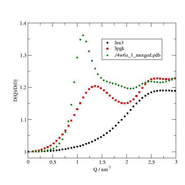
More globular proteins show a slow increase due to rotational diffusion.
For apoferritin with a hollow sphere structure we see strong peaks at length scales corresponding to the distance between the surfaces. As these are rough we see the contribution of the roughness. In between we see only translational diffusion as expected for an ideal sphere.
import jscatter as js
import numpy as np

adh = js.bio.fetch_pdb('4w6z.pdb1')
# the 2 dimers in are in model 1 and 2 and need to be merged into one.
adhmerged = js.bio.mergePDBModel(adh)

p = js.grace()
for pdb, name in zip(['3rn3','3pgk', adhmerged],
                    ['ribonuclease', 'phosphoglycerate','alcohol dehydrogenase']):
    uni = js.bio.scatteringUniverse(pdb, vdwradii={'M': 1.73,'Z':1.7},addHydrogen='pdb2pqr')
    uni.setSolvent('1d2o1')
    uni.qlist=np.r_[0.01,0.1:3:0.06]
    D_hr = js.bio.hullRad(uni)
    Dt = D_hr['Dt'] * 1e2
    Dr = D_hr['Dr'] * 1e-12
    Dq = js.bio.diffusionTRUnivTensor(uni.residues, DTT=Dt, DRR=Dr)
    p.plot(Dq.X,Dq.Y/Dq.DTTtrace, le=f'{pdb} {name}')

Dqapoferritin = js.dA(js.examples.datapath + '/apoferritin.Dq.gz')
Dqmab = js.dA(js.examples.datapath + '/mab_1igt.Dq.gz')
p.plot(Dqapoferritin.X,Dqapoferritin.Y/Dqapoferritin.DTTtrace,sy=0,li=1, le=f'1LB3 apoferritin')
p.plot(Dqmab.X,Dqmab.Y/Dqmab.DTTtrace, le=f'1igt antibody')

p.xaxis(label='Q / nm\S-1', min=0, max=3)
p.yaxis(label='D(Q)/D(0)',min=0.98,max=1.6)
p.legend(x=1.,y=1.65)
#p.save(js.examples.imagepath+'/bioeffDiffusion.jpg', size=(2, 2))
Ferritin and monoclonal antibody used above (takes longer in particular ferritin)
import jscatter as js
import numpy as np

unif = js.bio.scatteringUniverse('1LB3.pdb1')
unif.setSolvent('1d2o1')
unif.qlist=np.r_[0.1:0.5:0.1,0.5:0.7:0.01,0.7:1.2:0.02,1.2:3:0.05]
D_hr = js.bio.hullRad(unif)
Dtf = D_hr['Dt'] * 1e2
Drf = D_hr['Dr'] * 1e-12
Dqf = js.bio.diffusionTRUnivTensor(unif.residues, DTT=Dtf, DRR=Drf)
Dqf.save('apoferritin.Dq.gz')

unimab = js.bio.scatteringUniverse('1igt.pdb')
unimab.setSolvent('1d2o1')
unimab.qlist=np.r_[0.1:3:0.1]
D_hr = js.bio.hullRad(unimab)
Dtf = D_hr['Dt'] * 1e2
Drf = D_hr['Dr'] * 1e-12
Dqf = js.bio.diffusionTRUnivTensor(unimab.residues, DTT=Dtf, DRR=Drf)
Dqf.save('mab_1igt.Dq.gz')
- jscatter.bio.diffusionTRUnivYlm(objekt, Dtrans=0.0, Drot=0.0, Rhydro=0.0, **kwargs)[source]
Effective diffusion Deff of a rigid particle based on the Rayleigh expansion (Ylm).
Mixed contribution from translational and rotational diffusion in the initial slope. Only SCALAR diffusion coefficients. See [1].
- Parameters:
- objektatomgroup
Objects immersed in medium.
- qlistarray, list of float
Scattering vectors in units 1/nm.
- Dtransfloat, default = 0
Translational diffusion coefficient in nm^2/ps = 1e5 A^2/ns. If 0 calculated as \(D_{trans} = kT / (6\pi \eta R_{hydro})\) .
- Drotfloat , default = 0
Rotational diffusion coefficient in 1/ps. If 0, calculated as \(D_{rot} = kT/ (8\pi\eta R_{hydro}^3)\).
- Rhydrofloat, default = 0
Hydrodynamic radius in nm. If negative, Rhydro is calculated from the SESVolume as equivalent sphere with \(R_h=(\frac{3V_{SES}}{4\pi})^{1/3} + 0.3\) as a rough estimate.
In general the shape anisotropy needs to be accounted using
hullRad().- lmaxint; default=15
Maximum order spherical harmonics. For larger Q this needs to be increased.
- getVolume‘always’, ‘once’, ‘box’, default ‘once’
Determines volume calculation for scattering contrast.
‘always’ : For each calculation the SES/SAS volume is determined/updated using a rolling ball algorithm by
getSurfaceVolumePoints().‘once’ : Only for first call SES/SAS volume is determined using a rolling ball algorithm by
getSurfaceVolumePoints(). Some computations are speedup due to this.‘box’ : Use universe dimension to get box volume (mda.lib.mdamath.box_volume(u.dimensions)). If the box size does not change this is constant. SESVolume and SASVolume are set to the box volume.
To avoid seeing the box formfactor the solvent density in some distance of the protein/nucleic needs to be determined. See
selectSolvent().
- cubesizefloat, default None
Cube length (in units nm) for coarse graining, None means no coarse graining. For larger proteins the computation takes some time. Cubesize defines the size of a cubic grid in which atomic data as positions, formfactor and normal modes are averaged to realize a coarse graining and speedup the computation. The size should be adjusted to the protein size. This works for residue and atomic modes.
- Returns:
- dataArray [q, Deff]
Notes
According to [2] the field autocorrelation function (as measured by NSE) of a single particle \(I_1(Q,t)\) (see
intScatFuncYlm()for details) is\[I_1(Q,t) = e^{-D_{trans}Q^2t}\sum_l S_l(Q)e^{-l(l+1)D_{rot}t}\]Accordingly in the initial slope defined as \(\Gamma = Q^2D = -\lim_{t \to 0 } \bigg[\frac{d}{dt} ln(\frac{I(Q,t)}{I(Q,0)})\bigg]\) the effective diffusion Deff is [1]
\[D_{eff} = D_{trans} + \frac{\sum_l S_l(Q) l(l+1)D_{rot}}{Q^2 \sum_l S_l(Q) }\]\(S_l(Q)\) as defined in
intScatFuncYlm().References
[1] (1,2)Exploring internal protein dynamics by neutron spin echo spectroscopy R. Biehl, M. Monkenbusch and D. Richter Soft Matter, 2011, 7, 1299–1307, DOI:10.1039/c0sm00683a
[2]Effect of rotational diffusion on quasielastic light scattering from fractal colloid aggregates Lindsay H. Klein, R. Weitz, D. Lin, M. Meakin, Physical Review A 1988 vol: 38 (5) pp: 2614-2626
Examples
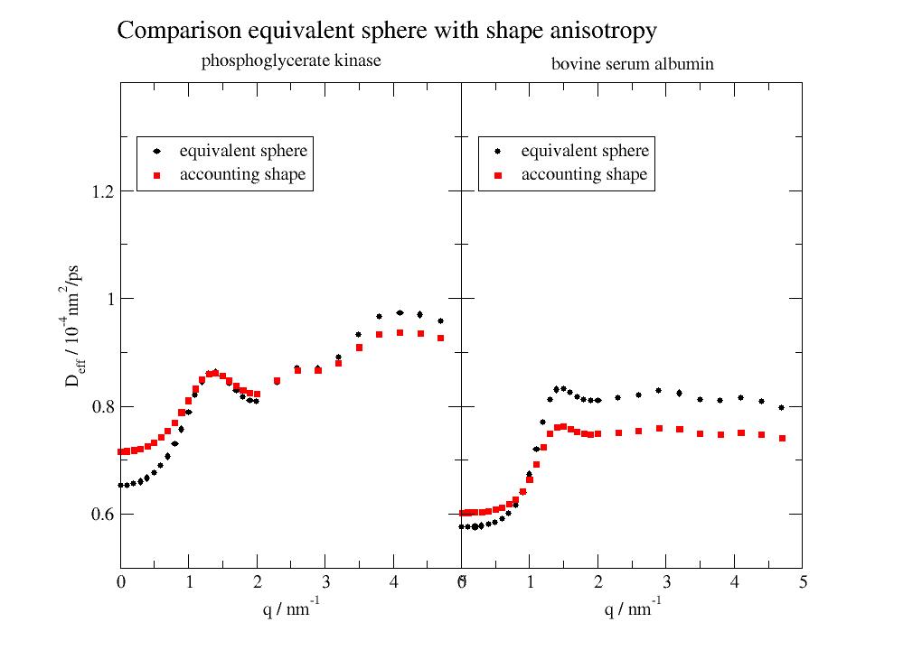
Comparison using an equivalent sphere model \(R_h=(\frac{3V_{SES}}{4\pi})^{1/3} + 0.3\) from SESVolume with an improved calculation taking the protein shape anisotropy from the pdb structure into account. Trans/rot diffusion is calculated using
hullRad().In general the shape anisotropy needs to be accounted.
import jscatter as js
import numpy as np
p=js.grace()
p.multi(1,2,hgap=0)
for i,pdb in enumerate(['3pgk', '4f5s']):
    bioassembly = js.bio.fetch_pdb(pdb, biounit=True)
    uni = js.bio.scatteringUniverse(bioassembly)
    uni.setSolvent('1d2o1')
    uni.qlist = np.r_[0.01,0.1:2:0.1,2:5:0.3]
    # Dtrans determined as sphere with SESVolume
    Dq = js.bio.diffusionTRUnivYlm(uni)
    # using hullRad which takes shape int account
    res = js.bio.hullRad(uni.select_atoms('protein'))
    # Dtrans/rot with conversion to nm²/ps and 1/ps
    Dtrans = res['Dt'] * 1e2  # nm²/ps
    Drot = res['Dr'] * 1e-12  # 1/ps
    Dq_hr = js.bio.diffusionTRUnivYlm(uni,Dtrans=Dtrans,Drot=Drot)
    p[i].plot(Dq,le='equivalent sphere')
    p[i].plot(Dq_hr, le='accounting shape ')
    p[i].xaxis(label='q / nm\S-1')
    p[i].legend(x=0.25,y=13e-5)

p[0].yaxis(min=5e-5,max=14e-5,formula='$t*1e4',label=r'D\seff\N / 10\S-4\Nnm\S2\N/ps')
p[1].yaxis(min=5e-5,max=14e-5,label='',ticklabel=False)
p.title(' '*30+'Comparison equivalent sphere with shape anisotropy',size=1.4)
p[0].subtitle('phosphoglycerate kinase')
p[1].subtitle('bovine serum albumin')
# p.save(js.examples.imagepath+'/DqYlm.jpg')
- class jscatter.bio.fakeBNM(equillibrium, k_b=418, f_d=1, vdwradii=None, cutoff=13)[source]
Bases:
brownianNMdiagFake brownian modes from explicit given configurations as displacement vectors.
Modes as displacement in direction of explicit given displaced configurations like in
brownianNMdiag.Allows also to create a subset of modes as linear combination of other modes to highlight specific motions.
- Parameters:
- equillibriumatomgroup, residues
Atomgroup or residues of universe in equillibrium positions.
If residues, Cα atoms for amino acids and for others the atom closest to the center is choosen.
- k_bfloat, default = 418.
Bonded spring constant in units g/ps²/mol.
418 g/ps²/mol = 694 pN/nm = 1(+-0.5) kcal/(molA²)as mentioned in [2]_ to reproduce a reasonable protein frequency spectrum.- f_dfloat, None
Friction of residue with surrounding residue in units g/mol/ps like in
brownianNMdiag. The friction matrix is assumed diagonal.Can be changed for fake modes using .f_d = 12.3.
- vdwradiifloat, dict, default=3.8
vdWaals radius used for neighbor bond determination like in
brownianNMdiag.- cutofffloat, default 13
Cutoff for nonbonded neighbor determination like in
brownianNMdiag.
- Returns:
- Normal Mode Analysis objectModes
Object can be indexed do get a specific Mode object representing real space displacements in unit A.
Here we have no trivial modes and indexing starts from 0 !!!.
Notes
The idea is to assume roughly that the given displacement is a “normal mode” that diagonalises the respective eigenequation with effectiveFriction and effectiveForceconstant.
The eigenvalues invRelaxTime is calculated as \(\lambda_j = k_b / \Gamma_j\) assuming that the effective force is the same for vibNM and brownianNM.
.vibNMcontains the corresponding vibrational normal mode.Examples
In the example the calcium atoms are not moving as we select only protein Cα for modes. Using a selection including calcium pins these to their neighbours as residues.
We create configurations of the Cα atoms from vibNM. The source of the modes migth be from simulation or handmade by rotating specific bonds e.g. of a linker.
import jscatter as js

uni = js.bio.scatteringUniverse('3cln_h.pdb')
org = uni.atoms.positions

# create displaced configurations
#  this an be also from simulation or different pdb structures with same number of atoms
nm = js.bio.vibNM(uni.select_atoms("protein and name CA"))

# fake residue normal modes
fake = js.bio.fakeBNM(uni.residues)
a=100
for i,j,k in [[a,a,0],[a,0,a],[0,a,a]]:
    uni.atoms.positions = org + i*nm.kTallatommode(6) + j*nm.kTallatommode(7) + k*nm.kTallatommode(8)
    fake.addDisplacement(k_b=500,f_d=1)
fake.equillibrium()

# compare the first mode to the previous ones
fake.k_b = 5
fake.f_d = 2
fake.animate([0], scale=1,kT=True).view(viewer='pymol',frames='all')
- addDisplacement(k_b=None, f_d=None)[source]
Add mode from displaced configuration from equillibrium universe.
- Parameters:
- k_bfloat
Effektive force constant of modes equivalent to
:py:class:`brownianNMdiag.effectiveForceConstant().Can be changed using .k_b = 12.3.
- f_dfloat
Friction of residue with surrounding residue/solvent in units g/mol/ps = amu/ps. Used like in
:py:class:`brownianNMdiag()as factor with number of neigbors to calculate diagonal friction matrixCan be changed using .f_d = 12.3.
Notes
Add mode v after displacement of atoms from the equillibrium positions.
v = [equillibrium - displaced]as difference vector.Creates fake normalized eigenvectors =
v_i / norm(v_i)
- property eigenvalues
Fake eigenvalues calculated from f_d and k_b on the fly
Returns list of corresponding eigenvalues for added displacements using last f_d and k_b.
\[e_i = effektiveForceConstant/effektiveFriction\]
- property k_b
- property weights
- class jscatter.bio.fakeVNM(equillibrium)[source]
Bases:
vibNMFake vibrational modes from explicit given configurations as displacement vectors.
Modes as displacement in direction of explicit given displaced configurations like in
vibNM.Allows also to create a subset of modes as linear combination of other modes to highlight specific motions.
- Parameters:
- equillibriumatomgroup, residues
Atomgroup or residues of universe in equillibrium positions.
If residues, Cα atoms for amino acids and for others the atom closest to the center is choosen.
- vdwradiifloat, dict, default=3.8
vdWaals radius used for neighbor bond determination like in
brownianNMdiag.- cutofffloat, default 13
Cutoff for nonbonded neighbor determination like in
brownianNMdiag.
- Returns:
- Normal Mode Analysis objectModes
Object can be indexed do get a specific Mode object representing real space displacements in unit A. Here we have no trivial modes and indexing starts from 0.
Notes
The idea is to assume roughly that the given displacement is a “normal mode” that diagonalises the respective eigenequation with an effectiveForceconstant.
The eigenvalue \(\omega^2\) is calculated as \(\omega^2_j = k_b / m_{eff,j}\).
Examples
In the example the calcium atoms are not moving as we select only protein Cα for modes. Using a selection including calcium pins these to their neighbours as residues.
We create configurations of the Cα atoms from vibNM. The source of the modes migth be from simulation or handmade by rotating specific bonds e.g. of a linker.
import jscatter as js

uni = js.bio.scatteringUniverse('3cln_h.pdb')
org = uni.atoms.positions

# create displaced configurations
#  this an be also from simulation or different pdb structures with same number of atoms
nm = js.bio.vibNM(uni.select_atoms("protein and name CA"))

# fake residue normal modes
fake = js.bio.fakeVNM(uni.residues)
a=100
for i,j,k in [[a,a,0],[a,0,a],[0,a,a]]:
    uni.atoms.positions = org + i*nm.kTallatommode(6) + j*nm.kTallatommode(7) + k*nm.kTallatommode(8)
    fake.addDisplacement(1)
uni.atoms.positions = org

# compare the first mode to the previous ones
fake.k_b = 500
fake.animate([0,1,2], scale=1,kT=True).view(viewer='pymol',frames='all')
- addDisplacement(k_b=None)[source]
Add mode from displaced configuration from equillibrium universe.
- Parameters:
- k_bfloat
Fake effektive force constant.
Notes
Add mode v after displacement of atoms from the equillibrium positions.
v = [equillibrium - displaced]as difference vector.Creates fake normalized eigenvectors =
v_i / norm(v_i)
- property eigenvalues
Fake eigenvalues calculated from k_b on the fly
Returns list of corresponding eigenvalues for added displacements using last f_d and k_b.
\[e_i = effektiveMass/effektiveFriction\]
- property eigenvectors
- jscatter.bio.fastpdb2pqr(input_pdb, debump=False, opt=False, drop_water=True, ph=None, whitespace=True, neutralc=False, neutraln=False, ff='PARSE', keep_chain=False, assign_only=False)[source]
A fast version of
pdb2pqr()with limited options.Default speedup is achieved by omitting optimization, debumping, minimized logging and reducing options. For full options try pdb2pqr.
- Parameters:
- input_pdbstr
Input pdb file.
- debumpbool, default False
Debump added atoms, ensure that new atoms are not rebuilt too close to existing atoms.
- optbool, default False
Perform hydrogen optimization, default is not to do it, Adjusts hydrogen positions and flips certain side chains (His, Asn, Glu) as needed to optimize hydrogen bonds.
- ff‘AMBER’,’CHARMM’,’PARSE’,’TYL06’,’PEOEPB’,’SWANSON’, default: PARSE
The forcefield to use for charge assignment.
- drop_waterbool
Drop water atoms.
- phfloat, default None
pH value to use for assignment of charges. If None pH 7 is assumed but PROPKA is not used. Cite [5] [6] if using charge assignments by PROPKA.
- neutralc, neutralnbool, default = False
Neutral C or N terminal.
- keep_chainbool, default: False
Keep the chain ID in the output PQR file
- assign-onlybool, default: False
Only assign charges and radii - do not add atoms, debump, or optimize.
- whitespacebool
Insert whitespaces between atom name and residue name, between x and y, and between y and z. This improves readability but breaks PDB file definition.
- Returns:
- input_pdb_h.pqr, input_pdb_h.pdb (without previous suffix)
Notes
- Uses default fast options of pdb2pqr except of these.
debump = False
opt = False
drop_water = True ; this reduces just the number of atoms not to get errors in mda
whitespace; mda has problems as somewhere split() is used instead of char numbers as defined for pqr files
pdb_output = input_pdb with prefix appended ‘_h’
References
[3]Improvements to the APBS biomolecular solvation software suite. Jurrus E, et al. Protein Sci 27 112-128 (2018).
[4]PDB2PQR: expanding and upgrading automated preparation of biomolecular structures for molecular simulations. Dolinsky TJ, et al. Nucleic Acids Res 35 W522-W525 (2007).
[5]Improved Treatment of Ligands and Coupling Effects in Empirical Calculation and Rationalization of pKa Values Sondergaard, Chresten R., Mats HM Olsson, Michal Rostkowski, and Jan H. Jensen. Journal of Chemical Theory and Computation 7, (2011): 2284-2295.
[6]PROPKA3: consistent treatment of internal and surface residues in empirical pKa predictions. Olsson, Mats HM, Chresten R. Sondergaard, Michal Rostkowski, and Jan H. Jensen. Journal of Chemical Theory and Computation 7, no. 2 (2011): 525-537.
Examples
Meanwhile Jscatter >1.8.3 the charges are always added. Use fastpdb2pqr and combine the ‘_h.pdb’ file including ligands but without charges with the ‘_h.pqr file’ that contains charges but no ligands.
To get charge states of ligands please use the web services or programs mentioned in
pdb2pqr().Charges can be added manually for the ligands.
import jscatter as js
import MDAnalysis as mda

# this adds hydrogen to uni with ligands  and adds charges in the corresponding '.pqr' file
uligand = js.bio.scatteringUniverse('3pgk')
uligand.add_TopologyAttr('charges')  # all charges are zero
ucharge = js.bio.scatteringUniverse('3pgk_h.pqr')
protein = ucharge.select_atoms('protein').atoms
for l,c in zip(uligand.select_atoms('protein').residues, ucharge.select_atoms('protein').residues):
    try:
        # this throws an error if len(charges) is different; in that way same residues get correct charge
        l.atoms.charges =c.atoms.charges
    except:
        print('---',l.resnum,c.resnum)

uligand.atoms.charges.sum()  # = -1
- jscatter.bio.fetch_pdb(id, path='./', biounit=False, timeout=5)[source]
Fetch id from pdb databank at http://www.rcsb.org/
- idstring
PDB id 4 letter code of protein structure
- pathstring
path where to store the file
- biounitbool, int
Download biounit/assembly1 with ending .pdb[biounit] as e.g. .pdb1.
- timeoutfloat
Timeout for the donwload.
- Returns:
- Saves gunziped file and returns corresponding path.
Notes
Biounit/assembly can be downloaded using file ending .pdb1 or .pdb2
- jscatter.bio.getDistanceMatrix(objekt, cutoff=None)[source]
Distance matrix for atoms in objekt.
objekt migth be a selection to get e.g. distances between CA or H atoms
- Parameters:
- objektAtomGroup or residueGroup
Objekt to get distance matrix.
- cutofffloat
Cutoff radius. For larger distances 0 is returned.
- Returns:
- Distance matrix NxN (upper triagonal) in units nm.
Notes
For larger matrices a faster neighbor search is used.
Examples
import jscatter as js

uni=js.bio.scatteringUniverse('3pgk')
u = uni.select_atoms("protein and type H")
dd = js.bio.getDistanceMatrix(u)

u = uni.select_atoms("protein and name CA")
dd = js.bio.getDistanceMatrix(u,cutoff=2)
- jscatter.bio.getNativeContacts(objekt, overlap=0.01, vdwradii=None)[source]
Creates a native contact residue dict for a given object for Go-like protein modeling.
- A residue j is added as contact to residue i if any atom van der Waals radii overlap
\(R_i^{vdW} + R_j^{wdW}-overlap < distance(i,j)\)
- objekt :
group of atoms
- overlap :
Overlap of van der Waals radii to be counted as in contact in units nm.
- vdwradiidictionary
Van der Waals radii to use in units nm.
- Returns:
- dict with {residuelist of residue in contact }
- or
list of index pairs for bonds
References
[1]Prediction of hydrodynamic and other solution properties of partially disordered proteins with a simple, coarse-grained model. Amorós, D., Ortega, A., & De La Torre, J. G. (2013). Journal of Chemical Theory and Computation, 9(3), 1678–1685. https://doi.org/10.1021/ct300948u
[2]Selection of Optimal Variants of Gō-Like Models of Proteins through Studies of Stretching Joanna I. Sułkowska Marek Cieplak Biophysical Journal 95,3174-3191 (2008) https://doi.org/10.1529/biophysj.107.127233
Examples
import jscatter as js
from collections import defaultdict

# all atom universe with hydrogen
uni=js.bio.scatteringUniverse('3pgk')
u = uni.select_atoms("protein")
NN1 = js.bio.getNativeContacts(u)

# CA atom group
u = uni.select_atoms("protein and name CA")
# use a larger van der Waals radius for CA only with 3.8A as distance between CA along backbone
NN2 = js.bio.getNativeContacts(u, vdwradii=defaultdict(lambda: 3.8, {'C':3.8}))
- jscatter.bio.getOccupiedVolume(atoms, dl=0.12)[source]
Calculates Voronoi cell volume for atom positions in a filled universe box. Only for filled boxes meaningful.
A universe box gets 26 copies of itself around the central original box (periodic boundary conditions in MD). From these the layer with thickness dl around the center universe box is used to get neigbors for the close to box boundary positions. This guarranties proper neigbors, a filled box and \(\sum V_{atoms} = box volume\).
- Parameters:
- atomsuniverse atoms or residues
Atom positions are used for Voronoi cell volume.
- dlfloat
Border size to include in convexHull as fraction from box size.
- Returns:
- arrayfloats
Voronoi cell volumes in units A³ for the atoms.
Notes
scipy.spatial.Voronoi and scipy.spatial.convexHullVolume are used to calc the volume per atom.
- jscatter.bio.getSurfaceVolumePoints(objekt, point_density=5, probe_radius=0.13, surfacename='1', vdwradii=None, shellthickness=0.3)[source]
Calculates the solvent excluded volume (SES and SAS) for a dense object like protein or DNA.
It is NOT necessary to call this function as it is called automatically from all scattering functions and determines the surface atoms and the objekt volume. It is less accurate for solvent boxes as these may have space in between molecules and need adjusted probe_radius.
- Parameters:
- objektatom group
Atom group.
- point_densityinteger, default 5
Point density on surface of each atom for rolling ball algorithm as n_points = 2**(2*point_density)+2 On error it is automatically incremented
- probe_radiusfloat, default 0.13 nm for water
Probe radius for SAS/SES calculation.
- shellthicknessfloat
Shell thickness of the surface layer. The default is 0.3.
- surfacenamestr
Name for surface selection
- vdwradiidict, default None
Dictionary of van der Waals radii for rolling ball algorithm in units nm.
If None the vdW radii used in the object universe are used. See notes below.
I a defaultdict only these values are used. This is used e.g. for Calpha or coarse grain models to use only the given defaults like vdwradii = defaultdict(lambda :0.38) .
- Returns:
- None
Universe topology attributes surface and surfdata are populated
per surface atom with .surfdata = [surface area, SASvolume, shellVolume, surfmean position]
adds to objekt.universe .SASVolume volume SAS
adds to objekt.universe .SESVolume volume SES
adds to objekt.universe .SASArea
surface area can be calculated universe.select_atoms(‘surface 1’).surfdata[:,0].sum()
SASVolume is universe.select_atoms(‘surface 1’).surfdata[:,1].sum()
dummy bead positions in surface layer universe.select_atoms(‘surface 1’).surfdata[:,3:]
Notes
SES/SAS see Accessible surface area
SAS area/volume (solvent-accessible surface) is the surface area of a molecule that is accessible to a solvent center. SAS area is calculated by sasa.aVSPointsGradients.
SAS area is here calculated using the rolling ball algorithm developed by Shrake & Rupley [1]. It describes the surface of the center of a probe molecule (ball) with probe_radius rolling over the van der Waals surface. We use a probe_radius of 0.13 nm that represents the radius of a water molecule.
SES area/volume (solvent excluded surface) is defined by the envelope excluding the volume occupied by the rolling ball probe. Also called Connolly surface [5] .
Method assuming a object like a protein (not solvent like water)
Shrake/Rupley rolling ball algorithm:
For each atom a regular angular grid of \(N_{SAS}\) points builds a surface S in a distance \(d=R_{vdW} +R_{probe}\) of the atomic vdWaals surface. \(R_{probe}\) represents the solvent size. The points in S are tested for overlap with the same surface of other neighboring atoms. The set of non overlapping points build the SAS surface enclosing the SAS volume of the atom group. The SAS points have a distance \(R_{probe}\) from the van der Waals surface of the atoms.
The SESVolume as a kind of dry volume is \(V_{SES} = V_{SAS} - V_{surface layer}\). The surface layer volume \(V_{surface layer}\) for each atom i may be estimated as the volume between previous determined SAS points p and the van der Waals surface with volume per SAS point \(V_{p,i} = 4/3\pi ((R_{vdW,i}+R_{probe})^3 - R_{vdW,i}^3) / N_{SAS}\).
In each corner (touching atoms) the probe surface sphere describes a smooth surface not reaching into the corner. This missing volume can be approximated using the rolling ball algorithm with same number of points \(N_{SAS}\) but reduced probe radius \(R_{probe}/2\). Each additional appearing point not in the original SAS surface contributes a volume \(V_{p,c} = 4/3\pi (R_{probe})^3 / N_{SAS}\) as sector from the probe center located in the SAS corner. Also buried atoms (between non-touching atoms which are not in the SAS surface) contribute with the same amount. It should be mentioned that this is an approximation for the corner probe sphere volume as the points distributed around the original atoms show a small deviation compared to atoms distributed around probe spheres located in the corner. On the other hand most algorithms describe only an approximation.
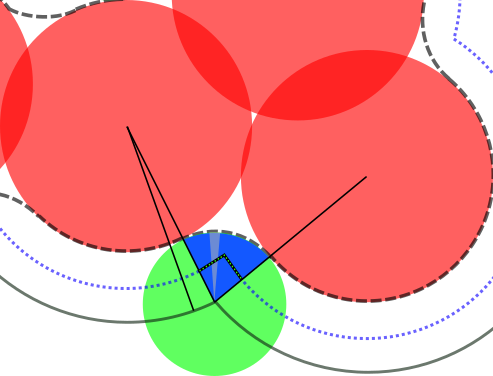
red: atoms, green: probe, solid line: SAS, dashed: SES, dots: probe R/2 points, blue: additional layer volume corner with additional points and probe section per point
A comparison to experimental determined protein densities is shown in Protein density determination. For a probe radius of 1.3 A, we find excellent agreement. 1.3 A corresponds to the reduced oxygen vdW radius for proper protein density determination.
As vdWaals radii we use for the atoms H, C, N, O the observed radii according to Fraser at al [2]. For H this corresponds to 1.07 A which is a bit smaller comapred to the revised value 1.1 of Rowland et al. [3]. For other values we use vdWaals radii of Bondi et al. [4] which are rare for proteins.
For the determination of the hydration layer contributing to the neutron/X-ray scattering usually a 0.3 nm hydration layer is assumed as e.g. in CRYSON/CRYSOL. To determine the respective hydration layer volume we use the same approach as above with the shellthickness parameter. By default, we use a thickness of 0.3 nm for the hydration layer if no other value is given.
It should be noted that compared to CRYSOL the scattering pattern is a bit different at larger Q. CRYSOL fits the parameter r0 as an adjustment to the listed vdW radius mainly changing the excluded volume scattering. The values of CYSOL can be repdoduced by seting the H vdW radius to 1.2 A
universe.select_atoms('name H').vdWradiinm =.12which result in a different protein density.References
[1]Environment and exposure to solvent of protein atoms. Lysozyme and insulin Shrake, A; Rupley, JA. (1973). J Mol Biol. 79 (2): 351–71. doi:10.1016/0022-2836(73)90011-9.
[2]An improved method for calculating the contribution of solvent to the X-ray diffraction pattern of biological molecules. Fraser, R. D. B., MacRae, T. P., & Suzuki, E. (1978). Journal of Applied Crystallography, 11(6), 693–694. https://doi.org/10.1107/S0021889878014296
[3]Intermolecular Nonbonded Contact Distances in Organic Crystal Structures: Comparison with Distances Expected from van der Waals Radii. R. Scott Rowland, Robin Taylor The Journal of Physical Chemistry. Bd. 100, Nr. 18, 1996, S. 7384–7391, doi:10.1021/jp953141
[4]van der Waals Volumes and Radii. A. Bondi The Journal of Physical Chemistry. Bd. 68, Nr. 3, 1964, S. 441–451, doi:10.1021/j100785a001
[5]Analytical molecular surface calculation Connolly, M. L. J. Appl. Crystallogr. 16, 548–558 (1983). doi:10.1107/S0021889883010985.
- jscatter.bio.intScatFuncOU(brownianmodes, nm, **kwargs)[source]
ISF I(q,t) for Ornstein-Uhlenbeck process of normal mode domain motions in a harmonic potential with friction.
Displacements along normal modes in harmonic potential with additional internal friction leading to overdamped motions along Brownian Modes. The theory is described in [1] and [2] and applied to an immunoglobulin in [3].
The model relates internal friction and force constants to amplitudes and relaxation times
- Parameters:
- brownianmodesbrownianMode object
Brownian normal modes => the force constant matrix normalized to friction
brownianNMdiag()andfakeBNM()contain below frictional displacements \(e_{jk}\) and corresponding vibrational displacements \(d_{jk}\).Friction and forceconstants are defined in mode object and change \(e_{jk}\) and \(d_{jk}\).
- nmlist of int
Indices of the modes starting with 6 for first nontrivial mode.
- getVolume‘always’, ‘once’, ‘box’, default ‘once’
- Determines volume calculation for scattering contrast.
‘always’ : For each calculation the SES/SAS volume is determined/updated using a rolling ball algorithm by
getSurfaceVolumePoints().‘once’ : Only for first call SES/SAS volume is determined using a rolling ball algorithm by
getSurfaceVolumePoints(). Some computations are speedup due to this.‘box’ : Use universe dimension to get box volume (mda.lib.mdamath.box_volume(u.dimensions)). If the box size does not change this is constant. SESVolume and SASVolume are set to the box volume.
To avoid seeing the box formfactor the solvent density in some distance of the protein/nucleic needs to be determined. See
selectSolvent().
- cubesizefloat, default None
Cube length (in units nm) for coarse graining, None means no coarse graining. For larger proteins the computation takes some time. Cubesize defines the size of a cubic grid in which atomic data as positions, formfactor and normal modes are averaged to realize a coarse graining and speedup the computation. The size should be adjusted to the protein size. This works for residue and atomic modes.
- used from modes or universe:
invRelaxTimes = \(\lambda_j\) in units 1/ps.
u.tlist : time points from universe in units ps.
u.qlist : scattering vector q from universe in units 1/nm.
u.temperature : u.temperature from universe in units K.
scattering mode as ‘n’ or ‘x’ is allowed. For neutron scattering the result corresponds to NSE while for ‘x’ the results corresponds to X-ray photon correlation spectroscopy (XPCS).
- Returns:
- dataListlist of dataArray
.X : time points
.Y : Fqt(t)/Fqt(t=0) coherent, equ 11+41+49+79 with 81 in [1]
.q scattering vector unit 1/nm
.relaxationtimes
.effectiveFriction effectiveFriction of modes see NMmode
.effectiveForceConstant effectiveForceConstants of modes
.Sqt0 amplitude for t=0 equ 11+41+79 with 81 in [1]
.Sqtinf_DW amplitude t=inf , equ 11+41+49 in [1] Debye-Waller like factor in [1]
.Sqt00 amplitude t=0 , equ 11+41+50 in [1] in [1]
.Sq_amp0 sum_i_j[bi*bj] = no displacements = normal formfactor without DW
.elasticplateau Sqtinf_DW[0]/Sqt0 ; (1-elasticplateau) is the NSE amplitude
.frictionPerMode friction mode weighted by mode vectors = b*frict*b
.brownianModeRMSD mode RMSD
Notes
The dynamics of a protein can be described under the assumption of dynamic decoupling [3] by a combination
\[F(Q,t) = F_{trans}(Q,t) \cdot F_{rot}(Q,t) \cdot F_{int}(Q,t)\]The intermediate scattering function \(F_{int}(Q,t)\) of atoms or subunits k with scattering length \(b_k\) at positions \(R_k\) describing our internal dynamics can be written as
\[F(Q,t) = \Big \langle \sum_{k,l} b_kb_l e^{iQR_k(t)}e^{iQR_l(0)} \Big \rangle\]With displacements \(u_k\) from equilibrium position \(R_k^{eq}\) we can use \(R_k=R_k^{eq} + u_k(t)\) resulting in
\[F(Q,t) = \Big \langle \sum_{k,l} b_kb_l e^{iqR_k^{eq}}e^{iqR_l^{eq}} f_{kl}(Q,\infty) f_{kl}^{\prime}(Q,t) \Big \rangle\]The constant term is related to the 3N vibrational modes j and only dependent on the harmonic potential as
\[f_{kl}(Q,\infty) = exp \Big(-\sum_{j=1..3N} \frac{1}{2} ((d_{jk}\cdot Q)^2 + (d_{jl} \cdot Q)^2) \Big)\]with vibrational displacements \(d_{jk} = \sqrt{kT/(m_k\omega_j^2)}\hat{v}_{jk}\) for elastic normal mode \(\hat{v}_j\) that correspond to the width in a Gaussian distribution around the equilibrium configuration in a potential with mean force constant \(k_j=m_j^{eff}\omega_j^2\) (effective mass \(m_j^{eff}\)). See
vibNM()for elastic modes. With increasing \(\omega\) the mode amplitudes become smaller.In the high friction limit the time dependent part within Smoluchowski dynamics (friction dominated) is described by
\[f_{kl}^{\prime}(Q,0) = exp \Big(\sum_{j=1..3N} (e_{jk}Q)(e_{jl}Q)e^{-\lambda_jt} \Big)\]with displacements \(e_{jk} = \sqrt{kT/(\lambda_j\Gamma_j)}\hat{b}_{jk}\) for Brownian mode \(\hat{b}_j\), mode friction \(\Gamma_j = \hat{b}^T\gamma\hat{b}\) and inverse mode relaxation time \(\lambda_j\). The displacement \(e_{jk}\) corresponds to the displacement within relaxation time \(1/\lambda_j\). See
brownianNMdiag()for Brownian modes and the definition of the friction matrix \(\gamma\) that defines the mode with the force constant matrix.
While the vibrationel modes with
k_bdetermine the width of the configurational room around the equillibrium the brownian modes decribe in which direction the relaxation movement evolve.Taylor expansion of the Smoluchowsky dynamics leads to a description for small displacements (or low Q) [1] that results in a description as found in
intScatFuncPMode()Friction related to translational diffusion can be estimated from \(f=kT/D\).
Equipartition determine force constant from msd \(f<x^2>/2 = 0.5kT ==> f= kT/<x^2>\)
dummy surface atoms are ignored.
References
[1] (1,2,3,4,5,6)Inelastic neutron scattering from damped collective vibrations of macromolecules Gerald R. Kneller Chemical Physics 261, 1-24, (2000)
[2]Harmonicity in slow protein dynamics Hinsen K. et al. Chemical Physics 261, 25, (2000)
Examples
The small protein calmodulin as example. Domain motions might be quite fast as here for demonstration the internal friction is choosen low. This is a synthetic example without experimental proof just as demonstration. See [3] for experimental result using antibodies.
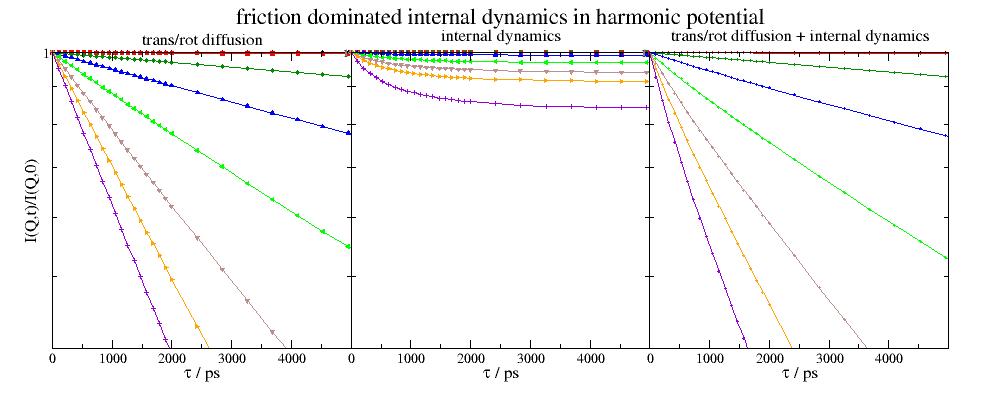
import jscatter as js
import numpy as np
uni=js.bio.scatteringUniverse('3CLN')
uni.qlist=np.r_[0.01,0.1:2:0.3]
uni.tlist = np.r_[1:2000:20j,2000:10000:20j]
uni.setSolvent('1d2o1')

# rigid protein trans/rot diffusion
hR = js.bio.hullRad(uni.atoms)
Dtrans = hR['Dt'] * 1e2  # in nm²/ps
Drot = hR['Dr'] * 1e-12  # in 1/ps
Iqt = js.bio.intScatFuncYlm(uni.residues, Dtrans=Dtrans, Drot=Drot)

# internal domain motions
bnm = js.bio.brownianNMdiag(uni.residues,k_b=70, f_d=5)
OU = js.bio.intScatFuncOU(bnm, [6,7,8])

# combine diffusion and internal dynamics
IqtOU = Iqt.copy()
for i, iqtou in enumerate(IqtOU):
   ou = OU.filter(q=iqtou.q)[0]
   # combining in this case its just multiplication in time domain
   iqtou.Y = iqtou.Y * ou.Y

# show the result comparing the contributions
p=js.grace(2,0.8)
p.multi(1, 3, hgap=0)
p[0].plot(Iqt,li=-1)
p[1].plot(OU,li=-1)
p[2].plot(IqtOU,sy=[1,0.3,-1],li=-1)
for i in [0,1,2]:
   p[i].xaxis(label=r'\xt\f{} / ps',min=0,max=4999,charsize=1.5)
   p[i].yaxis(scale='log',min=0.4,max=1)
p[0].yaxis(label='I(Q,t)/I(Q,0)',charsize=1.5)
p[0].subtitle('trans/rot diffusion',size=1.5)
p[1].subtitle('internal dynamics',size=1.5)
p[2].subtitle('trans/rot diffusion + internal dynamics',size=1.5)
p[1].title('friction dominated internal dynamics in harmonic potential',size=2)
#p.save(js.examples.imagepath+'/iqtOrnsteinUhlenbeck.jpg',size=(1000,400))
- jscatter.bio.intScatFuncPMode(modes, n, **kwargs)[source]
Dynamic mode form factor P_n(q) to calculate ISF of normal mode displacements in small displacement approximation.
Mode n contribution to ISF \(I(Q,t)/I(Q,0) = e^{-\lambda t}\hat{P}(Q)\) or additional contribution to the diffusion coefficient in initial slope \(\Delta D_{eff}(Q)\) .
- Parameters:
- modesnormal mode objekt
Normal modes.
- nint
Index of normal mode.
- getVolume‘always’, ‘once’, ‘box’, default ‘once’
Determines volume calculation for scattering contrast.
‘always’ : For each calculation the SES/SAS volume is determined/updated using a rolling ball algorithm by
getSurfaceVolumePoints().‘once’ : Only for first call SES/SAS volume is determined using a rolling ball algorithm by
getSurfaceVolumePoints(). Some computations are speedup due to this.‘box’ : Use universe dimension to get box volume (mda.lib.mdamath.box_volume(u.dimensions)). If the box size does not change this is constant. SESVolume and SASVolume are set to the box volume.
To avoid seeing the box formfactor the solvent density in some distance of the protein/nucleic needs to be determined. See
selectSolvent().
- cubesizefloat, default None
Cube length (in units nm) for coarse graining, None means no coarse graining. For larger proteins the computation takes some time. Cubesize defines the size of a cubic grid in which atomic data as positions, formfactor and normal modes are averaged to realize a coarse graining and speedup the computation. The size should be adjusted to the protein size. This works for residue and atomic modes but needs enough atoms in a cube.
- used from modes or universe:
modes.u.qlist : scattering vector q from mode universe in units 1/nm
modes.u.temperature : temperature of the mode universe
scattering mode as ‘n’ or ‘x’ is allowed. For neutron scattering the result corresponds to NSE while for ‘x’ the results corresponds to X-ray photon correlation spectroscopy (XPCS).
displacements from kTdisplacements are used. See the corresponding mode type.
- Returns:
- dataArray[q, Pn, Fq, Pninc]
q scattering vector, units 1/nm
Pn coherent dynamic formfactor of mode \(\alpha\), unit nm²
Pninc incoherent dynamic formfactor of mode \(\alpha\), unit nm²
Fq coherent formfactor, unit nm²
Pn and Pninc relate to mode(i).kTdisplacement = \(\vec{d}_{\alpha}=\sqrt{\frac{kT}{k_{\alpha}}}\hat{v}\) in thermal equilibrium. A scalar scaling factor scales accordingly the force constants used for normal mode calculation.
Notes
The formfactor is
\[F(Q) = \Big \langle \sum_{k,l} b_kb_l e^{iQ(r_k-r_l)} \Big \rangle\]for atoms k,l with respective scattering length b.
Assuming that fluctuations around the equillibrium configuration are dominated by friction instead of elastic forces we expect exponential relaxation of displacements. (see
brownianNMdiag())For small displacements \(d\) along normal mode a, F(Q,t) may be obtained in analogy to a 1-phonon approximation of the cross section as [1] (for incoherent k=l and \(b_k=b_{k,inc}\)):
\[F(Q,t) = F(Q) + \sum_{\alpha} e^{-\lambda_{\alpha} t} P_{\alpha}(Q)\]with
\[P_{\alpha}(Q) = \Big \langle \sum_{k,l} b_kb_l e^{iQ(r_k-r_l)} (\vec{Q}*\vec{d}_{\alpha,k}) (\vec{Q}*\vec{d}_{\alpha,l}) \Big \rangle\]and normal mode displacements \(\vec{d}_{\alpha,l} = a_{l,\alpha} \hat{v}_{\alpha,l}\) of weighted orthogonal eigenvectors \(\hat{v}_{\alpha,l}\).
For elastic modes in thermal equilibrium the mode amplitude \(a\) is related to the (effective) elastic mode force constant \(k_{\alpha}=m\omega^2_{\alpha}\) (and eigenfrequency) by \(a_{l,\alpha} =\sqrt{\frac{kT}{k_{\alpha}}} = \sqrt{\frac{kT}{m_l\omega^2_{\alpha}}}\)
We yield for the ISF of multiple modes [2]:
\[\begin{split}I(Q,t)/I(Q,0) &= \frac{F(Q) + \sum_{\alpha} e^{-\lambda_{\alpha} t} P_{\alpha}(Q)}{[F(Q) + \sum_{\alpha} P_{\alpha}(Q)]} \\ &= (1-A(Q)) + A(Q) e^{-\lambda t}\end{split}\]with with commmon relaxation rate \(\lambda\) and \(A(Q) = \frac{\sum_{\alpha} P_{\alpha}(Q)}{[F(Q) + \sum_{\alpha} P_{\alpha}(Q)]}\) . Note that \(P_{\alpha}\) are summed and not averaged for multiple modes.
We use here .kTdisplacements \(\vec{d}_{\alpha,l} = a_{l,\alpha} \hat{v}_{\alpha,l}\) of given normal modes that the amplitudes correspond to displacements in thermal equillibrium and modes are weighted by the eigenvalues.
A common relaxation time or use independent relaxation times can be used. It should be mentioned that the eigenvalues depend on geometry and atomic force constants and therefore are to some extent vague.
The additional contribution to the effective diffusion coefficient of a single mode in initial slope is [1]:
\[\Delta D_{eff}(Q) = \frac{\lambda_{\alpha} a_{\alpha}^2 P_{\alpha}(Q)}{Q^2[F(Q)+a_{\alpha}^2 P_{\alpha}(Q)]}\]with the inverse relaxation time \(\lambda_{\alpha}\) and a mode amplitude scaling factor \(a_{\alpha}\). The amplitude scaling factor can be used for fitting
dummy surface atoms are ignored.
References
[1] (1,2,3,4)Direct Observation of Correlated Interdomain Motion in Alcohol Dehydrogenase Biehl R et al.Phys. Rev. Lett. 101, 138102 (2008)
[2]Large Domain Fluctuations on 50-ns Timescale Enable Catalytic Activity in Phosphoglycerate Kinase R. Inoue, R. Biehl, T. Rosenkranz, J. Fitter, M. Monkenbusch, A. Radulescu, B. Farago, and D. Richter Biophysical Journal 99, 2309–2317 (2010), doi: 10.1016/j.bpj.2010.08.017
Examples
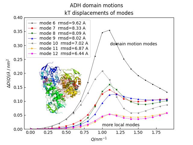
Alcohol dehydrogenase is a tetramer with 4 clefts where the active center is located.
The PDB structure presents a structure with 2 clefts in a closed configuration with bound cofactor NADH and in 2 clefts an open configuration without cofactor.
The following normal mode analysis identifies modes with large domain movements similar to [1]. In [1] a configuration of 4 open clefts and 4 closed clefts is compared.
%matplotlib
import jscatter as js
import numpy as np
import matplotlib.image as mpimg

adh = js.bio.fetch_pdb('4w6z.pdb1')
# the 2 dimers in are in model 1 and 2 and need to be merged into one.
adhmerged = js.bio.mergePDBModel(adh)
uni=js.bio.scatteringUniverse(adhmerged)
uni.qlist=np.r_[0.01,0.1:2:0.1]
uni.setSolvent(['1D2O1','0H2O1'])  # includes density 1.105 g/cm³

# do normal mode analysis without cofactors but 2 clefts still closed
nm = js.bio.vibNM(uni.select_atoms('protein').residues)

p = js.mplot()
a=150
for NN in [6,7,8,9,10,11,12]:
   Ph = js.bio.intScatFuncPMode(nm, NN)
   p.Plot(Ph.X, a**2 * Ph._Pn / (Ph._Fq+a**2*Ph._Pn) / Ph.X**2, le=f'mode {NN}  rmsd={Ph.kTrmsd*a:.2f} A')

p.Yaxis(label=r'$\Delta D(Q)/\lambda \;/\; nm^2 $',min=0,max=0.4)
p[0].Xaxis(label=r'$Q / nm^{-1}$')
p[0].Legend()
p.Text(string='domain motion modes',x=1.11,y=0.3)
p.Text(string='more local modes',x=1,y=0.01)
p.Title('ADH domain motions')
p[0].set_title('kT displacements of modes')

# add image
adhimg = mpimg.imread(js.examples.imagepath+'/adh.png')
axin = p[0].inset_axes([0.,0.05,0.5,0.6])
axin.imshow(adhimg)
axin.axis('off')
# p.Save(js.examples.imagepath+'/biodeltaDeff.jpg')
- jscatter.bio.intScatFuncYlm(objekt, Dtrans=0.0, Drot=0.0, Rhydro=0.0, **kwargs)[source]
ISF based on the Rayleigh expansion for diffusing rigid particles with scalar Dtrans/Drot .
I(q,t)/I(q,0) based on the Rayleigh expansion for scalar translational and rotational diffusion as described in [2] and used in [1] .
- Parameters:
- objektuniverse
Atomgroup universe
- tlistarray, default = 10 values between 100ps to 100ns
Time points in ps units. If None it is taken from objekt.universe.tlist.
- qlistarray, list of float
Scattering vectors in units 1/nm.
- Dtransfloat, default = 0
Translational diffusion coefficient in nm^2/ps = 1e5 A^2/ns. If 0 calculated from Rhydro.
- Drotfloat , default = 0
Rotational diffusion coefficient in 1/ps If 0 calculated from Rhydro
- Rhydrofloat, default = 0
Hydrodynamic radius in nm. If negative, Rhydro is calculated from the SESVolume as equivalent sphere with \(R_h=(\frac{3V_{SES}}{4\pi})^{1/3} + 0.3\) as a rough estimate.
In general the shape anisotropy needs to be accounted using
hullRad().- lmaxint; default=15
Maximum order spherical harmonics.For larger Q this needs to be increased.
- kwargs
Additional keyword arguments are passed to diffusionTRUnivYlm
- getVolume‘always’, ‘once’, ‘box’, default ‘once’
Determines volume calculation for scattering contrast.
‘always’ : For each calculation the SES/SAS volume is determined/updated using a rolling ball algorithm by
getSurfaceVolumePoints().‘once’ : Only for first call SES/SAS volume is determined using a rolling ball algorithm by
getSurfaceVolumePoints(). Some computations are speedup due to this.‘box’ : Use universe dimension to get box volume (mda.lib.mdamath.box_volume(u.dimensions)). If the box size does not change this is constant. SESVolume and SASVolume are set to the box volume.
To avoid seeing the box formfactor the solvent density in some distance of the protein/nucleic needs to be determined. See
selectSolvent().
- cubesizefloat, default None
Cube length (in units nm) for coarse graining, None means no coarse graining. For larger proteins the computation takes some time. Cubesize defines the size of a cubic grid in which atomic data as positions, formfactor and normal modes are averaged to realize a coarse graining and speedup the computation. The size should be adjusted to the protein size. This works for residue and atomic modes.
- Returns:
- dataList with a dataArray for each q in qlist
to get only I(q,t) as Y values use cohIntScaIntUnivYlm(….)[0].Y
Notes
We use equ 24 in [2] to calculate the field autocorrelation function of a single particle \(I_1(Q,t)\)
\[I_1(Q,t) = e^{-D_{trans}Q^2t}\sum_l S_l(Q)e^{-l(l+1)D_{rot}t}\]where NSE measures \(I_1(Q,t)/I_1(Q,t=0)\) as described in [1].
The partial scattering amplitudes \(S_l(Q)\) are defined as
\[S_l(Q) = \sum_m \bigg| \sum_j b_j(Q)j_l(Qr_j) Y_{lm}(\Omega_j) \bigg|^2\]where \(j_l\) are the spherical Bessel functions, \(Y_{lm}\) are spherical harmonics and \(\Omega_{j}\) denotes the orientation of the position vector of the atom at position \(r_j\) with scattering amplitude \(b_j\).
For larger Q a larger lmax is needed as it defines the resolution of the calculation.
References
Examples
import jscatter as js
import numpy as np
uni = js.bio.scatteringUniverse('3pgk')
uni.qlist = np.r_[0.01,0.1:2:0.2]
uni.tlist = np.r_[1,10:1e4:50]
uni.setSolvent('1d2o1')
# Without arguments Dtrans/Drot correspond to sphere volume of SESVolume
Iqt = js.bio.intScatFuncYlm(uni.residues)
p = js.grace()
p.plot(Iqt)
p.yaxis(label=r'I(Q,t)/I(Q,0)')
p.xaxis(label=r'\xt\f{} / ps')
p.title('ISF for translational/rotational diffusion')
#p.save(js.examples.imagepath+'/iqttranrot.jpg')
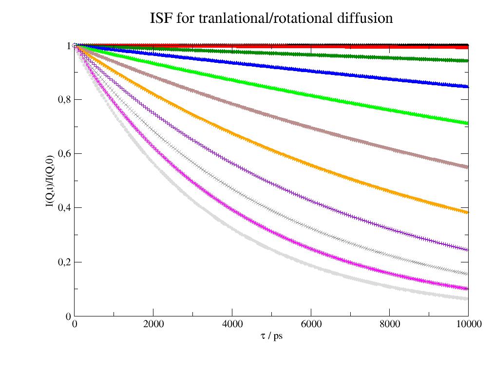
- jscatter.bio.mergePDBModel(pdb)[source]
Merge models in PDB structure from biological assembly to single model.
Biological units are saved as multi model PDB files. mergePDBmodel merges these multiple models into one model that can be read by MDAnalysis or other programs as multimeric protein.
- Parameters:
- pdbstring,filename
PDB id or filename with models to merge.
- Returns:
- merged filename
Examples
Fetch ferritin (24-mer) 1lb3 biological assembly and merge to one frame. The example needs some time
import jscatter as js
fer = js.bio.fetch_pdb('1lb3',biounit=True)
merged_filename = js.bio.mergePDBModel(fer)

# to show it
uni = js.bio.scatteringUniverse(merged_filename, addHydrogen=False)
uni.view(viewer='pymol')
- jscatter.bio.nscatIntUniv(objekt, qlist=None, **kwargs)[source]
Neutron scattering intensity with contrast to solvent.
See
scatIntUniv()with mode=’n’ for details.
- jscatter.bio.pdb2pqr(input_pdb, output, *args, **kwargs)[source]
Adds hydrogen to pdb structures, optional determines charges and repairs missing atoms.
Interface to pdb2pqr in interactive shell. Original source is at [1], [2], Please cite [3],[Re08193610e87-4]_. From original documentation at [2] :
Adding a limited number of missing heavy (non-hydrogen) atoms to biomolecular structures. Estimating titration states and protonating biomolecules in a manner consistent with favorable hydrogen bonding. Assigning charge and radius parameters from a variety of force fields. Generating “PQR” output compatible with several popular computational modeling and analysis packages.
Not all options work currently as the used CLI interface takes special format options. For most cases
fastpdb2pqr()works fine.- Parameters:
- input_pdbstring
Path to input pdb file. If only the pdb ID the corresponding file is downloaded.
- outputstring
Path of output file.
- argsstrings
Positional arguments are prepended by –xxx to represent options without input parameter
If ‘-’ is in key exchange it by underscore ‘_’.
- kwargspairs key=value
Keyword arguments for options with input value. passed as ‘–key value ‘
If ‘-’ is in key exchange it by underscore ‘_’.
Notes
The PDB2PQR tool prepares structures for further calculations (by APBS) by reconstructing missing atoms, adding hydrogen, assigning atomic charges and radii from specified force fields, and generating PQR files. APBS solves the equations of continuum electrostatics for large biomolecular assemblies.
Several programs use a modified PDB format called PQR, in which atomic partial charge (Q) and radius (R) fields follow the X,Y,Z coordinate fields in ATOM and HETATM records.
See PDB2PQR Server or PDB2PQR Homepage
There are other programs that allow addition of hydrogen:
CHARMM GUI provides a web-based graphical user interface to generate various molecular simulation systems and input files. The output of Input Generator/PDB Reader in the file step1_pdbreader.pdb contains hydrogen atoms.
PSFGEN is a tool (included in VMD or NAMD ) to generate a protein structure file (PSF) for MD Simulations from a PDB structure. It can be used from VMD using the Automatic PSF Builder or on the command line.
HAAD https://zhanglab.ccmb.med.umich.edu/HAAD/ https://doi.org/10.1371/journal.pone.0006701
Original help from pdb2pqr30
PDB2PQR v3.1.0+15.g41d841a.dirty: biomolecular structure conversion software.

   positional arguments:
     input_path            Input PDB path or ID (to be retrieved from RCSB database
     output_pqr            Output PQR path

   optional arguments:
     -h, --help            show this help message and exit
     --log-level {DEBUG,INFO,WARNING,ERROR,CRITICAL}
                           Logging level (default: INFO)

   Mandatory options:
     One of the following options must be used

     --ff {AMBER,CHARMM,PARSE,TYL06,PEOEPB,SWANSON}
                           The forcefield to use. (default: PARSE)
     --userff USERFF       The user-created forcefield file to use. Requires --usernames and overrides --ff (default: None)
     --clean               Do no optimization, atom addition, or parameter assignment, just return the original PDB file in aligned format. Overrides
                           --ff and --userff (default: False)

   General options:
     --nodebump            Do not perform the debumping operation (default: True)
     --noopt               Do not perform hydrogen optimization (default: True)
     --keep-chain          Keep the chain ID in the output PQR file (default: False)
     --assign-only         Only assign charges and radii - do not add atoms, debump, or optimize. (default: False)
     --ffout {AMBER,CHARMM,PARSE,TYL06,PEOEPB,SWANSON}
                           Instead of using the standard canonical naming scheme for residue and atom names, use the names from the given forcefield
                           (default: None)
     --usernames USERNAMES
                           The user-created names file to use. Required if using --userff (default: None)
     --apbs-input APBS_INPUT
                           Create a template APBS input file based on the generated PQR file at the specified location. (default: None)
     --pdb-output PDB_OUTPUT
                           Create a PDB file based on input. This will be missing charges and radii (default: None)
     --ligand LIGAND       Calculate the parameters for the specified MOL2-format ligand at the path specified by this option. (default: None)
     --whitespace          Insert whitespaces between atom name and residue name, between x and y, and between y and z. (default: False)
     --neutraln            Make the N-terminus of a protein neutral (default is charged). Requires PARSE force field. (default: False)
     --neutralc            Make the C-terminus of a protein neutral (default is charged). Requires PARSE force field. (default: False)
     --drop-water          Drop waters before processing biomolecule. (default: False)
     --include-header      Include pdb header in pqr file. WARNING: The resulting PQR file will not work with APBS versions prior to 1.5 (default: False)

   pKa options:
     Options for titration calculations

     --titration-state-method {propka}
                           Method used to calculate titration states. If a titration state method is selected, titratable residue charge states will be
                           set by the pH value supplied by --with_ph (default: None)
     --with-ph PH          pH values to use when applying the results of the selected pH calculation method. (default: 7.0)

   PROPKA invocation options:
     -f FILENAMES, --file FILENAMES
                           read data from <filename>, i.e. <filename> is added to arguments (default: [])
     -r REFERENCE, --reference REFERENCE
                           setting which reference to use for stability calculations [neutral/low-pH] (default: neutral)
     -c CHAINS, --chain CHAINS
                           creating the protein with only a specified chain. Specify " " for chains without ID [all] (default: None)
     -i TITRATE_ONLY, --titrate_only TITRATE_ONLY
                           Treat only the specified residues as titratable. Value should be a comma-separated list of "chain:resnum" values; for example:
                           -i "A:10,A:11" (default: None)
     -t THERMOPHILES, --thermophile THERMOPHILES
                           defining a thermophile filename; usually used in 'alignment-mutations' (default: None)
     -a ALIGNMENT, --alignment ALIGNMENT
                           alignment file connecting <filename> and <thermophile> [<thermophile>.pir] (default: None)
     -m MUTATIONS, --mutation MUTATIONS
                           specifying mutation labels which is used to modify <filename> according to, e.g. N25R/N181D (default: None)
     --version             show program's version number and exit
     -p PARAMETERS, --parameters PARAMETERS
                           set the parameter file [{default:s}] (default: /home/biehl/local/lib/python3.9/site-packages/propka/propka.cfg)
     -o PH, --pH PH        setting pH-value used in e.g. stability calculations [7.0] (default: 7.0)
     -w WINDOW WINDOW WINDOW, --window WINDOW WINDOW WINDOW
                           setting the pH-window to show e.g. stability profiles [0.0, 14.0, 1.0] (default: (0.0, 14.0, 1.0))
     -g GRID GRID GRID, --grid GRID GRID GRID
                           setting the pH-grid to calculate e.g. stability related properties [0.0, 14.0, 0.1] (default: (0.0, 14.0, 0.1))
     --mutator MUTATOR     setting approach for mutating <filename> [alignment/scwrl/jackal] (default: None)
     --mutator-option MUTATOR_OPTIONS
                           setting property for mutator [e.g. type="side-chain"] (default: None)
     -d, --display-coupled-residues
                           Displays alternative pKa values due to coupling of titratable groups (default: False)
     -l, --reuse-ligand-mol2-files
                           Reuses the ligand mol2 files allowing the user to alter ligand bond orders (default: False)
     -k, --keep-protons    Keep protons in input file (default: False)
     -q, --quiet           suppress non-warning messages (default: None)
     --protonate-all       Protonate all atoms (will not influence pKa calculation) (default: False)
References
[3]Improvements to the APBS biomolecular solvation software suite. Jurrus E, et al. Protein Sci 27 112-128 (2018).
[4]PDB2PQR: expanding and upgrading automated preparation of biomolecular structures for molecular simulations. Dolinsky TJ, et al. Nucleic Acids Res 35 W522-W525 (2007).
- jscatter.bio.prepScatGroups(objekt, *args, **kwargs)[source]
Prepare the objekt for calculations. Exchanged hydrogen, calc contrasts, volumes and position vectors.
It is NOT necessary/intended to call this function. It is called automatically in the module functions before each computation with respective parameters. It can be called for inspection directly.
- Parameters:
- objektatomgroup
- mode‘n’, ‘x’, ‘nvac’,’xvac’,’nshape’,’xshape’
Mode describing the type of scattering for neutron and xrays.
‘n’,’x’ -> neutron or xray scattering embedded in a solvent resulting in contrast,
‘nshape’,’xshape’ -> the shape filled with solvent (no surface layer)
‘nvac’,’xvac’ -> scattering in vacuum without solvent
- surfdensityfloat, optional
Surface layer density relative to bulk solvent if it is equal for all atoms on surface.
1, None no change, no layer included
>< 1 lower or higher density
The universe attribute surfdensity can be set for individual atoms/residues for specific settings as e.g. according to hydrophobicity or charge. See
scatteringUniverse().- getVolume‘always’, ‘once’, ‘box’
Volume calculation. See
jscatter.bio.scatteringUniverse- selectSolventstring, default=’(not type H) and not (protein or nucleic) and (not around 6 (protein or nucleic))’
Selection string for solvent to determine density for contrast calculation. Only if getVolume==’box’. The default select all molecules (no H) in a distance larger 6 A around proteins or nucelic acids.
The solvent number density is determined as n=1/mean_solvent_volume. The mean_solvent_volume is determined by alculating the Voronoi cell volume for all given atoms (except H) and taking the mean volume of all selected solvent atoms as:
n=universe.select_atoms(selectsolvent).oVolume.mean()
- point_densityint, default 5
Point density on surface for SES and SAS calculation See getSurfaceVolumePoints
- Returns:
- list of :[positions, formfactor, I0, inc, contrast, sld solvent]
positions : positions relative to center of geometry, unit nm, shape Nx3
formfactor : formfactor amplitudes, unit nm, shape Nxm, for q values in u.qlist
I0 : forward scattering, unit nm²/particle
inc : incoherent scattering squared, unit nm², q dependent, shape Nxm, for q values in u.qlist
contrast : neutron scattering length density [1/nm²] or electron density [e/nm³]
sld solvent : neutron sld [1/nm²] or electron density [e/nm³]
- mlength qlist
- Nnumber of atoms or residues in objekt
Notes
Surface layer density according to hydrophobicity
import jscatter as js
import numpy as np

uni=js.bio.scatteringUniverse('3pgk')
for res in uni.residues:
    try:
        name = res.resname.lower()
        # 10% change scaled according to Kyte J, Doolittle RF. J Mol Biol. 1982 May 5;157(1):105-32.
        res.atoms.surfdensity =  1 + 0.1 * js.data.aaHydrophobicity[name][0]/4.5
    except:
        res.atoms.surfdensity = 1
# calculate scattering
S=js.bio.nscatIntUniv(uni.atoms)
- jscatter.bio.readHydroproResult(file='.res')[source]
Reads the result file of HYDROPRO.
- Parameters:
- file filename in dir or full path without dir
- Returns:
- dict with results of 6x6 mobility matrix with 4 3x3 matrizes
‘DTT’ : translational 3x3 matrix, units nm^2/ps
‘DRR’ : rotational 3x3 matrix, units 1/ps
‘DTR’ =’DRT’^T : tranlational rotational coupling, units nm/ps
other keys with units as given in values
- jscatter.bio.runHydropro(atomgroup, outfile=None, type=1, T=20, visc=0, AER=None, NSIG=-1, SIGMAX=4.0, SIGMIN=3.0, MW=None, soldensity=1.11, solvent='d2o', showoutput=0, hydropro=None)[source]
Diffusion tensor, Dtrans, Drot, S and more from PDB structure using HYDROPRO.
HYDROPRO computes the hydrodynamic properties of rigid macromolecules from PDB structures. This wrapper writes the input file for HYDROPRO [1] hydropro.dat, runs HYDROPRO and reads the result file. The hydropro executable named ‘hydropro10-lnx.exe’ needs to be in the PATH. Download from [2].
Use
readHydroproResult()to read an existing result file.- Parameters:
- atomgroupatomgroup, string
A MDAnalysis atomgroup (e.g. uni.select_atoms(‘protein’) or the filename of a PDB structure. If the filename contains a prepended path this is used as working directory wor the output.
- outfilestring, default None
Output filename to use, by default a name is generated from residue names and Rg.
- type1,2,4
1 – Atomic-level primary model, shell calculation, default and only for all atom model
2 – Residue-level primary model, shell calculation, default residue model (Ca only)
4 – Residue-level primary model, bead calculation, (Ca only)
- Tfloat default 20
Temperature in °C.
- viscfloat , default 0
Viscosity in poise=10*Pa*s. H2O@20C is 0.01 Poise. 0 means calc from temperature T for solvent.
- AERfloat, default depends on type
The value of the hydrodynamic radius, in Å. Default values a described in [1] and should not be changed.
type 1 default to 2.9 A
type 2 default to 4.8 A
type 4 default to 6.1 A
- NSIGint, default -1
NSIG (INTEGER) Number of values of the radius of the mini bead. -1 autodetermine SIGMIN SIGMAX
- SIGMAXfloat, default 4.0
Lowest value of sigma, the mini bead radius
- SIGMINfloat, default 3.0
Highest value of sigma, the mini bead radius
- MWfloat, default None
Molecular weight; if None calculated from universe
- soldensityfloat,default 1.1
Solvent density 1.1 is d2o
- solvent‘d2o’ or ‘h2o’
Solvent
- showoutput0
Show output of hydropro 0 ->minimal; None ->No output; other ->full output
- hydroprostring, default ‘hydropro10-lnx.exe’ or ‘hydropro10-msd.exe’
Filename of the hydropro executable in PATH. For Windows or Linux the default is tested. Change this if you use a different name.
- Returns:
- dict with results of 6x6 mobility matrix with 4 3x3 matrices
‘DTT’ : translational 3x3 matrix, units nm^2/ps
‘DRR’ : rotational 3x3 matrix, units 1/ps
‘DTR’ =’DRT’^T : translational rotational coupling, units nm/ps
other keys with units as given in values
References
Examples
import jscatter as js
uni = js.bio.scatteringUniverse('3rn3',addHydrogen=False)
H = js.bio.runHydropro(uni.atoms)
uni.qlist = np.r_[0.01:2:0.1]
D = js.bio.diffusionTRUnivTensor(uni,DTT=H['DTT'],DRR=H['DRR'],DRT=H['DRT'])
- jscatter.bio.scatIntUniv(objekt, qlist=None, **kwargs)[source]
Neutron/Xray scattering of an atomgroup as protein/DNA with contrast to solvent.
Explicit spherical average based on atomic positions or center of mass position of residues. Scattering amplitudes for grains are calculated if not precalculated as for residues. Scattering amplitudes of residues are averages of several hundreds of configurations with highest resolution. Needed parameters are taken from universe.
- Parameters:
- objektatom group in MDA universe
Atomgroup for calculation as atomgroup or residuegroup.
- qlistarray
Scattering vectors in unit 1/nm. If None or not given uni.qlist is used.
- mode‘n’, ‘x’, ‘nvac’,’xvac’,’nshape’,’xshape’, default ‘n’
Mode describing the type of scattering for neutron and xrays.
‘n’,’x’ -> neutron or xray scattering embedded in a solvent resulting in contrast,
‘nshape’,’xshape’ -> the shape filled with solvent (no surface layer)
‘nvac’,’xvac’ -> scattering in vacuum (no surface layer)
- getVolume‘always’, ‘once’, ‘box’, default ‘once’
Determines volume calculation for scattering contrast.
‘always’ : For each calculation the SES/SAS volume is determined/updated using a rolling ball algorithm by
getSurfaceVolumePoints().‘once’ : Only for first call SES/SAS volume is determined using a rolling ball algorithm by
getSurfaceVolumePoints(). Some computations are speedup due to this.‘box’ : Use universe dimension to get box volume (mda.lib.mdamath.box_volume(u.dimensions)). If the box size does not change this is constant. SESVolume and SASVolume are set to the box volume.
To avoid seeing the box formfactor the solvent density in some distance of the protein/nucleic needs to be determined. See
selectSolvent().
- selectSolventstring, default=’(not type H) and not (protein or nucleic) and (not around 6 (protein or nucleic))’
Selection string for solvent to determine density in a box for contrast calculation. Only if getVolume==’box’.
E.g. solvent oxygen is selected. The default selects all molecules (no H) in a distance larger 6 A around proteins or nucelic acids assuming water oxygen atoms.
The solvent number density is determined as n=1/solvent.oVolume.mean() . The mean solvent volume is determined by alculating the Voronoi cell volume for all given atoms (except H) This can also be used to calculate solvent density in a range.
The mean volume of all selected solvent atoms is taken as:
# solvent 6 A awway from protein
selectSolvent = '(not type H) and not protein and (not around 6 protein )'
n=universe.select_atoms(selectsolvent).oVolume.mean()
- cubesizefloat, default None
Cube length (in units nm) for coarse graining, None means no coarse graining. For larger proteins the computation takes some time. Cubesize defines the size of a cubic grid in which atomic data as positions, formfactor and normal modes are averaged in cubes to realize a coarse graining and speedup the computation. The size should be adjusted to the protein size. This works for residue and atomic models.
- output: True,False
write more output or no output
- errorint
int Number of Fibonacci points in sphereAverage.
0 Debye function is used
- Returns:
- S(q)dataArray with columns [q; P_coh; beta; P_inc]
Result contains parameter of universe:
.RgPos Rg calculated from positions as mean(r**2)
.I0 forward scattering q=0
- .RgInt Rg calculated from Intensity as
Rg(q)=sqrt(-log(S.Y/S.S0)/S.X**2*3.) and Rgs[result.X<1/Rg[0]].mean()
.RgInt_err standard deviation from above
.surfdensityAverage average surfdensity
Notes
We calculate in vacuum for an atomgroup or residuegroup the single particle formfactor
\[F(Q) = \Big \langle \sum_{j,k}f_j(Q)f_k(Q)e^{-Q(r_j-r_k)} \Big \rangle\]with the atomic/residue scattering amplitudes \(f_j(Q)\). Atoms in the hydration layer may (virtually) be included. In a solvent, according to Babinet’s principle, we subtract the excluded volume scattering of the solvent filled with dummy atoms
\[f_j(Q) = f_{j,atom}(Q) - f_{j,dummy}(Q)\]The accumulated scattering of the dummy atoms corresponds to the excluded volume scattering of the displaced volume. Dummy atom formfactor amplitude \(f_{dummy}\) are calculated for liquid water using the Debye formula with addition of atom delocalisation from water positions \(r_i\).
\[f^2_{dummy}(Q) = \sum_{i,j=H,O,H} f^{\prime}_i(Q)f^{\prime}_j(Q)\frac{sin(Qr_{ij})}{Qr_{ij}}\]\(f^{\prime}_i(Q)\) are delocalisation corrected atomic formfactors \(f_i(Q)\) using rmsd of the atoms.
For neutrons we add Debye-Waller like delocalisation with \(\delta=rmsd\approx0.045 nm\)
\[f^{\prime}_i(Q) = exp(-Q^2\delta^2/2)]f_i(Q)\]For Xrays according to Sorensen [5] with \(\delta = rmsd \approx 0.045 nm\) (\(\alpha=0.33\)).
\[f^{\prime}_i(Q) = [1+(\alpha-1)exp(-Q^2\delta^2/2)]f_i(Q) / (1+\alpha)\]
Delocalisation \(\delta=rmsd\) for atoms can be set individualy (We use explicit included hydrogen atoms.) and for solvent using (values are defaults [5], [6], [7])
universe.atoms.rmsd = [0.045,0.045]  # as default for [heavy atoms, H atoms]
universe.atoms.rmsd = 'default'  # use above defaults
universe.solventDelocalisation=0.045  # for implicit solvent
universe.select_atoms('type H').atoms.rmsd = 0.03  # for individual atoms or atom types
Why using delocalisation of atoms ?
Classically, Gaussian atomic formfactors are used (e.g. CRYSOL [2], PEPSI-SAX [9] ) representing the displaced atomic volume as a Gaussian sphere based on empirical atomic volumes [8]. These volumes are adjusted during fitting of formfactors in a small range (~4%) [2] [9]. Above delocalisation replaces these experimental atomic volumes as displacements are the physical reason to adjust these volumes (as e.g. CRYSOL or PEPSI-Sax). In particular for neutron atomic formfactor amplitudes, which are Q independent, delocalisation is the major reason to assume Gaussian atomic formfactor amplitudes. Delocalisation values described as root-mean-square displacements (rmsd) can be compared to atomic B factors or direct measured mean square displacements (from QENS). Above default values are based on experimental values from [5], [6], [7] . Furthermore solvent formfactors (water) include also an atomic displacement according to Sorensen [5] .
To account for the protein hydration layer [3] the surface layer is calculated (if surfacedensity≠1) by a rolling ball algorithm (Shrake & Rupley see
getSurfaceVolumePoints()) using 0.3 nm as thickness of the layer.A dummy atom is added for each surface atom in the center of the surface layer with respective atomic surface layer volume. The atomic attribute
.surfacedensitydetermines respective additional scattering and allows surface density changes with atomic resolution.The direct calculation on atomic positions using an explicit spherical average has the advantage of being accurate even on larger Q. Limitations depend on the used water structure volume in the surrounding. The method of CRYSON/CRYSOL/PEPSISax (using spherical harmonics) is limited to smaller Q dependent on lmax and does not include positions of hydrogen’s.
Conversion to 1/cm see js.formfactor
CRYSON [2] output is in units cm^2/mol (not Crysol)
cm²/mol=f*nm² ==> f= 1E-14 * 6.023*10^23=6.023*10^9
References
[1]Kotlarchyk and S.-H. Chen, J. Chem. Phys. 79, 2461 (1983).
[2] (1,2,3)CRYSOL– a Program to Evaluate X-ray Solution Scattering of Biological Macromolecules D. Svergun, C. Barberato and M. H. J. Koch J. Appl. Cryst. (1995). 28, 768–773
[3] (1,2,3)Protein hydration in solution: Experimental observation by x-ray and neutron scattering D. I. SVERGUN, S. RICHARD, M.H.J.KOCH, Z. SAYERS, S. KUPRIN, AND G. ZACCAI Proc. Natl. Acad. Sci. USA Vol. 95, pp. 2267–2272
[4]Structure and Dynamics of Ribonuclease A during Thermal Unfolding: The Failure of the Zimm Model J. Fischer, A. Radulescu, P. Falus, D. Richter, R. Biehl The Journal of Physical Chemistry B 2021, 125, 3, 780-788, DOI: 10.1021/acs.jpcb.0c09476
[5] (1,2,3,4)What can x-ray scattering tell us about the radial distributionfunctions of water? Sorenson et al, J. Chem. Phys., 113, 9149, (2000), https://doi.org/10.1063/1.1319615
[6] (1,2)How large B-factors can be in protein crystal structures. Carugo et al BMC Bioinformatics 19, 61 (2018). https://doi.org/10.1186/s12859-018-2083-8
[7] (1,2)Hydrogen atoms in proteins: Positions and dynamics Engler, Ostermann, Niimura, Parak PNAS 100, 10243 (2003) https://doi.org/10.1073/pnas.1834279100
[8]An Improved Method for Calculating the Contribution of Solvent to the X-ray Diffraction Pattern of Biological Molecules R.D.B. Fraser, T.P. MacRae and E. Suzuki J. Appl. Cryst. (1978). 11, 693-694
[9] (1,2)Pepsi-SAXS: an adaptive method for rapid and accurate computation of small-angle X-ray scattering profiles S. Grudinin, M. Garkavenkod and A. Kazennov Acta Cryst. (2017). D73, 449–464, https://doi.org/10.1107/S2059798317005745
Examples
Influence of the hydration layer
The hydration layer density for proteins is reported to be 1% to 18% higher than bulk water density [3]. E.g. for Ribonuclease A the density is 3.2% above bulk density [4].
The surface layer contribution can make a large contribution to the absolute scattering. Because of the different contrast of the surface layer in SAXS and SANS the total scattering shifts in different direction. Also, the radius of gyration changes, which is different for SAXS and SANS.
The changes can be used for determination of the surface layer density as explained in [3] by doing a combined fit of SAXS and SANS data. THe opposite effects can be demonstrated here :
import jscatter as js
import numpy as np

uni = js.bio.scatteringUniverse('3rn3')
protein = uni.select_atoms('protein')
# set attributes
uni.qlist=js.loglist(0.1,10,150)
uni.setSolvent(['1D2O1','0H2O1'])

p=js.grace()
p.title('Influence of the surface layer density')
p.yaxis(scale='l',label=r'I(Q) / nm\S2\N/particle')
p.xaxis(scale='l',label='Q / nm\S-1')
for c, sld in enumerate(np.r_[1:1.16:0.04],1):
    uni.atoms.surfdensity = sld
    Sx = js.bio.xscatIntUniv(protein)
    Sn = js.bio.nscatIntUniv(protein)
    p.plot(Sx,sy=0,li=[1,2,c],le=fr'surfdensity={sld:.2f} R\sgn\N={Sn.RgInt:.2f} R\sgx\N={Sx.RgInt:.2f}')
    p.plot(Sn.X, Sn.Y*0.5,sy=0,li=[3,2,c] )

p.legend(x=0.12,y=5e-7)
p.subtitle('Ribonuclease A with surface layer; neutron shifted by 0.5')
p.text('neutron',x=0.2,y=5e-6)
p.text('X-ray',x=1,y=4e-5)
#p.save(js.examples.imagepath+'/hydrationlayerdensity.jpg')
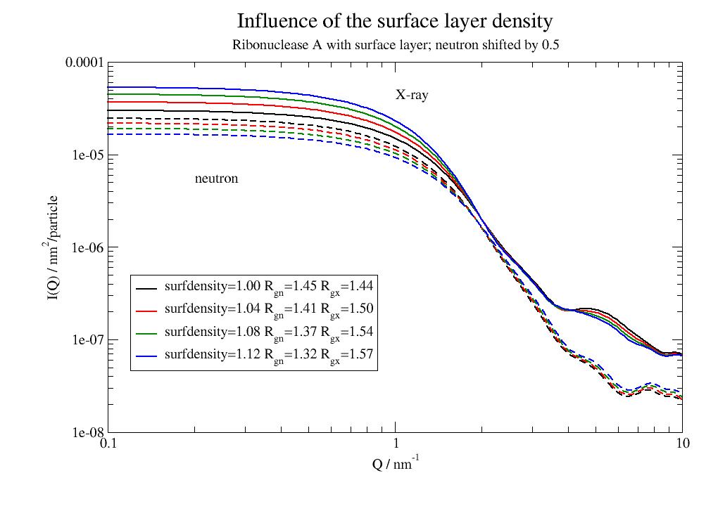
Accuracy test spherical average.
Change number of points on Fibonacci lattice for spherical average. For larger proteins Debye gets much slower (order N²), here factor 2 for error=100.
import jscatter as js

uni = js.bio.scatteringUniverse('3RN3')
# set attributes
uni.qlist=js.loglist(0.1,10,340)
uni.setSolvent(['1D2O1','0H2O1'])
u = uni.select_atoms("protein")

p=js.grace()
p.title('Spherical average accuracy')
for ii in [300,200,100,50]:
    uni.error=ii
    S=js.bio.scatIntUniv(u,mode='xray')
    p.plot(S,sy=[-1,0.1,-1],le='error=%.3g' %(ii))
uni.error=0
S=js.bio.scatIntUniv(u,mode='xray')
p.plot(S,sy=0,li=[1,1,5],le='Debye -> exact spherical average')

p.yaxis(scale='l',label=r'I(Q) / nm\S2\N/particle',min =5e-8,max=5e-5)
p.xaxis(scale='l',label='Q / nm\S-1')
p.legend(x=0.15,y=1e-6)
# p.save(js.examples.imagepath+'/accuracytestsphericalaverage.jpg')
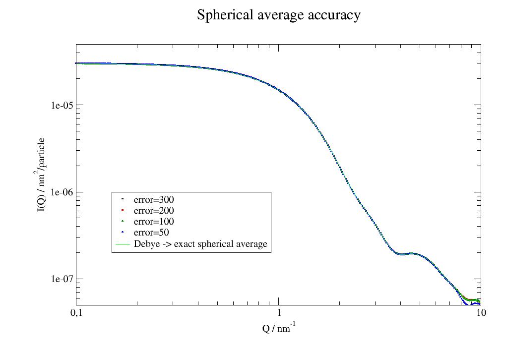
- jscatter.bio.scatIntUnivYlm(objekt, qlist=None, lmax=15, **kwargs)[source]
Neutron/Xray scattering intensity based on the Rayleigh expansion (Ylm).
Similar to CRYSOL/CRYSON (see [1]) except that we use here resolution of the atomgroup (atomic or residue). Surface layer if desired. See scatIntUniv for additional parameters and details.
- Parameters:
- objektMDAnalysis universe
Atomgroup or universe.
- qlistarray
Scattering vectors in unit 1/nm. If None or not given uni.qlist is used.
- lmaxint 15
Maximum order of spherical bessel function. For larger Q this needs to be increased. See CRYSON for a estimate what is needed.
- output‘partialAmplitudes’, default ‘normal’
Coefficients of partial waves appended as result.partialAmplitude_lm
- mode‘n’, ‘x’, ‘nvac’,’xvac’,’nshape’,’xshape’
Mode describing the type of scattering for neutron and xrays.
‘n’,’x’ -> neutron or xray scattering embedded in a solvent resulting in contrast,
‘nshape’,’xshape’ -> the shape filled with solvent (no surface layer)
‘nvac’,’xvac’ -> scattering in vacuum without solvent
- getVolume‘always’, ‘once’, ‘box’, default ‘once’
Determines volume calculation for scattering contrast.
‘always’ : For each calculation the SES/SAS volume is determined/updated using a rolling ball algorithm by
getSurfaceVolumePoints().‘once’ : Only for first call SES/SAS volume is determined using a rolling ball algorithm by
getSurfaceVolumePoints(). Some computations are speedup due to this.‘box’ : Use universe dimension to get box volume (mda.lib.mdamath.box_volume(u.dimensions)). If the box size does not change this is constant. SESVolume and SASVolume are set to the box volume.
To avoid seeing the box formfactor the solvent density in some distance of the protein/nucleic needs to be determined. See
selectSolvent().
- cubesizefloat, default None
Cube length (in units nm) for coarse graining, None means no coarse graining. For larger proteins the computation takes some time. Cubesize defines the size of a cubic grid in which atomic data as positions, formfactor and normal modes are averaged to realize a coarse graining and speedup the computation. The size should be adjusted to the protein size. This works for residue and atomic modes.
- Returns:
- dataArray[q, Fq]
Unit is nm^2/particle
Notes
An extensive description can be found in [1]. The scattering intensity is
\[I(Q) = \langle | A_a(Q) -\rho_0A_c(Q) +\delta\rho A_b(Q) |^2 \rangle_\Omega\]with \(A_a(Q)\) as particle scattering amplitude, \(A_c(Q)\) scattering amplitude of excluded solvent and \(A_b(Q)\) of the border hydration layer with densities \(\rho\) and excess hydration layer density \(\delta \rho\) . Brackets indicate orientational averaging over orientational angle \(\Omega\).
The scattering amplitudes for atoms j with atomic scattering amplitude \(f_j(Q)\) can be expressed as
\[A(Q) = \sum_{j=1}^N f_j(Q)exp(iQR_j)\]and after multipole expansion
\[A(Q) = \sum_{l=0}^{\infty}\sum_{m=-l}^{l} A_{lm}(Q)Y_{lm}(\Omega)\]\[A_{lm}(Q) = 4\pi i^l \sum_{j=1}^N f_j(Q)j_l(Qr_j)Y_{lm}^{*}(\Omega_j)\]with spherical Bessel function \(j_l(Qr_j)\) and spherical harmonics \(Y_{lm}(\Omega_j)\) . Coordinates are spherical coordinates \(r_j = (r_j,\theta_j,\phi_j) = (r_j, \Omega_j)\) .
The border hydration layer is here (different from (CRYSOL/CRYSON) depicted by dummy atoms placed at the center of the layer representing the layer volume. The dummy atoms of the excluded volume inside of the protein represent the excluded solvent at same positions as the real atoms. Inside and hydration layer dummy atoms have scattering amplitudes as described in [1] (equ 12 + 13) using atomic van der Waals volume scaled to equal the SES volume or layer volume.
References
Examples
import jscatter as js
import numpy as np
uni=js.bio.scatteringUniverse('3pgk')
uni.setSolvent('1d2o1')
uni.qlist=np.r_[0.01,0.1:2:0.2]
Sq = js.bio.scatIntUnivYlm(uni.residues)
- class jscatter.bio.scatteringUniverse(*args, **kwargs)[source]
Bases:
UniverseCreate MDAnalysis universe with atoms from PDB or simulation for neutron/Xray scattering.
scatteringUniverse()returns a MDAnalysis universe which contains proteins/DNA and solvent. It has methods e.g. for selection of parts or position analysis from MDAnalysis complemented by scattering specific methods/attributes as atomic formfactors or volume determination. Parameters describe additional scattering parameters like embedding solvent. Others are passed to MDAnalysis.universe.- Parameters:
- argspdb structure file, universe or trajectories
PDB files, PDB ID or path to trajectories to build the universe as described for MDAnalysis.universe. See MDAnalysis for different formats. Already existing local PDB files are preferred.
- biounitbool, default False
If biounit is True or above args is a PDB biounit/assembly1 with ending .pdb[biounit] as e.g.
.pdb1the biounit is downloaded, merged and used for the universe. SeemergePDBModel().- vdwradiidict
Atomic van der Waals radii (units A) passed to universe are used to calculate SES and SAS volume. The default is for protein atoms
{'H': 1.09, 'C': 1.58, 'N': 0.84, 'O': 1.3, 'S': 1.68, 'P': 1.11}These values are smaller than the vdW radii from Bondi but result in a correct SESVolume and scattering intensity. SeegetSurfaceVolumePoints().- guess_bondsMDAnalysis selection string, default=’all’
Guess bonds for atoms selected by selection string.
Bonds are needed for correct hydrogen exchange (e.g. H bonded to ‘O,N,S’ exchange with D2O to D) in neutron scattering. See hdexchange. For X-ray scattering or if all bonds are present in the topology set to False.
For trajectories with a lot of solvent, it takes time to determine solvent bonds. Selecting only parts like
guess_bonds='protein'orguess_bonds='not segid seg_1_SOL'shortcuts this. The solvent H needs to be explicitly set.hdexchangeor the atomtype to D.- assignTypesdict
Assign unknown atom type values from known atom names if the unknowns are non-standard. Some coordinate formats use non-chemical symbols (e.g. lammps uses integers), which need to be assigned some element atom types. We do this here to real atom types.
Dictionary of
{'unknownname': 'existingname'}like{'mw': 'C'}or for lamps{'1':'C','2':'H'}.The key ‘from_names’ prepends
guess_types(self.atoms.names)before above assignment ( {‘from_names’:1} ).For custom setting (not existing element) assign corresponding data for an element to
(js.bio).xrayFFatomic, .xrayFFatomicdummy, .Nscatlength, .vdwradii.- PDB file options
For assigning hydrogen, adding missing atoms, charges and optimizing positions using PDB2PQR
- addHydrogenbool, default True
Add hydrogen to atomic coordinates (only) for PDB files.
False: do not add hydrogen. Bypass all PDB options below and PDB2PQR usage.
If hydrogen is in the PDB structure or has only Cα atoms by design (e.g. coarse grained) set to False.
True:
By default
fastpdb2pqr()is used to add hydrogen in a fast mode without debumping and position optimization. Check ligands for their charge.For other formats as e.g. trajectories this option is ignored as these should contain hydrogen.
If PyMol is installed, it can be used to add hydrogen, addHydrogen=’pymol’. Pymol is maybe bit faster and add hydrogen also to ligands. No charges are added.
- debumpbool, default False
Debump added atoms, ensure that new atoms are not rebuilt too close to existing atoms.
- optbool, default False
Perform hydrogen optimization, default is not to do it, Adjusts hydrogen positions and flips certain side chains (His, Asn, Glu) as needed to optimize hydrogen bonds.
- ff‘AMBER’,’CHARMM’,’PARSE’,’TYL06’,’PEOEPB’,’SWANSON’, default: PARSE
The forcefield to use for charge assignment.
- drop_waterbool
Drop water atoms.
- phfloat, default None
pH value to use for assignment of charges. If None pH 7 is assumed but PROPKA is not used. Cite [5] [6] if using charge assignments by PROPKA.
pdb2pqr alters residue type according to the ff if the actual ph is > or < than the residue pKa. E.g. ASP -> ASH if ph< pka determined from PROPKA3 For titration see
titrationProfile()using PROPKA3.- neutralc, neutralnbool, default = False
Neutral C or N terminal.
- assign-onlybool, default: False
Only assign charges and radii - do not add atoms, debump, or optimize.
- Returns:
- UniversescatteringUniverse
See Notes for attributes and functions.
Notes
The scatteringUniverse contains proteins/DNA with/without explicit solvent, possibly in a box and has attributes as X-ray/neutron scattering amplitudes for all atoms in the universe. Parameters referring to solvent describe the embedding continuous solvent outside. Without explicit solvent a virtual surface layer and volume determination is used e.g. for PDB structures from the PDB databank or implicit solvent simulations.
Explicit solvent is in most cases simulated as protonated while neutron scattering experiments are done with D2O/H2O mixtures. This needs to be accounted by adjusting
.hdexchangefor the solvent or changing H to D for the solvent. See specific examples in Biomacromolecules (bio)Use a biological unit for calculation using PDB structures from the PDB databank. The PDB crystal structure is not always the biological unit in special for multimeric proteins. The biological assembly can be retrieved from PDB servers as e.g.https://www.ebi.ac.uk/pdbe/ . Look for biological unit or assembly. Check the structure in a PDB viewer as Pymol or VMD.
If existent the biological unit can be downloaded with .pdb1 or .pdb2 file ending, see
fetch_pdb(). The biological unit can then be merged into one model using seemergePDBModel().The scatteringUniverse has additional attributes for scattering of atoms/residues. All atoms need a defined type to determine the scattering amplitude. These attributes like fax/fan atomic formfactors are used during scattering calculations as described in
scatIntUniv().mutable Universe attributes :
qlist : array
scattering vectors in unit 1/nm.
tlist : array, optional
Times in units ps for dynamics.
solvent :
Continuous solvent embedding the atoms/universe. Saved in attribute
uni.solvent. UsesetSolvent()for details and how to change.temperature : float
Temperature in K. Use
setSolvent().solventDensity :
See and use
setSolvent().probe_radius : float 0.13
radius of the probe for surface determination in the rolling ball algorithm, See
getSurfaceVolumePoints(). The default is 0.13 [nm] for water. This reduced value (often 0.14 nm) corresponds to the reduced vdwradii of oxygen that reproduces SESVolume and results in the best protein density determination.shellThickness : float
Hydration shell thickness as surface layer thickness. Default is 0.3 nm.
point_density : int, default 5
Point density on surface (per atom) for SES and SAS calculation. See
getSurfaceVolumePoints(). \(n_{points} = 2^{2 point_density}+2\) .error : float
Determines how to calculate spherical averages (number of Fibonacci points on sphere).
amideHexFract : float 0..1
Exchangeable fraction of backbone amide -NH hydrogen
0.9 for folded proteins
For intrinsically unfolded proteins this might be higher due to improved access to the backbone. (see hdexchange to change)
histidinExchange : float 0..1
Exchangeable fraction histidine hydrogen (0.5) (see hdexchange to change)
solventDelocalisation : float, default 0.045 nm.
Debye-Waller like solvent delocalisation. See
scatIntUniv().calphaCoarseGrainRadius : float 0.342 [nm]
vdwradii for Cα only structures for coarse grained calculations. The value gives an average good approximation for the protein densities.
iscalphamodel : bool
explicitResidueFormFactorAmpl : bool
True(default) : The residue formfactor amplitude (fan/fax) is calculated explicit for each residue instead of using precalculated average values. hdexchange is included like deuterationFalse : Precalculated residue formfactors are used from
js.mda.xrayFFgroupandjs.bio.neutronFFgroup.Additional residue or monomer types can be added to the dict for coarse grained calculations e.g. of polymer bead models. In this case set
explicitResidueFormFactorAmpl=False
Atom attributes can be changed for each atom. Predefined values are OK for most folded proteins without explicit solvent. These attributes can be set for individual atoms or for groups like
urn.select_atoms('not protein and type H').deuteration =1
urn.select_atoms('not segid seg_1_SOL').hdexchange =1
rmsd : Atom delocalisation as rmsd (root mean square displacement). Debye-Waller like delocalisation of atoms that change the atomic formfactors. See
scatIntUniv()for details.heavy atom delocalisation : float, default 0.045 nm.
Crystallographic B factors are limited to \(B=8\pi^2 \langle u^2\rangle < 25 A²\) [7] leading to \(u_{max} = 0.056A\) at maximum. We use 0.045 nm with B=0.16 A² as a reasonable average.
H delocalisation : float, default 0.045 nm.
Delocalisation of non-solvent H atoms. \(\langle u^2\rangle \approx 0.21 A² \rightarrow u\approx 0.045 nm\) at 290K [8].
Change rmsd like this
uni.atoms.rmsd = 'default'  # uses [0.045,0.045]
uni.atoms.rmsd = [0.01,0.02]  # sets these values for [non H atoms, H atoms]
#  Use selection to set e.g. according to position from surface or type.
universe.select_atoms('type H and bonded type C').rmsd = 0.02
deuteration : atomic deuteration, effective only for H atoms. Fractional values are interpreted as statistical deuteration e.g. of half the atoms in an ensemble.
For residue calculation use with
uni.explicitResidueFormFactorAmpl = Trueto get updated residue formfactors accordingly.Changing deuteration updates .fans .
hdexchange: Fraction of hydrogen that exchange with solvent hydrogen for a group of atoms or individual atoms. The default is for folded proteins, Intrinsically folded may be different e.g. 1 for the backbone N-H.
To get number of exchanged H atoms
uni.atoms.hdexchange.sum()Set for atomgroup as
ag.hdexchange = (a,b,c)orag.hdexchange = 'default'witha : H bonded to O,S,sidechain N ; default 1, all exchange
b : backbone N-H : default uni.amideHexFract = 0.9
c : histidine -H : default u.histidinExchange = 0.5
A single float sets a=b=c and keyword ‘default’ sets to universe defaults. Useful for e.g a disordered part that has different backbone exchange.
Changing hdexchange updates .fans.
surfdensity : scattering length density relative to bulk for surface atoms.
Typically between 1.00 to 1.18 for proteins.
If equal 1 no surface is assumed.
Example how to set for individual atoms/residues E.g. set according to residue type or residue numbers
import jscatter as js
uni = js.bio.scatteringUniverse('3CLN')
uni.select_atoms('resname ARG HIS LYS ASP GLU').atoms.surfdensity = 1.1
protein = uni.select_atoms('protein')

# scatIntUniv uses prepScatGroups which uses getSurfaceVolumePoints to determine the surface
Sx = js.bio.scatIntUniv(protein ,mode='xray')
print('Mean universe atoms ', uni.atoms.surfdensity.mean())
print('Mean in surface atoms', protein.select_atoms('surface 1').surfdensity.mean())

# hydrophobicity scale [-4.5..4.5] dependent on residue type
md = 0.09  # maximum density in layer 9% different from bulk
for k, v in js.data.aaHydrophobicity.items():
    uni.select_atoms('resname '+k.upper()).atoms.surfdensity = 1 + md * v[0]/4.5
print('Mean universe atoms ', uni.atoms.surfdensity.mean())
print('Mean in surface atoms', protein.select_atoms('surface 1').surfdensity.mean())

# set higher exchange for backbone NH in a segment (migth be unfolded at the surface)
protein.select_atoms('resnum 33:44').atoms.hdexchange = (1, 0.7, 0.5)

# use a partial deuteration of a small domain or even individual H atoms.
# maybe partial deuteration is possible in the future
protein.select_atoms('resnum 33:44').atoms.deuteration = 1
# deuteration of 2 amino acids types
protein.select_atoms('resname ARG LYS').atoms.deuteration = 1
Immutable attributes
These atom attributes are set to defaults and updated if attributes like hdexchange, deuteration or solvent change and should not be changed manually in normal case. Residue values are appropriate averages. If needed fan/fax can be set explicit for selected atoms
uni.select_atoms('resname ARG').fans = `` or reset by ``uni.atoms.fans = 'types'.(singular/plural):
fax/faxs : atomic/residue xray formfactor amplitude, unit nm
atomic xray formfactor amplitudes \(f_j(Q)\) according to REZ et al. [2] . See
scatIntUniv()Delocalisation is taken into account exchanging \(f_i(Q)\) -> \(f^{\prime}_i(Q)\) with (\(\delta = universe.atoms.rmsd\) )
\[f^{\prime}_i(Q) = exp(-Q^2\delta^2/2) f_i(Q)\]residue formfactor amplitudes for coarse grained calculation are calculated using the Debye scattering equation with atomic positions \(r_j\) according to Yang et al. [4] if atoms are present:
\[F_a^{residue}(Q) = \big\langle \sum_{j.k} f^{\prime}_j(Q)f^{\prime}_k(Q) \frac{sin(Q(r_j-r_k))}{Q(r_j-r_k)} \big\rangle^\frac{1}{2}\]This is obviously only valid for small scattering vectors where we can neglect the atomic details and interferences in a residue, thus the real \(F_a^{residue}(Q) >0\).
Precalculated amino acid residue formfactors are stored in the dict
js.mda.xrayFFgroupandjs.bio.neutronFFgroup. Adding new ones for e.g. polymer monomersmonomerfa = js.ff.sphere(q=js.bio.QLIST, radius=1.2) monomerfa.Y = (monomer.Y/monomer.I0)**0.5 * V**2 * x_contrast**2 # valid only for small q js.bio.xrayFFgroup['ETH'] = monomerfa # naming the specific residues to use the new defined formfactor # leads to automatic usage of the new formfactor amplitude. # use select mechanism of MDAnalysis to be specific uni.residues.resnames = 'ETH' # set corresponding incoherent if needed (just as example for C2H4 monomer) # here we assume one Cα atom per residue/monomer in coarse graining. uni.residues.atoms.fi2xs = js.data.xrayFFatomic['C'][2]*2 + js.data.xrayFFatomic['H'][2] * 4
fan/fans : atomic/residue neutron formfactor amplitude unit nm
atomic neutron formfactor amplitudes which are Q independent with a scattering length according to [1] taken from https://www.ncnr.nist.gov/resources/n-lengths/list.html
Delocalisation is taken into account exchanging \(f_i(Q)\) -> \(f^{\prime}_i(Q)\) with (\(\delta = universe.atoms.rmsd\) )
\[f^{\prime}_i(Q) = exp(-Q^2\delta^2/2)]f_i(Q)\]residue scattering is calculated as for fax based on atomic scattering amplitudes..
fi2n/fi2ns : neutron incoherent scattering amplitude squared, unit nm². Same source as fan.
fi2x/fi2xs : xray incoherent scattering amplitude squared according to [3] (compton scattering), unit nm².
posnm : atom/residue center of geometry positions in unit nm. MDAnalysis uses Å in .position. posnm is for convenience to get 1/nm wavevectors.
surface : name of surface, to test if atoms belong to surface atoms. (Maybe later different surfaces)
surfdata : surface atom data as [surface area, surface volume, shell volume, 3x surface area mean position]
vdWradiinm : vdWradii in nm as defined in js.data.vdwradii
Set default values dependent on .solvent using See
setSolvent().xsld : solvent xray scattering length density, unit 1/nm²=nm/nm³
edensity : solvent electron density, unit e/nm³
bcDensitySol : solvent neutron scattering length density, unit 1/nm²=nm/nm³
b2_incSol : solvent neutron incoherent scattering length density squared, unit 1/nm=nm²/nm³
d2oFract : solvent d/h mol fraction
d2omassFract : solvent d/h mass fraction
References
[1]Neutron scattering lengths and cross-sections V. F. Sears Neutron News, 3, 26-37 (1992) https://doi.org/10.1080/10448639208218
[2]REZ et al.Acta Cryst. A50, 481-497 (1994)
[3]A new analytic approximation to atomic incoherent X-ray scattering intensities. J. THAKKAR and DOUGLAS C. CHAPMAN Acta Cryst. (1975). A31, 391
[4]A Rapid Coarse Residue-Based Computational Method for X-Ray Solution Scattering Characterization of Protein Folds and Multiple Conformational States of Large Protein Complexes S. Yang, S. Park, L. Makowski, B. Roux Biophysical Journal 96, 4449–4463 (2009) doi: 10.1016/j.bpj.2009.03.036
[5]An improved method for calculating the contribution of solvent to the X-ray diffraction pattern of biological molecules R. D. B. Fraser, T. P. MacRae and E. Suzuki J. Appl. Cryst. (1978). 11, 693-694 https://doi.org/10.1107/S0021889878014296
[6]What can x-ray scattering tell us about the radial distribution functions of water? Jon M. Sorenson, Greg Hura, Robert M. Glaeser, et al. J. Chem. Phys. 113, 9149 (2000); https://doi.org/10.1063/1.1319615
[7]How large B-factors can be in protein crystal structures. Carugo et al BMC Bioinformatics 19, 61 (2018). https://doi.org/10.1186/s12859-018-2083-8
[8]Hydrogen atoms in proteins: Positions and dynamics Engler, Ostermann, Niimura, Parak PNAS 100, 10243 (2003) https://doi.org/10.1073/pnas.1834279100
Examples
Load pdb protein structure from the PDB data bank by ID to scatteringUniverse. The pdb file is corrected and hydrogen is added automatically. The protein structure including H is saved to 3rn3_h.pdb.
import jscatter as js
import numpy as np

uni = js.bio.scatteringUniverse('3rn3')
uni.view()
uni.setSolvent('1d2o1')
uni.qlist = js.loglist(0.1, 5, 100)
# calc scattering both here in D2O
S = js.bio.nscatIntUniv(uni.select_atoms('protein'))
S = js.bio.xscatIntUniv(uni.select_atoms('protein'))

p = js.grace()
p.title('N scattering solvent matching')
p.yaxis(scale='l', label=r'I(Q) / nm\S2\N/particle')
p.xaxis(scale='l', label='Q / nm\S-1')

for x in np.r_[0:0.5:0.1]:
    uni.setSolvent([f'{x:.2f}d2o1',f'{1-x:.2f}h2o1' ])
    Sn = js.bio.nscatIntUniv(uni.select_atoms('protein'))
    p.plot(Sn, le=f'{x:.2f} D2O')

p.legend()
# p.save(js.examples.imagepath+'/biosolventmatching.jpg', size=(2, 2))
Load existing PDB file (the one with H from above)
# reload the generated structurestructure later with hydrogen using the local saved structure.
uni2 = js.bio.scatteringUniverse('3rn3_h.pdb',addHydrogen=False)
uni2.view()
A scatteringUniverse with a complete trajctory from MD simulation is created. The PSF needs atomic types to be guessed from names to identify atoms in the used format. You may need to install MDAnalysisTests to get the files.( python -m pip install MDAnalysisTests)
It migh be nesserary to transform the box that the protein is not crossing boundaries of the universe box.
from MDAnalysisTests.datafiles import PSF, DCD
import jscatter as js
import numpy as np
import MDAnalysis as mda
from MDAnalysis.topology.guessers import guess_types

upsf1 = js.bio.scatteringUniverse(PSF, DCD, assignTypes={'from_names':1})
upsf1.view(frames="all")

upsf1.setSolvent('1d2o1')
upsf1.qlist = js.loglist(0.1, 5, 100)

Sqtraj = js.dL()

# select protein and not the solvent if this is present
protein = upsf1.select_atoms('protein')

if 0:
    # only if needed to avoid crossing boundaries
    # add a transform that puts the protein into the center of the box and wrap the solvent into the new box
    # for details see  MDAnalysis Trajectory transformations
    protein = upsf1.select_atoms('protein')
    not_protein = upsf1.select_atoms('not protein')
    transforms = [trans.unwrap(protein),
                  trans.center_in_box(protein, wrap=True),
                  trans.wrap(not_protein, compound='fragments')]

# now loop over trajectory
for ts in upsf1.trajectory[2::13]:
    Sq = js.bio.nscatIntUniv(protein)
    Sq.time = upsf1.trajectory.time
    print(Sq.RgInt)
    Sqtraj.append(Sq)

# show
p = js.grace()
p.title('N scattering along ADK trajectory')
p.subtitle(r'change in R\sg\N; no change of SES volume')
p.yaxis(scale='l',label=r'I(Q) / nm\S2\N/particle')
p.xaxis(scale='l',label='Q / nm\S-1')
p.plot(Sqtraj,le=r't= $time ps; R\sg\N=$RgInt nm; V\sSES\N=$SESVolume nm\S3')
p.legend(x=0.15,y=1e-5,charsize=0.7)
# p.save(js.examples.imagepath+'/uniformfactorstraj.jpg', size=(2, 2))
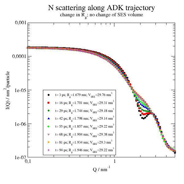
scatteringUniverse does the same as this in MDAnalysis.
u = mda.Universe(PSF, DCD)
# determine types from names
u.atoms.types = guess_types(u.atoms.names)
u.atoms.guess_bonds(vdwradii={'H': 1.09, 'C': 1.58, 'N': 0.84, 'O': 1.3, 'S': 1.68, 'P': 1.11})
# add scattering attributes
upsf2 = js.bio.scatteringUniverse(u, addHydrogen=False, guess_bonds=False)
Examples for PDB structures without explicit solvent for small angle scattering
The example shows the validity of residue coarse graining up to around 3/nm. With coarse graining in cubes (cubesize) the approximation seems best. This might be useful to speed up computations that take long (e.g. ISF at low Q)
There is basically no difference between precalculated and averaged residue formfactors and explicit calculated residue formfactors for each residue (uni.explicitResidueFormFactorAmpl = True) The explicit ones include better deuteration of specific atoms.
Cα models loose some precision in volume respectivly in forward scattering. C-alpha models need a .calphaCoarseGrainRadius = 0.342 nm because of the missing atoms. In addition, the mean residue position is not the C-alpha position. We use 0.342 nm as a good average to get same forward scattering over a bunch of proteins (see example_bio_proteinCoarseGrainRadius.py).
import jscatter as js

# first get and create the biological unit ('.pdb1') of alcohol dehydrogenase (tetramer, 144 kDa)
adh = js.bio.fetch_pdb('4w6z.pdb1')
# the 2 dimers in are in model 1 and 2 and need to be merged into one.
adhmerged = js.bio.mergePDBModel(adh)

# Ribonuclease A and Phosphoglycerate kinase are monomers and can be used without modifications.
# 3pgk has a Mg atom that is misinterpreted (as M), to use it we add this
vdwradii = {'M': js.data.vdwradii['Mg'] * 10}  # in A

p = js.grace(1, 1.4)
p.multi(3, 2, vgap=0, hgap=0)
for c, pdbid in enumerate(['3rn3', '3pgk', adhmerged]):
    # load from pdb id, scatteringUniverse adds hydrogens automatically
    uni = js.bio.scatteringUniverse(pdbid, vdwradii=vdwradii)
    uni.setSolvent('1d2o1')
    uni.qlist = js.loglist(0.1, 9.9, 200)
    u = uni.select_atoms("protein")
    ur = u.residues

    S = js.bio.nscatIntUniv(u)
    Sx = js.bio.xscatIntUniv(u)

    # use an averaging in cubes filled with the atoms, cubesize approximates residue size
    Scu = js.bio.nscatIntUniv(u, cubesize=0.6)
    Sxcu = js.bio.xscatIntUniv(u, cubesize=0.6)

    # use now the precalculated formfactors on residue level coarse graining
    uni.explicitResidueFormFactorAmpl = False  # default
    Sr = js.bio.nscatIntUniv(ur)
    Sxr = js.bio.xscatIntUniv(ur)

    # calc residue formfactors explicit (not precalculated)
    # useful for changes of residue deuteration or backbone N-H exchange of IDP
    uni.explicitResidueFormFactorAmpl = True
    Ser = js.bio.nscatIntUniv(ur)
    Sxer = js.bio.xscatIntUniv(ur)

    # create a C-alpha pdb file and then the Ca-only universe for calculation
    ca = uni.select_atoms('name CA')
    ca.write('pdb_ca.pdb')
    # addHydrogen=False prevents addition of 4H per C atom
    unica = js.bio.scatteringUniverse('pdb_ca.pdb', addHydrogen=False)
    # To use precalculated residue formfactors explicit... should be False
    unica.explicitResidueFormFactorAmpl = False
    unica.setSolvent('1d2o1')
    unica.qlist = js.loglist(0.1, 10, 200)
    uca = unica.residues
    Sca = js.bio.nscatIntUniv(uca, getVolume='now')
    Sxca = js.bio.xscatIntUniv(uca)

    p[2 * c].plot(S, li=[1, 2, 1], sy=0, le='atomic')
    p[2 * c].plot(Scu, li=[1, 2, 5], sy=0, le='atomic in cubes')
    p[2 * c].plot(Sr, li=[1, 2, 2], sy=0, le='res pre')
    p[2 * c].plot(Ser, li=[3, 2, 3], sy=0, le='res ex')
    p[2 * c].plot(Sca, li=[1, 2, 4], sy=0, le='Ca model')
    p[2 * c].legend(x=1, y=8e-3, charsize=0.8)
    p[2 * c].text(x=0.15, y=1e-7, charsize=1, string=pdbid)

    p[2 * c + 1].plot(Sx, li=[1, 2, 1], sy=0, le='atomic')
    p[2 * c + 1].plot(Sxcu, li=[1, 2, 5], sy=0, le='atomic in cubes')
    p[2 * c + 1].plot(Sxr, li=[1, 2, 2], sy=0, le='res pre')
    p[2 * c + 1].plot(Sxer, li=[3, 2, 3], sy=0, le='res ex')
    p[2 * c + 1].plot(Sxca, li=[1, 2, 4], sy=0, le='Ca model')
    p[2 * c + 1].legend(x=1, y=8e-3, charsize=0.8)
    p[2 * c + 1].text(x=0.15, y=1e-7, charsize=1, string=pdbid)

    p[2 * c].xaxis(label='', ticklabel=False, scale='log', min=1e-1, max=9.9)
    p[2 * c + 1].xaxis(label='', ticklabel=False, scale='log', min=1e-1, max=9.9)
    p[2 * c].yaxis(label='F(Q)', ticklabel='power', scale='log', min=3e-8, max=8e-3)
    p[2 * c + 1].yaxis(ticklabel=False, scale='log', min=3e-8, max=8e-3)

p[2 * c].xaxis(label=r'Q / nm\S-1', ticklabel=True, scale='log', min=1e-1, max=9.9)
p[2 * c + 1].xaxis(label=r'Q / nm\S-1', ticklabel=True, scale='log', min=1e-1, max=9.9)
p[0].subtitle('neutron scattering')
p[1].subtitle('Xray scattering')
p[0].title(' ' * 30 + 'Comparison of formfactors with different resolution')
# p.save(js.examples.imagepath+r'/uniformfactors.jpg', size=(700/300, 1000/300))
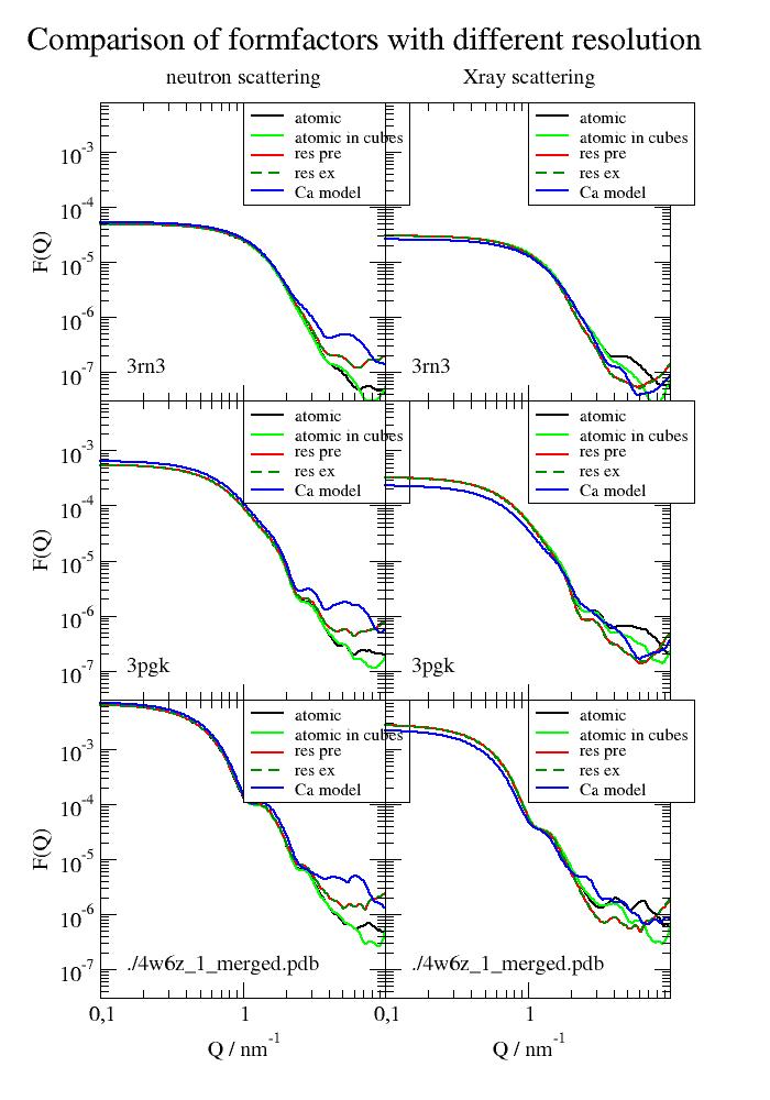
- property b2_incSol
Incoherent neutron scattering length density solvent.
- property bcDensitySol
Coherent neutron scattering length density of solvent.
- property boxVolume
Volume of universe box in A³
- property d2oFract
D2O number fraction in solvent.
- property edensitySol
Electron density solvent in e/nm³
- guess_bonds(guess_bonds='all', vdwradii=None)[source]
Guess bonds according to distance between atoms.
Bonds between atoms are created, if the two atoms are within \(d < f \cdot (R_1 + R_2)\) of each other, where \(R_{1,2}\) are the VdW radii of the atoms and \(f=0.55\) is an ad-hoc fudge_factor. This is the same algorithm that VMD uses but with f=0.6.
- Parameters:
- guess_bondsMDAnalysis selection string, default=’all’
Guess bonds for atoms selected by selection string.
Bonds are needed for correct hydrogen exchange (e.g. H bonded to ‘O,N,S’ exchange with D2O to D) in neutron scattering. See hdexchange. For X-ray scattering or if all bonds are present in the topology set to False.
For trajectories with a lot of solvent, it takes time to determine solvent bonds. Selecting only parts like
guess_bonds='protein'orguess_bonds='not segid seg_1_SOL'shortcuts this. The solvent H needs to be explicitly set.hdexchangeor the atomtype to D.- vdwradiidict, default None
Dictionary with {name:value[A]} pairs for vdWaals radii.
- Returns:
- None, bonds are created as atomAttribute
bonds.
- None, bonds are created as atomAttribute
Notes
Atomic van der Waals radii (units A) passed to universe are used to identify bonds between atoms using the universe.guess_bonds method of MDAnalysis.
The default radii are according to https://en.wikipedia.org/wiki/Atomic_radii_of_the_elements_(data_page)#Van_der_Waals_radius (mainly Bondi reference, default of MDAnalysis). These values are larger than the radii for SESvolume calculation (
getSurfaceVolumePoints()) to identify all bonds.
- property numDensitySol
Number density solvent in 1/nm³
- property qlist
Scattering vectors
- setSolvent(solvent=None, density=None, temperature=None, numDensity=None, units='mol')[source]
Set solvent emdedding the universe to calculate scattering lengths and contrast.
Usage only for changing solvent. Other parameters changed automatically.
- Parameters:
- solventlist of string
Describes solvent composition with molar fractions. If None universe.solvent is used.
A chemical formula with fraction+[lettercode+number]+…..
e.g.’D2O1’ or ‘H2O1’ for water and heavy water
[‘0.6D2O1’,’0.4H2O1’] for a mixture of 0.6 hwater and 0.4 water by mol fraction
[‘6D2O1’,’4H2O1’] for a mixture of 6 hwater and 4 water as mixed mol
default is pure h2o
- densityoptional, default=None, float
Density of the solvent in units g/cm³.
Explicit given values force the density to be different from tabulated values!
By default (None) tabulated values according to formel.waterdensity as given in solvent are use.
See :py:func:’jscatter.formel.waterdensity’ for specific references.
- numDensity: optional, default=None, float
Number density of solvent molecules in units 1/nm³.
Forces scaling of related values to different number density e.g. in a simulation box.
Overrides density above and is intended only for simulation boxes. - 0 : resets to above density values. - None : water with components as given in universe.solvent is used.
This is the default for protein scattering from PDB structures (like implicit solvent). See :py:func:’jscatter.formel.waterdensity’ for specific references.
float: For explicit solvent universes from MD simulation the values gives the total number density of all solvent molecules used in the MD simulation.
- temperaturefloat
Temperature of the universe in units K.
- units‘mol’
Units used in solvent as mol or mass. Anything except ‘mol’ (default) is mass fraction .
e.g. 1l Water with 123mmol NaCl [‘55.5H2O1’,’0.123Na1Cl1’]
See :py:func:’jscatter.formel.scatteringLengthDensityCalc’.
- Returns:
- Sets universe attributes
solventDensity, numDensitySol, bcDensitySol, edensitySol, b2_incSol,d2oFract, xsldSol
Notes
scatteringLengthDensityCalc()is used to calc solvent scattering length (units=mol).For a simulation box with water it is important to have the correct water numDensity some distance away from the protein surface (outside of the hydration layer) to get the right contrast to the embedding solvent. Simulation boxes have not always the correct waterdensity. This is automatically taken into account.
For PDB structures or simulation with implicit solvent the density is waterdensity.
For simulation boxes the numberdensity of the initial box is usually fixed and not changed (constant volume simulation over constant pressure).
If the initial equal distributed water forms a hydration layer with higher density around the protein, consequently the density outside the hydration layer must decrease. To correctly determine the contrast we need the numberdensity of the solvent outside of the hydration layer.
We can extract this by selecting water some distance away from the protein surfece. In the same way we can approximate the numberdensity in the hydration layer.
- view(select='all', frames=None, viewer='')[source]
View the actual configuration in a selected viewer.
- Parameters:
- selectstring, default = ‘all’
Selection string as in select_atoms.
- framesarray-like or slice or FrameIteratorBase or str, optional
An ensemble of frames to write. The ensemble can be a list or array of frame indices, a mask of booleans, an instance of
slice, or the value returned when a trajectory is indexed. By default, frames is set toNoneand only the current frame is written. If frames is set to “all”, then all the frame from trajectory are written.- viewer‘pymol’, ‘vmd’, ‘chimera’, or full path
Viewer to show pdb structure.
If the programm is in the PATH the short name is enough.
The full path can be specified.
default is to use the first existing.
Examples
Normal modes are just used to generate a trajectory.
import jscatter as js

# view single structure
uni = js.bio.scatteringUniverse('3RN3.pdb')
uni.view(select='protein')

# normal mode anmation saved as trajectory
uni = js.bio.scatteringUniverse(js.examples.datapath+'/arg61.pdb',addHydrogen=False)
u = uni.select_atoms("protein and name CA")
nm = js.bio.NM(u, cutoff=10)
moving = nm.animate([6,7,8,9], scale=30)  # as trajectory

# view trajectory
moving.view(viewer="pymol", frames="all")

# animate and show
nm.animate([6, 7, 8, 9], scale=30).view(viewer="pymol", frames="all")
- property xsldSol
X-ray scattering length of solvent.
- jscatter.bio.titrationProfile(atomgroup, select='protein', propkaargs=['--quiet'], write_pka=False)[source]
Get charges and pKa of residues using propka3.
PROPKA predicts the pKa values of ionizable groups in proteins and protein-ligand complexes (version 3.1 and later) based on the 3D structure. We use PROPKA3 from the Jensen group as described in [1] and [2]. The original source is at https://github.com/jensengroup/propka. Please cite PPROPKA if you use this function.
- Parameters:
- atomgroupatomgroup
MDAnalysis atomgroup
- selectstring
MDAnalysis selection string used on atomgroup.
- propkaargslist of string
Arguments passed to propka3
- write_pkabool
Write the output file of propka analysis including
per residue analysis
pKa prediction list
free energy
Protein charge of folded and unfolded state as a function of pH (unfolded , folded)
pI folded , unfolded
- Returns:
- titrationprofile, charged_residuesdataArray, dict
Titration profile for unfolded and folded state
Charge of residues as dict with items {resnum : [charge, pka value, buried surface fraction]}
References
[1]Improved Treatment of Ligands and Coupling Effects in Empirical Calculation and Rationalization of pKa Values Sondergaard, Chresten R., Mats HM Olsson, Michal Rostkowski, and Jan H. Jensen Journal of Chemical Theory and Computation 7, no. 7 (2011): 2284-2295. doi:10.1021/ct200133y
[2]PROPKA3: consistent treatment of internal and surface residues in empirical pKa predictions. Olsson, Mats HM, Chresten R. Sondergaard, Michal Rostkowski, and Jan H. Jensen Journal of Chemical Theory and Computation 7, no. 2 (2011): 525-537. doi:10.1021/ct100578z
Examples
import jscatter as js

uni = js.bio.scatteringUniverse('3rn3')
titprof, rescharges = js.bio.titrationProfile(uni.atoms, propkaargs='')

p = js.grace()
p.plot(titprof._ph,titprof._unfolded,le='unfolded')
p.plot(titprof._ph,titprof._folded,le='folded')
p.plot([titprof.isoelectricPoint[0]]*2, [-20,20],li=1,sy=0,le='pI folded')
p.plot([titprof.isoelectricPoint[1]]*2, [-20,20],li=[3],sy=0,le='pI unfolded')
p.xaxis(label='pH')
p.yaxis(label='total charge')
p.legend(x=10,y=18)
p.title('Ribonuclease A charge profile')
#p.save(js.examples.imagepath+'/titrationRibonuclease.jpg',)
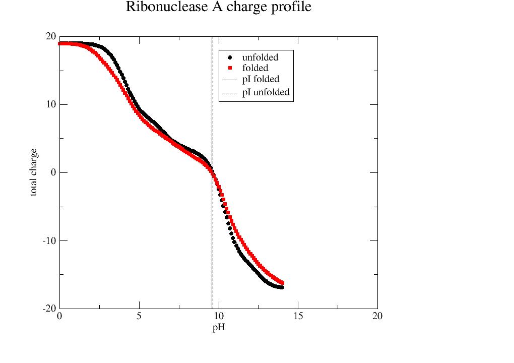
- class jscatter.bio.vibNM(atomgroup, k_b=418, k_nb=None, vdwradii=None, cutoff=13, rigidgroups=None)[source]
Bases:
NMMass weighted vibrational normal modes like ANMA modes.
Modes are mass weighted elastic normal modes with eigenvalue \(\omega_i\) and frequency \(f_i = \omega^{1/2}/(2\pi)\).
See
ANMA()for details.- Parameters:
- atomgroupMDAnalysis atomgroup
Atomgroup or residues for normal mode analysis If residues the Cα atoms for aminoacids and for others the atom closest to the center is choosen.
The total mass of a residue is used for the weight. For Ca only universes the mass is consequently roughly 10times to small and needs to be increased to deliver reasonable results.
- vdwradiifloat, dict, default=3.8
vdWaals radius used for neighbor bond determination. The default corresponds to Cα backbone distance. If dict like js.data.vdwradii these radii are used for the specified atoms.
- cutofffloat, default 13
Cutoff for nonbonded neighbor determination with distance smaller than cutoff in units A. See [2] for comparison.
- k_bfloat, default = 418.
Bonded spring constant between atomgroup elements in units g/ps²/mol.
418 g/ps²/mol = 694 pN/nm = 1(+-0.5) kcal/(molA²)as mentioned in [2] to reproduce a reasonable protein frequency spectrum.- k_nbfloat, default = None.
Non-bonded spring constant in same units as k_b. If None,
k_nb = k_b.- rigidgroupsAtomGroup or list of AtomGroups
Rigid group or groups of atoms in argument atomgroups. Atoms in Atomgroup will get bonds to all others of strength rigidfactor*k_b with .rigidfactor=2 to make the group internaly more rigid.
e.g. rigid = uni.select_atoms(‘protein and name CA’)[:13].atoms
- Attributes:
- _See
NMfor additional attributes.
- _See
- Returns:
- Normal Mode Analysis objectvibNM
Object can be indexed do get a specific Mode object representing real space displacements in unit A. Trivial modes of translation and rotation are [0..5] while the first nontrivial mode is 6.
Notes
Mass weighted normal modes are solutions of the equation of motion
\[M\ddot{r} = K(r-r_0)\]with diagonal mass matrix \(M\) and force constant matrix \(K\). For coarse grained NM the mass of the coarse grains is relevant (e.g. residue based the residue mass).
In Mass weighted coordinates \(\tilde{r} = \sqrt{M}r\) this leads to
\[\ddot{\tilde{r}} = \tilde{K}(\tilde{r}-\tilde{r}_0)\]using \(\tilde{K} = \sqrt{M}^{-1}K\sqrt{M}^{-1}\)
The equation is solved by weighted eigenmodes \(\hat{v}_i\) and eigenvalues \(\omega_i^2\). Weighted eigenmodes \(\hat{v}_i\) are orthogonal \(\hat{v}_i \cdot \hat{v}_i= \delta_{i,j}\) and \(|\hat{v}_i|=1\). Unweighted modes \(v = \hat{v}_i/\sqrt{M}\) are not orthogonal and \(|v_i|\neq 1\).
For a distortion with amplitude A along mode i from equillibrium the particles oscillates along the solution \(r(t) = r_0 + A \hat{v}_i cos(\omega_i t + \phi_i)\) with random phase \(\phi_i\) [4]. Correlation of modes would fix the phase.
In equillibrium thermal motions induce fluctuations with amplitude \(d_i = A\tilde{v}_i = \sqrt{kT/(m_a\omega_j^2)}\hat{v}_i\).
For a detailed description see [3]-[4] .
References
[1]Doruker P, Atilgan AR, Bahar I. Dynamics of proteins predicted by molecular dynamics simulations and analytical approaches: Application to a-amylase inhibitor. Proteins 2000 40:512-524.
[2] (1,2)Atilgan AR, Durrell SR, Jernigan RL, Demirel MC, Keskin O, Bahar I. Anisotropy of fluctuation dynamics of proteins with an elastic network model. Biophys. J. 2001 80:505-515.
[3]Harmonicity in slow protein dynamics. Retrieved from Hinsen, K., Petrescu, A.-J., Dellerue, S., Bellissent-Funel, M.-C., & Kneller, G. R. . Chemical Physics, 261(1–2), 25–37. (2000) https://doi.org/10.1016/S0301-0104(00)00222-6
[4] (1,2)Normal Mode Theory and Harmonic Potential Approximations. In Normal Mode Analysis: Theory and Applications to Biological and Chemical Systems (pp. 1–16). Hinsen, K. (2005). https://doi.org/10.1201/9781420035070.ch1
Examples
import jscatter as js
uni=js.bio.scatteringUniverse('3pgk')
u = uni.select_atoms("protein and name CA")
nm = js.bio.vibNM(u)
# get first nontrivial mode 6
nm6 = nm[6]
nm6.rmsd  # mode rmsd displacement
- eFC(i)
Effective force constant \(k_{eff} = m_{eff} \omega_i^2 = m_{eff} (2\pi f_{i}^2)\) in units g/ps²/mol = 1.658 pN/nm.
Equivalent force constant of a 1dim oscillator along the respective normal mode.
- eM(i)
Effective mass \(m_{eff} = |\hat{v}|^2/|v|^2\) of a mode in atomic mass units g/mol.
Equivalent mass of a 1dim oscillator along the respective normal mode v.
- effectiveForceConstant(i)[source]
Effective force constant \(k_{eff} = m_{eff} \omega_i^2 = m_{eff} (2\pi f_{i}^2)\) in units g/ps²/mol = 1.658 pN/nm.
Equivalent force constant of a 1dim oscillator along the respective normal mode.
- jscatter.bio.xscatIntUniv(objekt, qlist=None, **kwargs)[source]
Xray scattering intensity with contrast to solvent.
See See
scatIntUniv()with mode=’x’ for details.
- jscatter.bio.hullRad(pdb, output=True)[source]
Dtrans, Drot, S and more from PDB structure using HullRad for H2O at T=20 C.
From the abstract of [1] :
… to accurately predict the hydrodynamic properties of molecular structures. This method uses a convex hull model to estimate the hydrodynamic volume of the molecule and is orders of magnitude faster than common methods. It works well for both folded proteins and ensembles of conformationally heterogeneous proteins and for nucleic acids. Because of its simplicity and speed, the method should be useful for the modification of computer-generated, intrinsically disordered protein ensembles and ensembles of flexible, but folded, molecules in which rapid calculation of experimental parameters is needed.
Quality of the data is comparable to HYDROPRO [2] but only scalar values are calculated. For calculation of the 6x6 diffusion tensor see
runHydropro()- Parameters:
- pdbstring or IOString from MDA PDBWriter.
Protein or DNA
- Returns:
- resultdict
Notes
All values are calculated for H2O at T=20 degree Celsius (see [1])
Coefficients keys, meaning and units (see [1] for detailed explanation)
'Dt'         Dt                        cm^2/s;   translational diffusion coefficient
'Rht'        Rh from Dt                Angstroms
'Dr'         Dr                        s^-1;     rotational diffusion coefficient
'Rhr'        Rh  from Dr               Angstroms
'AA'         number Amino Acids
'NA'         number Nucleotides
'GL'         number Saccharides
'DT'         number Detergents
'M'          mass                      g/mol
'vbar_prot'  v_bar specific volume     mL/g
'Ro'         Ro(Anhydrous)             Angstroms
'Rg'         Rg(Anhydrous)             Angstroms
'Dmax'       Dmax                      Angstroms
'a_b_ratio'  axial Ratio               equivalent prolate ellipsoid axial ratio
'ffo_hyd_P'  f/fo                      Perrin friction factor
's'          s                         sec
'tauC'       tauC (from Rhr)           ns;  isotropic rotational correlation time (NMR)
'asphr'      Asphericity from Gyration Tensor
Biological unit Use a biological unit for calculation. The crystal structure is not always the biological unit but these can be retrieved from PDB servers as e.g.https://www.ebi.ac.uk/pdbe/ . See below examples and
mergePDBModel().References
[1] (1,2,3)HullRad: Fast Calculations of Folded and Disordered Protein and Nucleic Acid Hydrogynamic Properties Fleming, PJ and Fleming, KG “”, Biophysical Journal, 2018, 114:856-869, DOI: 10.1016/j.bpj.2018.01.002
[2]Calculation of hydrodynamic properties of globular proteins from their atomic-level structure Garcıa De La Torre, J., M. L. Huertas, and B. Carrasco. Biophys. J. 78:719–730, (2000)
Examples
Based on pdb file
import jscatter as js
# give existing filename
res = js.bio.hullRad('3pgk.pdb')
For a universe from MDAnalysis. hullRad strips non protein atoms.
import jscatter as js
uni = js.bio.scatteringUniverse('3pgk')
res = js.bio.hullRad(uni.select_atoms('protein'))
# Dtrans/Drot with conversion to nm²/ps and 1/ps
Dtrans = res['Dt'] * 1e2
Drot = res['Dr'] * 1e-12
Build biological unit for a tetramer using
mergePDBModel()from downloaded biological assemblyimport jscatter as js # first get and create the biological unit ('.pdb1') of alcohol dehydrogenase (tetramer, 144 kDa) adh = js.bio.fetch_pdb('4w6z.pdb1') # the 2 dimers in are in model 1 and 2 and need to be merged into one. adhmerged = js.bio.mergePDBModel(adh) uni = js.bio.scatteringUniverse(adhmerged) res = js.bio.hullRad(uni.select_atoms('protein')) # Dtrans/Drot with conversion to nm/ps and 1/ps Dtrans = res['Dt'] * 1e2 Drot = res['Dr'] * 1e-12 Dq = js.bio.diffusionTRUnivYlm(uni,Dtrans=Dtrans,Drot=Drot)