8. dynamic

Models describing dynamic processes mainly for inelastic neutron scattering but also DLS or XCPS in time domain.

Models in the time domain have a parameter t for time. -> intermediate scattering function $I(t,q)$
Models in the frequency domain have a parameter w for frequency and _w appended. -> dynamic structure factor $S(w,q)$

Models in time domain can be transformed to frequency domain by time2frequencyFF() implementing the Fourier transform $S(w,q) = F(I(t,q))$.

In time domain the combination of processes $I_i(t,q)$ is done by multiplication, including instrument resolution $R(t,q)$:

$I(t,q)=I_1(t,q)I_2(t,q)R(t,q)$.

# multiplying and creating new dataArray
I(t,q) = js.dA( np.c[t, I1(t,q,..).Y*I2(t,q,..).Y*R(t,q,..).Y ].T)

In frequency domain it is a convolution, including the instrument resolution.

$S(w,q) = S_1(w,q) \otimes S_2(w,q) \otimes R(w,q)$.

conv=js.formel.convolve
S(w,q)=conv(conv(S1(w,q,..),S2(w,q,..)), res(w,q,..), normB=True)      # normB normalizes resolution

res(w,q,..) might be a measurement or the result of a fit to a measurement. A fitted measurement assumes a continuous extrapolation at the edges and a smoothing, while a measurement is cut at the edges to zero and contains noise.

Time to frequency FFT

FFT from time domain by time2frequencyFF() may include the resolution where it acts like a window function to reduce spectral leakage with vanishing values at $t_{max}$. If not used $t_{max}$ needs to be large (see tfactor) to reduce spectral leakage.

shiftAndBinning

The last step is to shift the model spectrum to the symmetry point of the instrument as found in the resolution measurement and optional binning over frequency channels. Both is done by shiftAndBinning().

Usage example

Example

Let us describe the diffusion of a particle inside a diffusing invisible sphere by mixing time domain and frequency domain.

resolutionparameter={'s0':5,'m0':0,'a0':1,'bgr':0.00}
w = np.r_[-100:100:0.5]
resolution = js.dynamic.resolution_w(w,**resolutionparameter)
# model
def diffindiffSphere(w,q,R,Dp,Ds,w0,bgr):
    # time domain with transform to frequency domain
    diff_w = js.dynamic.time2frequencyFF(js.dynamic.simpleDiffusion,resolution,q=q,D=Ds)
    # last convolution in frequency domain, resolution is already included in time domain.
    Sx = js.formel.convolve(js.dynamic.diffusionInSphere_w(w=w,q=q,D=Dp,R=R),diff_w)
    Sxsb = js.dynamic.shiftAndBinning(Sx,w=w,w0=w0)
    Sxsb.Y += bgr       # add background
    return Sxsb
#
Iqw=diffindiffSphere(w=w,q=5.5,R=0.5,Dp=1,Ds=0.035,w0=1,bgr=1e-4)

For more complex systems e.g a number x of diffusing hydrogen’s and a number y of fixed oxygen and carbons different scattering length and changing fraction of contributing atoms (with scattering length) has to be included just by adding a corresponding factor. This factor can e.g. be determined from an atomic structure.

Accordingly, if desired, the mixture of coherent and incoherent scattering needs to be accounted for by corresponding scattering length. This additionally is dependent on the used instrument e.g. for spin echo only 1/3 of the incoherent scattering contributes to the signal. An example model for protein dynamics is given in Protein incoherent scattering in frequency domain.

A comparison of different dynamic models in frequency domain is given in examples.

8.1. Transform between domains

`time2frequencyFF`(timemodel, resolution[, w, ...])	Fast Fourier transform from time domain to frequency domain for inelastic neutron scattering.
`frequency2timeFF`(data[, resolution_t, dt, ...])	Fourier transform from frequency domain (experiment) to time domain for inelastic neutron scattering.
`shiftAndBinning`(data[, w, w0, Qname])	Shift w spectrum and average (binning) in intervals.
`convert_e2w`(data[, T, unit, replaceZero])	Convert energy or 1/ps units to frequency 1/ns units and correct for detailed balance.
`mirror_w`(data[, emin])	Mirrors w spectra from energy gain to energy loss side.
`convolve`(A, B[, mode, normA, normB])	Convolve A and B with proper tracking of the output X axis mainly for inelastic scattering.

`getHWHM`(data[, center, gap])	Find half width at half maximum (left/right) of a distribution around center.
`dynamicSusceptibility`(data, Temp)	Transform from S(w,q) to the imaginary part of the dynamic susceptibility.
`k`	Boltzmann constant in meV/K
`h`	Planck constant in µeVns = meVps
`hbar`	h/2π reduced Planck constant in µeVns = meVps
`u2Debye`(T, thetaD[, amass])	u2 based on Debye density of states.

8.2. Time domain

`resolution`(t[, s0, m0, s1, m1, s2, m2, s3, ...])	Resolution in time domain as multiple Gaussians for inelastic measurement as back scattering or time of flight instrument.
`transDiff`(t, q, D)	Translational diffusion intermediate scattering function in t domain.
`simpleDiffusion`(t[, gamma, q, D, s, beta, type])	Intermediate scattering function [g1(t)] for diffusing particles from distribution of relaxation rates.
`doubleDiffusion`(t[, q, gamma1, D1, s1, ...])	Intermediate scattering function [g1(t)] for diffusing particles from bimodal distribution of relaxation rates.
`cumulant`(x[, k0, k1, k2, k3, k4, k5])	Cumulant of order ki.
`cumulantDLS`(t, A, G, sigma[, skewness, bgr, g2])	Cumulant analysis for dynamic light scattering (DLS) or NSE assuming Gaussian size distribution.
`finiteRouse`(t, q[, NN, pmax, l, frict, Dcm, ...])	Rouse dynamics of a finite chain with N beads of bonds length l and internal friction.
`finiteZimm`(t, q[, NN, pmax, l, Dcm, Dcmfkt, ...])	Zimm dynamics of a finite chain with N beads with internal friction and hydrodynamic interactions.
`fixedFiniteRouse`(t, q[, NN, pmax, l, frict, ...])	Rouse dynamics of a chain with fixed ends with N beads of bonds length l and internal friction.
`fixedFiniteZimm`(t, q[, NN, pmax, l, Dcm, ...])	Zimm dynamics of a chain with fixed ends with internal friction and hydrodynamic interactions.
`integralZimm`(t, q[, Temp, viscosity, amp, ...])	Conformational dynamics of an ideal chain with hydrodynamic interaction, coherent scattering.
`stretchedExp`(t, gamma, beta[, amp])	Stretched exponential function.
`jumpDiffusion`(t, Q, t0, l0)	Incoherent intermediate scattering function of translational jump diffusion in the time domain.
`methylRotation`(t, q[, t0, fraction, rhh, beta])	Incoherent intermediate scattering function of CH3 methyl rotation in the time domain.
`diffusionHarmonicPotential`(t, q, rmsd, tau)	ISF corresponding to the standard OU process for diffusion in harmonic potential for dimension 1,2,3.
`diffusionPeriodicPotential`(t, q, u, rt, Dg)	Fractional diffusion of a particle in a periodic potential.
`transRotDiffusion`(t, q, cloud, Dr[, Dt, lmax])	Translational + rotational diffusion of an object (dummy atoms); dynamic structure factor in time domain.
`zilmanGranekBicontinious`(t, q, xi, kappa, eta)	Dynamics of bicontinuous micro emulsion phases.
`zilmanGranekLamellar`(t, q, df, kappa, eta[, ...])	Dynamics of lamellar microemulsion phases.

Optimized Rouse Zimm (ORZ) for polymers of different topology (linear, star, ring, …)

`solveOptimizedRouseZimm`(A[, reducedfriction])	Solve optimized Rouse-Zimm (ORZ) approximation to the diffusion equation of a polymer in solution.
`linearChainORZ`(t, q[, N, l, fa, Dcm, ...])	Dynamics of a linear polymer chain using optimized Rouse-Zimm approximation (ORZ).
`multiArmStarORZ`(t, q[, f_arm, n_arm, l, fa, ...])	Dynamics of a symmetric multi arm star of polymer chains using optimized Rouse-Zimm approximation (ORZ).
`ringChainORZ`(t, q[, N, l, fa, Dcm, Dcmfkt, ...])	Dynamics of a ring polymer using optimized Rouse-Zimm approximation (ORZ).

8.3. Frequency domain

Convenience for simple fits including resolution convolution.

`doubleStretchedExp_w`(w, Q, g1, beta1, amp1, ...)	Two stretched exponential with elastic contribution and resolution smearing.
`threeLorentz_w`(w, Q, g1, a1, resolution[, ...])	Three Lorents functions with elastic contribution and resolution smearing.
`fixedWindowScanArrhenius`(Q, Temp, w, u2, A1, ...)	Intensities of fixed window scans assuming Arrhenius behavior of up to 3 processes for elastic and inelastic FWS.

Standard models without convolution. See Multi component models for data inspection at inelastic instruments how to build models and fit.

`resolution_w`(w[, s0, m0, s1, m1, s2, m2, ...])	Resolution as multiple Gaussians for inelastic measurement as backscattering or time of flight instrument in w domain.
`elastic_w`(w)	Elastic line; dynamic structure factor in w domain.
`lorentz_w`(w, hwhm)	Normalized Lorentz function.
`stretchedExp_beta05_w`(w, gamma)	KWW in frequency domain as analytic Fourier tranform of stretched exponential with beta=0.5.
`stretchedExp_w`(w, gamma, beta[, tfactor])	KWW in frequency domain as Fourier tranform of stretched exponential.
`transDiff_w`(w, q, D)	Translational diffusion; dynamic structure factor in w domain.
`jumpDiff_w`(w, q, t0, r0)	Jump diffusion; dynamic structure factor in w domain.
`diffusionHarmonicPotential_w`(w, q, tau, rmsd)	Diffusion in a harmonic potential for dimension 1,2,3 (isotropic averaged), dynamic structure factor in w domain.
`diffusionInSphere_w`(w, q, D, R)	Diffusion inside of a sphere; dynamic structure factor in w domain.
`rotDiffusion_w`(w, q, cloud, Dr[, lmax])	Rotational diffusion of an object (dummy atoms); dynamic structure factor in w domain.
`nSiteJumpDiffusion_w`(w, q, N, t0, r0)	Random walk among N equidistant sites (isotropic averaged); dynamic structure factor in w domain.

Models describing dynamic processes mainly for inelastic neutron scattering but also DLS or XCPS in time domain.

Models in the time domain have a parameter t for time. -> intermediate scattering function $I(t,q)$
Models in the frequency domain have a parameter w for frequency and _w appended. -> dynamic structure factor $S(w,q)$

Models in time domain can be transformed to frequency domain by time2frequencyFF() implementing the Fourier transform $S(w,q) = F(I(t,q))$.

In time domain the combination of processes $I_i(t,q)$ is done by multiplication, including instrument resolution $R(t,q)$:

$I(t,q)=I_1(t,q)I_2(t,q)R(t,q)$.

# multiplying and creating new dataArray
I(t,q) = js.dA( np.c[t, I1(t,q,..).Y*I2(t,q,..).Y*R(t,q,..).Y ].T)

In frequency domain it is a convolution, including the instrument resolution.

$S(w,q) = S_1(w,q) \otimes S_2(w,q) \otimes R(w,q)$.

conv=js.formel.convolve
S(w,q)=conv(conv(S1(w,q,..),S2(w,q,..)), res(w,q,..), normB=True)      # normB normalizes resolution

res(w,q,..) might be a measurement or the result of a fit to a measurement. A fitted measurement assumes a continuous extrapolation at the edges and a smoothing, while a measurement is cut at the edges to zero and contains noise.

Time to frequency FFT

FFT from time domain by time2frequencyFF() may include the resolution where it acts like a window function to reduce spectral leakage with vanishing values at $t_{max}$. If not used $t_{max}$ needs to be large (see tfactor) to reduce spectral leakage.

shiftAndBinning

The last step is to shift the model spectrum to the symmetry point of the instrument as found in the resolution measurement and optional binning over frequency channels. Both is done by shiftAndBinning().

Usage example

Example

Let us describe the diffusion of a particle inside a diffusing invisible sphere by mixing time domain and frequency domain.

resolutionparameter={'s0':5,'m0':0,'a0':1,'bgr':0.00}
w = np.r_[-100:100:0.5]
resolution = js.dynamic.resolution_w(w,**resolutionparameter)
# model
def diffindiffSphere(w,q,R,Dp,Ds,w0,bgr):
    # time domain with transform to frequency domain
    diff_w = js.dynamic.time2frequencyFF(js.dynamic.simpleDiffusion,resolution,q=q,D=Ds)
    # last convolution in frequency domain, resolution is already included in time domain.
    Sx = js.formel.convolve(js.dynamic.diffusionInSphere_w(w=w,q=q,D=Dp,R=R),diff_w)
    Sxsb = js.dynamic.shiftAndBinning(Sx,w=w,w0=w0)
    Sxsb.Y += bgr       # add background
    return Sxsb
#
Iqw=diffindiffSphere(w=w,q=5.5,R=0.5,Dp=1,Ds=0.035,w0=1,bgr=1e-4)

For more complex systems e.g a number x of diffusing hydrogen’s and a number y of fixed oxygen and carbons different scattering length and changing fraction of contributing atoms (with scattering length) has to be included just by adding a corresponding factor. This factor can e.g. be determined from an atomic structure.

Accordingly, if desired, the mixture of coherent and incoherent scattering needs to be accounted for by corresponding scattering length. This additionally is dependent on the used instrument e.g. for spin echo only 1/3 of the incoherent scattering contributes to the signal. An example model for protein dynamics is given in Protein incoherent scattering in frequency domain.

A comparison of different dynamic models in frequency domain is given in examples.

jscatter.dynamic.convert_e2w(data, T=0, unit='meV', replaceZero=True)[source]

Convert energy or 1/ps units to frequency 1/ns units and correct for detailed balance.

Corrects units to 1/ns. Uses E = ℏ*w with h/2π = 4.13566/2π [µeV*ns] = 0.6582 [µeV*ns = meV*ps]
The detailed balance factor appropriate for the measuring temperature is applied to obtain a ‘classical-approximation’ I(Q, t).
.Y is scaled to yield same integral over .Y
Zeros in .eY are replaced by mean error. These result from missing counts and have often ‘.Y=0’

Parameters:

datadataArray or dataList: Data to correct. We assume positive .X values as gain side of the spectrum. If not use data.X = - data.X to convert.
Tfloat, default = 0: Sample temperature for detailed balance in units K if T>0. Might be needed only for TOF data.
unitdefault=’meV’, ‘µeV’, ‘1/ps’ , ‘1/ns’: X unit from data.
replaceZerobool, default=True: Replace zero counts by local interpolated average for .Y and .eY.

Returns:

corrected datadataArray or dataList: Time in unit 1/ns .

Notes

The classical scattering (not quantum mechanics) law $S^{cl}(Q,\omega) = S^{cl}(-Q,-\omega)$ violates the detailed balance [1] with

\[S(Q,-\omega) = exp(\frac{\hbar\omega}{k_BT})S(Q,\omega)\]

Detailed balance tells the loss side (negative energies) is less populated than the gain side (positive energies)

A very good approximation of the actual scattering function $S(Q,\omega)$ (experiment) is obtained from the classical by [1] equ. 2.114:

\[S(Q,\omega) = exp(-\frac{\hbar\omega}{2k_BT}) S^{cl}(Q,\omega)\]

To correct data (from experiments at temperature T) to represent the classical scattering laws we use

\[S^{cl}(Q,\omega) = exp(\frac{\hbar\omega}{2k_BT}) S(Q,\omega)\]

References

[1] (1,2)

Quasielastic neutron scattering: principles and applications in solid state chemistry, biology, and materials science. Bée, M. (Marc). (1988). Adam Hilger. https://inis.iaea.org/search/search.aspx?orig_q=RN:20038756

jscatter.dynamic.convolve(A, B, mode='same', normA=False, normB=False)[source]

Convolve A and B with proper tracking of the output X axis mainly for inelastic scattering.

Approximate the convolution integral as the discrete, linear convolution of two one-dimensional sequences. Missing values are linear interpolated to have matching steps. Values outside of X ranges are set to zero.

Parameters:

A,BdataArray, ndarray

To be convolved arrays (length N and M).

dataArray convolves Y with Y values

ndarray A[0,:] is X and A[1,:] is Y

normA,normBbool, default False

Determines if A or B should be normalized that $\int_{x_{min}}^{x_{max}} A(x) dx = 1$.

mode‘full’,’same’,’valid’, default ‘same’

See example for the difference in range.

‘full’ Returns the convolution at each point of overlap,

with an output shape of (N+M-1,). At the end-points of the convolution, the signals do not overlap completely, and boundary effects may be seen.

‘same’ Returns output of length max(M, N).

Boundary effects are still visible.

‘valid’ Returns output of length M-N+1.

For M==N or small differences the correct output may not what you expect.

Returns:

dataArray: with attributes from A

Notes

$A\circledast B (t)= \int_{-\infty}^{\infty} A(x) B(t-x) dx = \int_{x_{min}}^{x_{max}} A(x) B(t-x) dx$
If np.isclose(X,0) (zero in X values) then zero will be in the result. This is in particular for $\delta$ distribution like in elastic_w(W) to make correct convolution with elastic term at zero.
If A,B are only 1d array use np.convolve.
If attributes of B are needed later use .setattr(B,’B-’) to prepend ‘B-’ for B attributes.
If A,B have non constant differences in X values the original X values can be recovered using interpolate

gg=js.formel.convolve(G1,G2,'same').interpolate(G1.X)

References

[1]

Wikipedia, “Convolution”, http://en.wikipedia.org/wiki/Convolution.

Examples

Demonstrate the difference between modes. Avoid ‘valid’ with equal length arrays because of singular values.

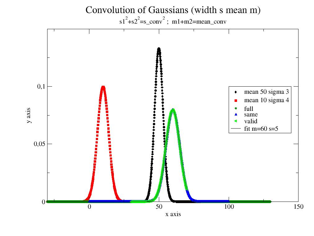
import jscatter as js;import numpy as np

s1=3;s2=4;m1=50;m2=10
G1=js.formel.gauss(np.r_[0:100.1:0.1],mean=m1,sigma=s1)
G2=js.formel.gauss(np.r_[-30:30.1:0.2],mean=m2,sigma=s2)

p=js.grace()
p.title('Convolution of Gaussians (width s mean m)')
p.subtitle(r's1\S2\N+s2\S2\N=s_conv\S2\N ;  m1+m2=mean_conv')
p.plot(G1,le='mean 50 sigma 3')
p.plot(G2,le='mean 10 sigma 4')

ggf=js.formel.convolve(G1,G2,'full')
p.plot(ggf,le='full')

ggs=js.formel.convolve(G1,G2,'same')
p.plot(ggs,le='same')

ggv=js.formel.convolve(G1,G2,'valid')
p.plot(ggv,le='valid')

ggv.fit(js.formel.gauss,{'mean':40,'sigma':1},{},{'x':'X'})
p.plot(ggv.modelValues(),li=1,sy=0,le='fit m=$mean s=$sigma')

p.legend(x=100,y=0.1)
p.xaxis(max=150,label='x axis')
p.yaxis(min=0,max=0.15,label='y axis')
p.save('convolve.jpg')

jscatter.dynamic.cumulant(x, k0=1, k1=0, k2=0, k3=0, k4=0, k5=0)[source]

Cumulant of order ki.

\[I(x) = k_0 exp(-k_1x+1/2k_2x^2-1/6 k_3x^3+1/24k_4x^4-1/120k_5x^5)\]

Cumulants can only be used in initial slope analysis and not for a full fit of DLS data to long times. It is necessary to cut large x. See cumulantDLS() for DLS.

Parameters:

xfloat

Wavevector

k0,k1, k2,k3,k4,k5float

Cumulant coefficients; units 1/x

k0 amplitude

k1 expected value

k2 variance with $\sqrt(k2/k1) =$ relative standard deviation

higher order see Wikipedia

Returns:

dataArray

Examples

import jscatter as js
import numpy as np

t = js.loglist(1e-6,10,1000) # in seconds

p=js.grace()
p.xaxis(scale='log')

k1=1/0.001
for f in [0,0.1,10.5]:
   cum=js.dynamic.cumulant(t,k1=k1,k2=f*2*k1)
   p.plot(cum,sy=0,li=-1)

jscatter.dynamic.cumulantDLS(t, A, G, sigma, skewness=0, bgr=0.0, g2=True)[source]

Cumulant analysis for dynamic light scattering (DLS) or NSE assuming Gaussian size distribution.

See Frisken et al [1] :

\[g_1(t) = A exp(-t/G) \big( 1+(sigma/G t)^2/2. - (skewness/G t)^3/6. \big) + bgr\]

Returns $g_1^2=g_2-1$ for DLS or $g_1(t)$ for NSE.

Parameters:

tarray

Time

Afloat

Amplitude at t=0; Intercept

Gfloat

Mean relaxation time as 1/decay rate in units of t.

sigmafloat

relative standard deviation if a gaussian distribution is assumed
should be smaller 1 or the Taylor expansion is not valid
k2=variance=sigma**2/G**2

skewnessfloat,default 0

Relative skewness k3=skewness**3/G**3

bgrfloat; default 0

Constant background

g2bool default = True

Determines correlation type as field correlation (actually $g_1^2=g_2-1$) or intensity correlation $g_1$.

True is intensity correlations $g_1^2=g_2-1$.

Actually fitting the measured data is prefered, use this for DLS. This should be used for DLS as $g_1^2(t \rightarrow \infty)$ fluctuates around 0 allowing negative values and prevents a bias during fitting.
False is field correlations $g_1$.

Use this e.g. for NSE as the field correlation is measured directly.

Returns:

dataArray

Notes

To fit diffusion constant D e.g. use

def cDLS(t, A, D, sigma, q, bgr=0.0, g2=1):
   # g2=1 or 0 switches between g1 or g2minus1
   # diffusion coefficient in nm*nm/ns  if q in 1/nm and t in microseconds
   G=1/(D*q**2*1000)
   return js.dynamic.cumulantDLS(t=t, A=A, G=G, sigma=sigma, skewness=0, bgr=bgr, g2=True if g2!=0 else False)

References

[1]

Revisiting the method of cumulants for the analysis of dynamic light-scattering data Barbara J. Frisken APPLIED OPTICS 40, 4087 (2001)

Examples

import jscatter as js
import numpy as np

# simulate data
t=js.loglist(0.125,10000,1000)   #times in microseconds
q=4*np.pi*1.333/632*np.sin(np.deg2rad(90)/2) # 90 degrees for 632 nm , unit is 1/nm**2
D=0.01  # nm**2/ns * 1000 = units nm**2/microseconds
noise=0.001  # typical < 1e-3
G = 1/q**2*D
g1 = 0.9*np.exp(-t/G)    # with 20x larger aggragates
data=js.dA(np.c_[t,g1**2 + noise*np.random.randn(len(t))].T)  # intensity correlation with noise

data.makeErrPlot(xscale='log')
data.fit(js.dynamic.cumulantDLS,{'A':0.9, 'G':20, 'sigma':0,'bgr':0},{},{'t':'X'},condition=lambda a:a.Y>0.1)

jscatter.dynamic.diffusionHarmonicPotential(t, q, rmsd, tau, beta=0, ndim=3)[source]

ISF corresponding to the standard OU process for diffusion in harmonic potential for dimension 1,2,3.

The intermediate scattering function corresponding to the standard OU process for diffusion in an harmonic potential [1]. It is used for localized translational motion in incoherent neutron scattering [2] as improvement for the diffusion in a sphere model. Atomic motion may be restricted to ndim=1,2,3 dimensions and are isotropic averaged. The correlation is assumed to be exponential decaying.

Parameters:

tarray

Time values in units ns

qfloat

Wavevector in unit 1/nm

rmsdfloat

Root mean square displacement $rmsd=\langle u_x^2 \rangle ^{1/2}$ in potential in units nm. $\langle u_x^2 \rangle ^{1/2}$ is the width of the potential According to [2] 5*u**2=R**2:math:5langle u_x^2 rangle =R^2 compared to the diffusion in a sphere of radius R.

taufloat

Correlation time $\tau_0$ in units ns. Diffusion constant in sphere Ds=u**2/tau

betafloat, default 0

Exponent in correlation function $\rho(t)$.

beta=0 : $\rho(t) = exp(-t/\tau_0)$ normal liquids where memory effects are presumably weak or negligible [2].

0<beta,inf : $\rho(t,beta) = (1+\frac{t}{\beta\tau_0})^{-\beta}$. See [2] equ. 21a. supercooled liquids or polymers, where memory effects may be important correlation functions with slower decay rates should be introduced [2]. See [2] equ. 21b.

ndim1,2,3, default=3

Dimensionality of the diffusion potential.

Returns:

dataArray

Notes

We use equ. 18-20 from [2] and correlation time $\tau_0$ with equal amplitudes $rmsd=\langle u_x^2 \rangle ^{1/2}$ in the dimensions as

3 dim case:

\[I_s(Q,t) = e^{-Q^2\langle u^2_x \rangle (1-\rho(t))}\]

2 dim case:

\[I_s(Q,t) = \frac{\pi^{0.5}}{2} e^{-g^2(t)} \frac{erfi(g(t))}{g(t)} \ with \ g(t) = \sqrt{Q^2\langle u^2_x \rangle (1-\rho(t))}\]

1 dim case:

\[I_s(Q,t) = \frac{\pi^{0.5}}{2} \frac{erf(g(t))}{g(t)} \ with \ g(t) = \sqrt{Q^2\langle u^2_x \rangle (1-\rho(t))}\]

with erf as the error function and erfi is the imaginary error function erf(iz)/i

References

[1]

Quasielastic neutron scattering and relaxation processes in proteins: analytical and simulation-based models G. R. Kneller Phys. ChemChemPhys. ,2005, 7,2641–2655

[2] (1,2,3,4,5,6,7)

Gaussian model for localized translational motion: Application to incoherent neutron scattering F. Volino, J.-C. Perrin and S. Lyonnard, J. Phys. Chem. B 110, 11217–11223 (2006)

Examples

import numpy as np
import jscatter as js
t=np.r_[0.1:6:0.1]
p=js.grace(1,1)
p.plot(js.dynamic.diffusionHarmonicPotential(t,1,2,1,1),le='1D ')
p.plot(js.dynamic.diffusionHarmonicPotential(t,1,2,1,2),le='2D ')
p.plot(js.dynamic.diffusionHarmonicPotential(t,1,2,1,3),le='3D ')
p.legend()
p.yaxis(label='I(Q,t)')
p.xaxis(label='Q / ns')
p.subtitle('Figure 2 of ref Volino J. Phys. Chem. B 110, 11217')
# p.save(js.examples.imagepath+'/diffusionHarmonicPotential_t.jpg', size=(2,2))

jscatter.dynamic.diffusionHarmonicPotential_w(w, q, tau, rmsd, ndim=3, nmax='auto')[source]

Diffusion in a harmonic potential for dimension 1,2,3 (isotropic averaged), dynamic structure factor in w domain.

An approach worked out by Volino et al.[Rfe0805bd4f86-1]_ assuming Gaussian confinement and leads to a more efficient formulation by replacing the expression for diffusion in a sphere with a simpler expression pertaining to a soft confinement in harmonic potential.

$D_t = \langle u_x^2 \rangle / \tau_0$ see equ. 32 in [1] .

Parameters:

warray: Frequencies in 1/ns
qfloat: Wavevector in nm**-1
taufloat: Mean correlation time $\tau_0$. In units ns.
rmsdfloat: Root mean square displacement $\langle u_x^2 \rangle^{1/2}$ (width) of the Gaussian in units nm.
ndim1,2,3, default=3: Dimensionality of the potential.
nmaxint,’auto’: Order of expansion. ‘auto’ -> nmax = min(max(int(6*q * q * u2),30),1000)

Returns:

dataArray

Notes

Volino et al.[Rfe0805bd4f86-1]_ compared the behavior of this approach to the well known expression for diffusion in a sphere. Even if the details differ, the salient features of both models match if the radius R**2 ≃ 5*u0**2 and the diffusion constant inside the sphere relates to the relaxation time of particle correlation t0= ⟨u**2⟩/Ds towards the Gaussian with width u0=⟨u**2⟩**0.5.

\[I_s(Q_x,\omega) = A_0(Q) + \sum_n^{\infty} A_n(Q) L_n(\omega) \; with \; L_n(\omega) = \frac{\tau_0 n}{\pi (n^2+ \omega^2\tau_0^2)}\]

ndim=3: Here we use the Fourier transform of equ 23 with equ. 27a+b in [1]. For order n>30 the Stirling approximation for n! in equ 27b of [1] is used.

\[A_0(Q) = e^{-Q^2\langle u^2_x \rangle}\]

\[A_n(Q,\omega) = e^{-Q^2\langle u^2_x \rangle} \frac{(Q^2\langle u^2_x \rangle)^n}{n!}\]
ndim=2: Here we use the Fourier transform of equ 23 with equ. 28a+b in [1].

\[A_0(Q) = \frac{\sqrt{\pi} e^{-Q^2\langle u^2_x \rangle}}{2} \frac{erfi(\sqrt{Q^2\langle u^2_x \rangle})}{\sqrt{Q^2\langle u^2_x \rangle}}\]

\[A_n(Q,\omega) = \frac{\sqrt{\pi} (Q^2\langle u^2_x \rangle)^n}{2} \frac{F_{1,1}(1+n;3/2+n;-Q^2\langle u^2_x \rangle)}{\Gamma(3/2+n)}\]

with $F_{1,1}(a,b,z)$ Kummer confluent hypergeometric function, Gamma function $\Gamma$ and erfi is the imaginary error function erf(iz)/i

ndim=1

The equation given by Volino (29a+b in [1]) seems to be wrong as a comparison with the Fourier transform and the other dimensions shows. Use the model from time domain and use FFT as shown in the example.

For experts: To test this remove a flag in the source code and compare.

References

[1] (1,2,3,4,5)

Gaussian model for localized translational motion: Application to incoherent neutron scattering. Volino, F., Perrin, J. C. & Lyonnard, S. J. Phys. Chem. B 110, 11217–11223 (2006).

Examples

import jscatter as js
import numpy as np
t2f = js.dynamic.time2frequencyFF
dHP = js.dynamic.diffusionHarmonicPotential
w = np.r_[-100:100]
ql = np.r_[1,3,6,9,12,15]
iqt3 = js.dL([js.dynamic.diffusionHarmonicPotential_w(w=w,q=q,tau=0.14,rmsd=0.34,ndim=3) for q in ql])
iqt2 = js.dL([js.dynamic.diffusionHarmonicPotential_w(w=w,q=q,tau=0.14,rmsd=0.34,ndim=2) for q in ql])
# as ndim=1 is a wrong solution use this instead
# To move spectral leakage out of our window we increase w and interpolate.
# The needed factor (here 23) depends on the quality of your data and background contribution.
# You may test it using ndim=2 in this example.
iqt1 = js.dL([t2f(dHP,'elastic',w=w*23,q=q, rmsd=0.34, tau=0.14 ,ndim=1).interpolate(w) for q in ql])

p=js.grace(1,1)
p.multi(2,3)
p[1].title('diffusionHarmonicPotential for ndim= 1,2,3')
for i,(i3,i2,i1) in enumerate(zip(iqt3,iqt2,iqt1)):
    p[i].plot(i3,li=1,sy=0,le='$wavevector nm\S-1')
    p[i].plot(i2,li=2,sy=0)
    p[i].plot(i1,li=4,sy=0)
    p[i].yaxis(scale='log')
    if i in [1,2,4,5]:p[i].yaxis(ticklabel=0)
    p[i].legend(x=5,y=1, charsize=0.7)
p[0].xaxis(label='')
p[0].yaxis(label=r'S(\xw)')
p[3].yaxis(label=r'S(\xw)')
# p.save(js.examples.imagepath+'/diffusionHarmonicPotential.jpg', size=(2,2))

jscatter.dynamic.diffusionInSphere_w(w, q, D, R)[source]

Diffusion inside of a sphere; dynamic structure factor in w domain.

Parameters:

warray: Frequencies in 1/ns
qfloat: Wavevector in nm**-1
Dfloat: Diffusion coefficient in units nm**2/ns
Rfloat: Radius of the sphere in units nm.

Returns:

dataArray

Notes

Here we use equ. 33 in [1]

\[S(q,\omega) = A_0^0(q) \delta(\omega) + \frac{1}{\pi} \sum_{l,n\ne 0,0}(2l+1)A_n^l(q) \frac{(x_n^l)^2D/a^2}{[(x_n^l)^2D/a^2]^2 + \omega^2}\]

with $x_n^l$ as the first 99 solutions of equ 27 a+b as given in [1] and

\[A_0^0(q) = \big[ \frac{3j_1(qa)}{qa} \big]^2 , \; (l,n) = (0,0)\]

\[ \begin{align}\begin{aligned}A_n^l(q) &= \frac{6(x_n^l)^2}{(x_n^l)^2-l(l+1)} \big[\frac{qaj_{l+1}(qa)-lj_l(qa)}{(qa)^2-(x_n^l)^2}\big]^2 \; for \; qa\ne x_n^l\\&= \frac{3}{2}j_l^2(x_n^l) \frac{(x_n^l)^2-l(l+1)}{(x_n^l)^2} \; for \; qa = x_n^l\end{aligned}\end{align} \]

This is valid for qR<20 with accuracy of ~0.001 as given in [1]. If we look at a comparison with free diffusion the valid range seems to be smaller.

A comparison of diffusion in different restricted geometry is show in example A comparison of different dynamic models in frequency domain.

References

[1] (1,2,3)

Neutron incoherent scattering law for diffusion in a potential of spherical symmetry: general formalism and application to diffusion inside a sphere. Volino, F. & Dianoux, A. J., Mol. Phys. 41, 271–279 (1980). https://doi.org/10.1080/00268978000102761

Examples

import jscatter as js
import numpy as np
w=np.r_[-100:100]
ql=np.r_[1:14.1:1.3]
p=js.grace(1,1)
iqw=js.dL([js.dynamic.diffusionInSphere_w(w=w,q=q,D=0.14,R=0.2) for q in ql])
p.plot(iqw)
p.yaxis(label=r'S(\xw)',scale='l')
p.xaxis(label=r'\xw\f{} / ns\S-1')
# p.save(js.examples.imagepath+'/diffusionInSphere_w.jpg', size=(2,2))

jscatter.dynamic.diffusionPeriodicPotential(t, q, u, rt, Dg, gamma=1)[source]

Fractional diffusion of a particle in a periodic potential.

The diffusion describes a fast dynamics inside of the potential trap with a mean square displacement before a jump and a fractional long time diffusion. For fractional coefficient gamma=1 normal diffusion is recovered.

Parameters:

tarray: Time points, units ns.
qfloat: Wavevector, units 1/nm
ufloat: Root mean square displacement in the trap, units nm.
rtfloat: Relaxation time of fast dynamics in the trap; units ns ( = 1/lambda in [1] )
gammafloat: Fractional exponent gamma=1 is normal diffusion
Dgfloat: Long time fractional diffusion coefficient; units nm**2/ns.

Returns:

dataArray: [t, Iqt , Iqt_diff, Iqt_trap]

Notes

We use equ. 4 of [1] for fractional diffusion coefficient $D_{\gamma}$ with fraction $\gamma$ as

\[I(Q,t) = exp(-\frac{1}{6}Q^2 msd(t))\]

\[msd(t) = \langle (x(t)-x(0))^2 \rangle = 6\Gamma^{-1}(\gamma+1)D_{\gamma}t^{\gamma} + 6\langle u^2 \rangle (1-E_{\gamma}(-(\lambda t)^{\gamma}))\]

with the Mittag Leffler function $E_{\gamma}(-at^{\gamma})$ and Gamma function $\Gamma$ and $\lambda =1/r_t$.

The first term in msd describes the long time fractional diffusion while the second describes the additional mean-square displacement inside the trap :math:`langle u^2 rangle `.

For $\gamma=1 \to E_{\gamma}(-at^{\gamma}) \to exp(-at)$ simplifying the equation to normal diffusion with traps.

References

[1] (1,2,3)

Gupta, S.; Biehl, R.; Sill, C.; Allgaier, J.; Sharp, M.; Ohl, M.; Richter, D. Macromolecules 49 (5), 1941 (2016). https://doi.org/10.1021/acs.macromol.5b02281

Examples

Example similar to protein diffusion in a mesh of high molecular weight PEG as found in [1].

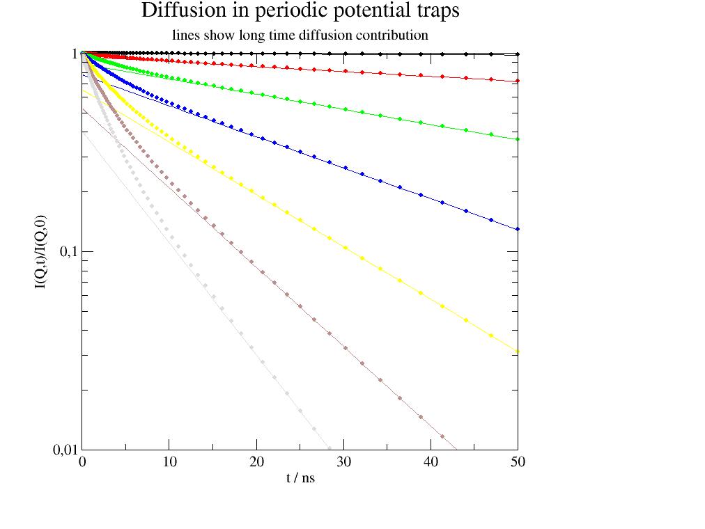
import jscatter as js
import numpy as np
t=js.loglist(0.1,50,100)
p=js.grace()
for i,q in enumerate(np.r_[0.1:2:0.3],1):
    iq=js.dynamic.diffusionPeriodicPotential(t,q,0.5,5,0.036)
    p.plot(iq,symbol=[1,0.3,i],legend='q=$wavevector')
    p.plot(iq.X,iq._Iqt_diff,sy=0,li=[1,0.5,i])
p.title('Diffusion in periodic potential traps')
p.subtitle('lines show long time diffusion contribution')
p.yaxis(max=1,min=1e-2,scale='log',label='I(Q,t)/I(Q,0)')
p.xaxis(min=0,max=50,label='t / ns')
p.legend(x=110,y=0.8)
# p.save(js.examples.imagepath+'/fractalDiff.jpg')

$fractalDiff$

jscatter.dynamic.doubleDiffusion(t, q=None, gamma1=None, D1=None, s1=0, gamma2=None, D2=None, s2=0, frac=0.5, beta=1, type='lognorm')[source]

Intermediate scattering function [g1(t)] for diffusing particles from bimodal distribution of relaxation rates.

\[I_i(q,t,D_i,\sigma_i ) = \int g(\Gamma_i, \Gamma_{i,0} \sigma_i ) e^{-\Gamma_i t} d\Gamma_i\]

\[I(q,t) = beta [f\ I_1(q,t,D_1,\sigma_1 ) + (1-f)\ I_2(q,t,D_2,\sigma_2 )]\]

and relaxation rates $\Gamma_{i,0}=q^2D_i$.

Parameters:

tfloat, array

Times

gamma1,gamma2float

Mean relaxation rates in inverse t units. Overrides q and D if given. If q and D given gamma=q*q*D

qfloat, array

Wavevector

betafloat

Intercept $\beta$ in DLS. The amplitude prefactor.

D1,D2float

Mean diffusion coefficients.

s1,s2float

Relative standard deviations of the diffusion coefficient distributions. In absolute units $\sigma=s*q^2*D$. For a typical DLS experiment s≈0.25 just from instrument noise (e.g. noise ≈ 1e-3 Zetasizer Nano, Malvern)

fracfloat

Fraction of contribution 1. Contribution 2 is (1-frac)

type‘truncnorm’, default ‘lognorm’

Distribution shape.

‘lognorm’ lognorm distribution as normal distribution on a log scale.

\[g(x, \mu, \sigma) = \frac{ 1 }{\ x\sigma\sqrt{2\pi}} exp(-\frac{\ln(x- \mu)^2}{ 2 \sigma^2 })\]

‘truncnorm’ normal distribution cut at zero.

\[g(x, \mu, \sigma)= e^{-0.5(\frac{x-\mu}{\sigma})^2} / (\sigma\sqrt{2\pi}) \ \text{ for x>0}\]

Returns:

outdataArray

Intermediate scattering function or $g_1$

.D1, .D2, .wavevector, .beta respective input parameters

pdf1, pdf2 : Probability of the distribution in the interval around pdf[0,i] (half distance to neighboring points) that sum(pdf[2])==1 similar to CONTIN results.

Notes

Units of q, t and D result in unit-less [q*q*D*t] like q in 1/cm, t in s -> D in cm*cm/s .

Examples

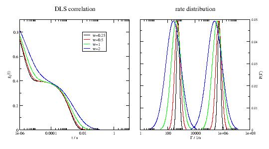
import jscatter as js
import numpy as np

t = js.loglist(1e-6,10,1000) # in seconds
# ≈ a protein with a MW of 140kDa
D1 = 3e-8  # unit cm^2/s
D2 = 3e-5  # unit cm^2/s
q = 4*np.pi/633e-7*np.sin(np.pi/4)  # 90º HeNe laser in DLS

p=js.grace(1.8,1)
p.multi(1,2)
p[0].xaxis(label=r't / s ',scale='log')
p[0].yaxis(label=r'g\s1\N(t) ')
p[1].xaxis(label=r'\xG\f{} / 1/s ',scale='log')
p[1].yaxis(label=[r'P(\xG\f{})',1,'opposite'],)

for c,s in enumerate([0.25,0.5,1,2],1):
   dls = js.dynamic.doubleDiffusion(t=t,q=q,D1=D1,s1=s,D2=D2,s2=s,frac=0.4)
   p[0].plot(dls,sy=0,li=[1,3,c],le=f's={s}')
   p[1].plot(dls.pdf1[0], 20 * dls.pdf1[1],sy=0,li=[1,3,c])
   p[1].plot(dls.pdf2[0], 20 * dls.pdf2[1],sy=0,li=[1,3,c])

p[0].legend(x=0.01,y=0.8)
p[0].title('DLS correlation')
p[1].title('rate distribution')
# p.save(js.examples.imagepath+'/doubleDiffusion.jpg',size=(1.8,1))

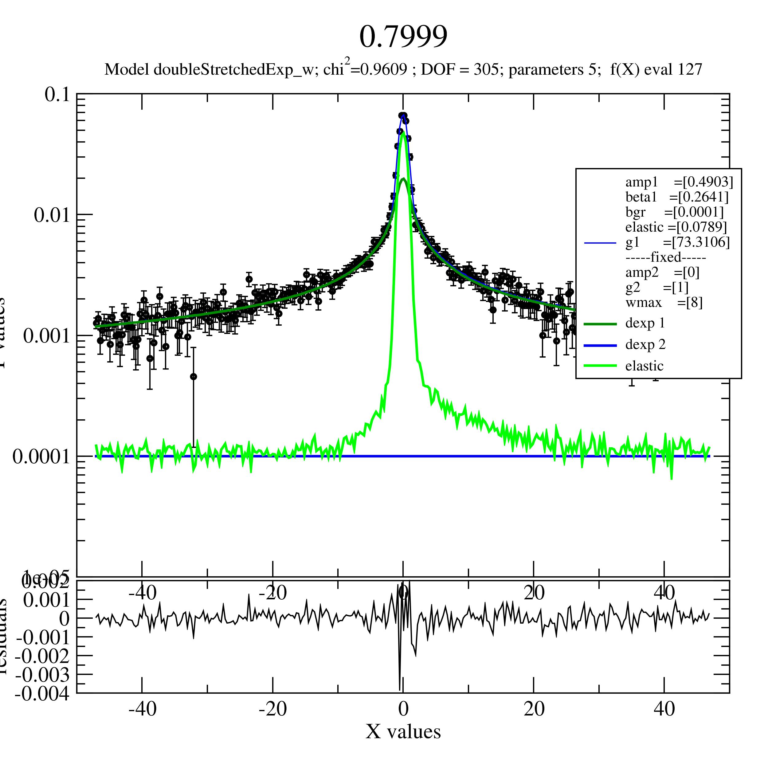
jscatter.dynamic.doubleStretchedExp_w(w, Q, g1, beta1, amp1, resolution, g2=1, beta2=1, amp2=0, elastic=0, bgr=0, wmax=None)[source]

Two stretched exponential with elastic contribution and resolution smearing.

A convenience function that allows to directly fit experimental data.

Remember that fixing beta can mimic different model like beta=1 is Lorentz function, beta = 0.5 fits to subdiffusive Rouse like motions. Each stretchedExp is normalized $\int_{-\infty}^{\infty} \phi(\omega) = 1$

Parameters:

warray

Frequencies 1/ns

Qfloat

Wavevector in 1/nm for selecting the correct resolution.

g1,g2float

Relaxation rates in units 1/[unit t]

beta1,beta2float

Stretched exponent corresponding to g1,g2

amp1,amp2float

Amplitudes of the FF transformed double Exp.

elasticfloat

Amplitude elastic contribution. If the resolution is normalized it is directly the elastic contribution.

resolutiondataList

Measured or calculated resolution function with same Q as in the data to fit.

Normalize the resolution before usage that the elastic amplitude a0 gets meaningful.
In general it is assumed that the resolution and data w are equidistant.
A fitted resolution can be used to smooth noise in a measured resolution. See resolution_w() how to fit and use the ‘.lastfit’ .

bgrfloat

Background.

wmaxfloat, default None

Cutoff frequency for resolution. Not needed for fitted resolution.

Notes

We sum here two stretched exponentials with amplitudes and add an elastic contribution.

For stretched exp see stretchedExp_w() that are convoluted with the resolution cut at wmax.

As elastic contribution we use the measured resolution cut at wmax and multiplied by amplitude elastic

A constant bgr is added.

Examples

import jscatter as js
import numpy as np

def readEMUdat(filename, wavelength=6.27084, temperature=0):
    # Read data form EMU@ANSTO as direct output from Mantid (No .inx converison needed)
    data = js.dL(filename, delimiter=',')
    for da in data:
        da.Q = np.round(float(da.comment[0]),4)
        da.temperature = temperature
        da.wavelength = wavelength
    # cut the zero at the end 
    for i in range(len(data)):
        data[i] = data[i,:,:-1]
    return data

resoe = readEMUdat(js.examples.datapath + '/sample_5K_Q.dat.gz', temperature=5)
reso = js.dynamic.convert_e2w(resoe, 0, unit='meV')
# convert resolution to normalized data that elastic has meaning
for va in reso:
    va.Y = va.Y/np.trapezoid(va.Y,va.X)  # normalize resolution

# read new data and convert to 1/ns
same = readEMUdat(js.examples.datapath + '/sample_413K_Q.dat.gz',temperature=413)
sam = js.dynamic.convert_e2w(same, 293, unit='meV')

# Fit one after the other
for n in np.r_[0:len(sam)]:
    #sam[n].makeErrPlot(yscale='log', title=str(sam[n].Q) + ' A\S-1')
    sam[n].setlimit()  # removes limits
    sam[n].setlimit(elastic=[0, 1], bgr=[0.0001, 0.01])  # bgr lower bound arbitrary, should be >0
    sam[n].setlimit(ampl=[0,10],amp2=[0])                # no negative amplitudes
    sam[n].setlimit(g1=[0,100],g2=[0,100])               # no negative and some max fwhm
    sam[n].setlimit(beta1=[0,1],beta2=[0,1])             # no negative and some max fwhm
    sam[n].fit(js.dynamic.doubleStretchedExp_w,
        {'elastic': 1, 'bgr': 2e-4, 'amp1': 0.2,'g1':16, 'beta1':1},
        {'wmax':8, 'amp2':0,'g2': 1,'resolution':reso},
        {'w': 'X'},
        method='lm',max_nfev=20000)
    #sam[n].killErrPlot()  # close it , or uncomment to have them open

# look at one single errplot
n=3
sam[n].showlastErrPlot(title=str(sam[n].Q) , yscale='log')
sam[n].errPlot(sam[n].lastfit.X,sam[n].lastfit._se1,sy=0,li=[1,2,3],le='dexp 1')  # add
sam[n].errPlot(sam[n].lastfit.X,sam[n].lastfit._se2,sy=0,li=[1,2,4],le='dexp 2')
sam[n].errPlot(sam[n].lastfit.X,sam[n].lastfit._el,sy=0,li=[1,2,5],le='elastic')

# sam[n].errplot.save(js.examples.imagepath+'/doubleStretchedExp_w.jpg', size=(2,2))

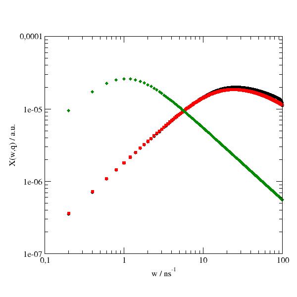
jscatter.dynamic.dynamicSusceptibility(data, Temp)[source]

Transform from S(w,q) to the imaginary part of the dynamic susceptibility.

\[ \begin{align}\begin{aligned}\chi (w,q) &= \frac{S(w,q)}{n(w)} (gain side)\\ &= \frac{S(w,q)}{n(w)+1} (loss side)\end{aligned}\end{align} \]

with Bose distribution for integer spin particles

\[with \ n(w)=\frac{1}{e^{hw/kT}-1}\]

Parameters:

datadataArray: Data to transform with w units in 1/ns
Tempfloat: Measurement temperature in K.

Returns:

dataArray

Notes

“Whereas relaxation processes on different time scales are usually hard to identify in S(w,q), they appear as distinct peaks in dynamic susceptibility with associated relaxation times $\tau ~(2\pi\omega)^{-1}$ [1].

References

[1]

Roh et al. ,Biophys. J. 91, 2573 (2006), doi: 10.1529/biophysj.106.082214

Examples

#
import jscatter as js
import numpy as np
start={'s0':5,'m0':0,'a0':1,'bgr':0.00}
w=np.r_[-100:100:0.2]
resolution=js.dynamic.resolution_w(w,**start)

# model
def diffindiffSphere(w,q,R,Dp,Ds,w0,bgr):
    diff_w=js.dynamic.transDiff_w(w,q,Ds)
    rot_w=js.dynamic.diffusionInSphere_w(w=w,q=q,D=Dp,R=R)
    Sx=js.formel.convolve(rot_w,diff_w)
    Sxsb=js.dynamic.shiftAndBinning(Sx,w=w,w0=w0)
    Sxsb.Y+=bgr       # add background
    return Sxsb

q=5.5;R=0.5;Dp=1;Ds=0.035;w0=1;bgr=1e-4
Iqw=diffindiffSphere(w,q,R,Dp,Ds,w0,bgr)
IqwR=js.dynamic.diffusionInSphere_w(w,q,Dp,R)
IqwT=js.dynamic.transDiff_w(w,q,Ds)
Xqw=js.dynamic.dynamicSusceptibility(Iqw,293)
XqwR=js.dynamic.dynamicSusceptibility(IqwR,293)
XqwT=js.dynamic.dynamicSusceptibility(IqwT,293)
p=js.grace()
p.plot(Xqw)
p.plot(XqwR)
p.plot(XqwT)
p.yaxis(scale='l',label='X(w,q) / a.u.',min=1e-7,max=1e-4)
p.xaxis(scale='l',label='w / ns\S-1',min=0.1,max=100)
# p.save(js.examples.imagepath+'/susceptibility.jpg', size=(2,2))

jscatter.dynamic.elastic_w(w)[source]

Elastic line; dynamic structure factor in w domain.

$\delta(w)$ distribution at I(w)=0 except I(0)=a that np.trapezoid(I(w)) =1

Parameters:

warray: Frequencies in 1/ns. Zero value should be part of w.

Returns:

dataArray

Notes

For shifted frequencies (e.g. to be symmetric around zero) the elastic peak position (zero value) might not appear on the X values.

jscatter.dynamic.finiteRouse(t, q, NN=None, pmax=None, l=None, frict=None, Dcm=None, Wl4=None, Dcmfkt=None, tintern=0.0, Temp=293, ftype=None, specm=None, specb=None, rk=None)[source]

Rouse dynamics of a finite chain with N beads of bonds length l and internal friction.

The Rouse model describes the conformational dynamics of an ideal chain. The single chain diffusion is represented by Brownian motion of beads connected by harmonic springs. No excluded volume, random thermal force, drag force with solvent, no hydrodynamic interaction and optional internal friction. Coherent + incoherent scattering.

Parameters:

tarray

Time in units nanoseconds

qfloat, list

Scattering vector, units nm^-1 For a list a dataList is returned otherwise a dataArray is returned

NNinteger

Number of chain beads.

lfloat, default 1

Bond length between beads; unit nm.

pmaxinteger, list of floats

integer => maximum mode number ($a_p=1$)
list => $a_p$ list of amplitudes>0 for individual modes to allow weighing; not given modes have weight zero

frictfloat

Friction of a single bead/monomer in units Pas*m=kg/s=1e-6 g/ns $\xi = 6\pi\eta l$, . A monomer bead with l=R=0.1nm = 0.1e-9m in H2O(20°C) (1 mPas) => 1.89e-12 Pas*m. Rouse dynamics in a melt needs the bead friction with effective viscosity of the melt.

Wl4float

$W_l^4$ Characteristic value to calc friction and Dcm.

$D_{cm}=\frac{W_l^4}{3R_e^2}$ and characteristic Rouse variable $\Omega_Rt=(q^2/6)^2 W_l^4 t$

Dcmfloat

Center of mass diffusion in nm^2/ns.

$D_{cm}=k_bT/(N\xi)$ with $\xi$ = friction of single bead in solvent
$D_{cm}=W_l^4/(3Nl^2)=W_l^4/(3Re^2)$

Dcmfktarray 2xN, function

Function f(q) or array with [qi, f(qi) ] as correction for Dcm like Diff = Dcm*f(q). e.g. for inclusion of structure factor or hydrodynamic function with f(q)=H(Q)/S(q). Missing values are interpolated.

tinternfloat>0

Relaxation time due to internal friction between neighboring beads in ns.

ftype‘rni’, ‘rap’,’nonspec’, ‘specrif’, ‘crif’, default = ‘rif’

Type of internal friction. See [7] for a description and respective references.

‘rif’: Internal friction between neighboring beads in chain. $t_{rp}=t_r p^{-2}+t_{intern}$
‘rni’: Rouse model with non-local interactions (RNI). Additional friction between random close approaching beads. $t_{rp}=t_r p^{-2}+N/p t_{intern}$
‘rap’: Rouse model with anharmonic potentials due to stiffness of the chain $t_{rp}=t_r p^{-2}+t_{intern}ln(N/p\pi)$
‘specrif’: Specific interactions of strength $b$ between beads separated by m bonds. See [7]. $t_{rp}=t_r p^{-2} (1+bm^2)^{-1} + (1+m^2/(1+bm^2))t_{intern}$
‘crif’: Bead confining potential with internal friction. The beads are confined in an additional harmonic potential with $\frac{1}{2}k_c(r_n-0)^2$ leading to a more compact configuration. $rk= k_c/k$ describes the relative strength compared to the force between beads $k$.

Tempfloat

Temperature Kelvin = 273+T[°C]

specm,specb: float

Parameters m, b used in internal friction models ‘spec’ and ‘specrif’.

rkNone , float

$rk= k_c/k$ describes the relative force constant for ftype ‘crif’.

Returns:

S(q,t)/S(q,0)dataArrayfor single q, dataListmultiple q

[time; Sqt; Sqt_inf; Sqtinc]
time units ns
Sqt is S(q,t)/S(q,0) coherent scattering with diffusion and mode contributions
Sqt_inf is coherent scattering with ONLY diffusion
Sqtinc is incoherent scattering with diffusion and mode contributions (no separate diffusion)
.q wavevector
.Iq normalized form factor
.Wl4
.Re end to end distance $R_e^2=l^2N$
.trouse rotational correlation time or rouse time
$tr_1 = \xi N^2 l^2/(3 \pi^2 k_bT)= <R_e^2>/(3\pi D_{cm}) = N^2\xi/(pi^2k)$
.tintern relaxation time due to internal friction
.tr_p characteristic times $tr_p=tr_1 p^{-2}+t_{intern}$
.beadfriction
.ftype type of internal friction
…. use .attr to see all attributes

Notes

The Rouse model describes beads connected by harmonic springs without hydrodynamic interactions and open ends. The coherent intermediate scattering function $S(q,t)$ is [1] [2] :

\[S(q,t) = \frac{1}{N} e^{-q^2D_{cm}t} \sum_{n,m}^N e^{-\frac{1}{6}q^2B(n,m,t)}\]

\[B(n,m,t)=|n-m|^{2\nu}l^2 + \sum_{p=1}^{N-1} A_p cos(\pi pn/N)cos(\pi pm/N) (1-e^{-t/t_{rp}})\]

and for incoherent intermediate scattering function the same with $n=m$ in the first sum.

with

$A_p = a_p\frac{4R_e^2}{\pi^2}\frac{1}{p^2}$ mode amplitude (usual $a_p=1$)

$t_{rp} = \frac{t_r}{p^2}$ mode relaxation time with Rouse time $t_r =\frac{\xi N R_e^2 }{3\pi^2 k_bT} = \frac{R_e^2}{3\pi^2 D_{cm}} = \frac{N^2 \xi}{\pi^2 k}$

$D_{cm}=kT/{N\xi}$ center of mass diffusion

$k=3k_bT/l^2$ force constant k between beads.

$\xi=6\pi visc R$ single bead friction $\xi$ in solvent (e.g. surrounding melt)

$t_{intern}=\xi_i/k$ additional relaxation time due to internal friction $\xi_i$

Modifications (ftype) for internal friction and additional interaction (see [7] and [9]):

RIF : Rouse with internal friction between neighboring beads in chain [3] [4].
- $t_{rp}=t_r p^{-2}+t_{intern}$
- $\xi_i=t_{intern}k=t_{intern}3k_bT/l^2$ internal friction per bead
RNI : Rouse model with non-local interactions as additional friction between spatial close beads [5] .
- $t_{rp}=t_r p^{-2}+Nt_{intern}/p$
RAP : Rouse model with anharmonic potentials in bonds describing the stiffness of the chain [6].
- $t_{rp}=t_r p^{-2}+t_{intern}ln(N/p\pi)$
SPECRIF : Specific interactions of relative strength $b$ between beads separated by m bonds.
Internal friction between neighboring beads as in RIF is added.
- $t_{rp}=t_r p^{-2} (1+bm^2)^{-1} + (1+\frac{m^2}{1+bm^2})t_{intern}$
- $b=k_{specific}/k_{neighbor}$ relative strength of both interactions.
- The interaction is between all pairs separated by m.
CRIF : Compacted Rouse with internal friction [9].
The beads are confined in an additional harmonic potential with $\frac{1}{2}k_c(r_n-0)^2$ leading to a more compact configuration. $rk= k_c/k$ describes the relative strength compared to the force between beads $k$. Typically $rk << 1$ .
- The mode amplitude prefactor changes from Rouse type to modified confined amplitudes
  
  \[A_p =\frac{4R_e^2}{\pi^2}\frac{1}{p^2}\Rightarrow A_p^c = \frac{4R_e^2}{\pi^2}\frac{1}{\frac{N^2k_c}{\pi^2k}+p^2}\]
- The mode relaxation time changes from Rouse type to modified confined
  
  \[t_{rp} = \frac{t_r}{p^2} \Rightarrow t_{rp}^c = \frac{t_r}{\frac{N^2k_c}{\pi^2k} + p^2}\]
- $R_e$ allows to determine $k_c/k$ from small angle scattering data
  
  \[R_e^2 = \frac{2l^2}{\sqrt{k_c/k}}tanh(\frac{N}{2}\sqrt{k_c/k})\]
- We assume here that the additional potential is $\frac{1}{2}k_c(r_n-r_0)^2$ with $r_0$ as the polymer center of mass. As the Langevin equation only depends on relative distances the internal motions are not affected. The center of mass diffusion $D_{cm}=f(R_e)$ is not affected as the mode dependent friction coefficients don’t change [9].
- With $rk=k_c/k \rightarrow 0$ the original Rouse is recovered for amplitudes, relaxation and $R_e$ .

A combination of different effects is possible [7] (but not implemented).

The amplitude $A_p$ allows for additional suppression of specific modes e.g. by topological constraints (see [8]).

From above the triple Dcm,l,NN are fixed.

If 2 are given 3rd is calculated

If all 3 are given the given values are used

For an example see example_Zimm and Zimm dynamics including collective effects (H(Q)/S(Q)) on center of mass diffusion how to include collective effects.

References

[1]

Doi Edwards Theory of Polymer dynamics in the appendix the equation is found

[2]

Nonflexible Coils in Solution: A Neutron Spin-Echo Investigation of Alkyl-Substituted Polynorbonenes in Tetrahydrofuran Michael Monkenbusch et al.Macromolecules 2006, 39, 9473-9479 The exponential is missing a “t” http://dx.doi.org/10.1021/ma0618979

about internal friction

[3]

Exploring the role of internal friction in the dynamics of unfolded proteins using simple polymer models Cheng et al.JOURNAL OF CHEMICAL PHYSICS 138, 074112 (2013) http://dx.doi.org/10.1063/1.4792206

[4]

Rouse Model with Internal Friction: A Coarse Grained Framework for Single Biopolymer Dynamics Khatri, McLeish| Macromolecules 2007, 40, 6770-6777 http://dx.doi.org/10.1021/ma071175x

[5]

Origin of internal viscosities in dilute polymer solutions P. G. de Gennes J. Chem. Phys. 66, 5825 (1977); https://doi.org/10.1063/1.433861

[6]

Microscopic theory of polymer internal viscosity: Mode coupling approximation for the Rouse model. Adelman, S. A., & Freed, K. F. (1977). The Journal of Chemical Physics, 67(4), 1380–1393. https://doi.org/10.1063/1.435011

[7] (1,2,3,4)

Internal friction in an intrinsically disordered protein - Comparing Rouse-like models with experiments A. Soranno, F. Zosel, H. Hofmann J. Chem. Phys. 148, 123326 (2018) http://aip.scitation.org/doi/10.1063/1.5009286

[8]

Onset of topological constraints in polymer melts: A mode analysis by neutron spin echo spectroscopy D. Richter, L. Willner, A. Zirkel, B. Farago, L. J. Fetters, and J. S. Huang Phys. Rev. Lett. 71, 4158 https://doi.org/10.1103/PhysRevLett.71.4158

[9] (1,2,3)

Looping dynamics of a flexible chain with internal friction at different degrees of compactness. Samanta, N., & Chakrabarti, R. (2015). Physica A: Statistical Mechanics and Its Applications, 436, 377–386. https://doi.org/10.1016/j.physa.2015.05.042

Examples

Coherent and incoherent contributions to Rouse dynamics. To mix the individual q dependent contributions have to be weighted with the according formfactor respectivly incoherent scattering length and instrument specific measurement technique.

import jscatter as js
import numpy as np
t = js.loglist(0.02, 100, 40)
q=np.r_[0.1:2:0.2]
l=0.38  # nm , bond length amino acids
rr = js.dynamic.finiteRouse(t, q, 124, 7, l=0.38, Dcm=0.37, tintern=0., Temp=273 + 60)
p=js.grace()
p.multi(2,1)
p[0].xaxis(scale='log')
p[0].yaxis(label='I(q,t)\scoherent')
p[1].xaxis(label=r't / ns',scale='log')
p[1].yaxis(label=r'I(q,t)\sincoherent')
p[0].title('Rouse dynamics in a solvent')
for i, z in enumerate(rr, 1):
    p[0].plot(z.X, z.Y, line=[1, 1, i], symbol=0, legend='q=%g' % z.q)
    p[0].plot(z.X, z._Sqt_inf, line=[3, 2, i], symbol=0, legend='q=%g diff' % z.q)
    p[1].plot(z.X, z._Sqtinc, line=[1, 2, i], symbol=0, legend='q=%g diff' % z.q)

#p.save(js.examples.imagepath+'/Rousecohinc.jpg')

jscatter.dynamic.finiteZimm(t, q, NN=None, pmax=None, l=None, Dcm=None, Dcmfkt=None, tintern=0.0, mu=0.5, viscosity=1.0, ftype=None, rk=None, Temp=293)[source]

Zimm dynamics of a finite chain with N beads with internal friction and hydrodynamic interactions.

The Zimm model describes the conformational dynamics of an ideal chain with hydrodynamic interaction between beads. The single chain diffusion is represented by Brownian motion of beads connected by harmonic springs. Coherent + incoherent scattering.

Parameters:

tarray

Time in units nanoseconds.

q: float, array

Scattering vector in units nm^-1. If q is list a dataList is returned otherwise a dataArray is returned.

NNinteger

Number of chain beads. If not given calculated from Dcm,l, mu.

lfloat, default 1

Bond length between beads; units nm. If not given calculated from Dcm, NN, mu .

pmaxinteger, list of float, default is NN

integer => maximum mode number taken into account.
list => list of amplitudes $a_p > 0$ for individual modes to allow weighing. Not given modes have weight zero.

Dcmfloat

Center of mass diffusion in nm²/ns if explicitly is given. If not given Dcm is calculated

$=0.196 k_bT/(R_e visc)$ for theta solvent with $\nu=0.5$

$=0.203 k_bT/(R_e visc)$ for good solvent with $\nu=0.6$

with $R_e=lN^{\nu}$ .

Dcmfktarray 2xN, function

Function f(q) or array with [qi, f(qi)] as correction for Dcm like Diff = Dcm*f(q). e.g. for inclusion of structure factor and hydrodynamic function with f(q)=H(Q)/S(q). Missing values are interpolated.

tinternfloat>0

Additional relaxation time due to internal friction between neighboring beads in units ns.

mufloat in range [0.01,0.99]

$\nu$ describes solvent quality.

<0.5 collapsed chain
=0.5 theta solvent 0.5 (gaussian chain)
=0.6 good solvent
>0.6 swollen chain

viscosityfloat

$\eta$ in units cPoise=mPa*s

e.g. water $visc(T=293 K) =1 mPas$

Tempfloat, default 273+20

Temperature in Kelvin.

ftype‘czif’, default = ‘zif’

Type of internal friction and interaction modification.

Default Zimm is used with $t_{intern}=0$
‘zif’ Internal friction between neighboring beads in chain [3].

$t_{zp}=t_z p^{-3\nu}+t_{intern}$
‘czif’ Bead confining harmonic potential with internal friction, only for $\nu=0.5$ [6] .

The beads are confined in an additional harmonic potential with $\frac{1}{2}k_c(r_n-0)^2$ leading to a more compact configuration. $rk= k_c/k$ describes the relative strength compared to the force between beads $k$.

rkNone , float

$rk= k_c/k$ describes the relative force constant for ftype ‘czif’.

Returns:

S(q,t)/S(q,0)dataArrayfor single q, dataListfor multiple q

[time; Sqt; Sqt_inf; Sqtinc; Sqtz]
time units ns
Sqt as S(q,t)/S(q,0) coherent scattering with diffusion and mode contributions
Sqt_inf is coherent scattering with ONLY diffusion (no internal modes)
Sqtinc is incoherent scattering with diffusion and mode contributions (no separate diffusion)
Sqtz is coherent scattering with diffusion and mode contributions, but no Dcmfkt => f(q)=1
.q wavevector
.modecontribution $a_p$ of coherent modes i in sequence as in PRL 71, 4158 equ (3)
.Re
.tzimm => Zimm time or rotational correlation time
.t_p characteristic times
…. use .attr for all attributes

Notes

The Zimm model describes beads connected by harmonic springs with hydrodynamic interaction and free ends. The $\nu$ parameter scales between theta solvent $\nu=0.5$ and good solvent $\nu=0.6$ (excluded volume or swollen chain). The coherent intermediate scattering function $S(q,t)$ is

\[S(q,t) = \frac{1}{N} e^{-q^2D_{cm}t}\sum_{n,m}^N e^{-\frac{1}{6}q^2B(n,m,t)}\]

\[B(n,m,t)=|n-m|^{2\nu}l^2 + \sum_{p=1}^{N-1} A_p cos(\pi pn/N)cos(\pi pm/N) (1-e^{-t/t_{zp}})\]

and for incoherent intermediate scattering function the same with $n=m$ in the first sum.

with

$A_p = a_p\frac{4R_e^2}{\pi^2}\frac{1}{p^{2\nu+1}}$ mode amplitude (usual $a_p=1$)
$t_{zp} = t_z p^{-3\nu}$ mode relaxation time
$t_z = \eta R_e^3/(\sqrt(3\pi) k_bT)$ Zimm mode relaxation time
$R_e=l N^{\nu}$ end to end distance
$k=3kT/l^2$ force constant between beads
$\xi=6\pi\eta l$ single bead friction in solvent with viscosity $\eta$
$a_p$ additional amplitude for suppression of specific modes e.g. by topological constraints (see [5]).
$D_{cm} = \frac{8}{3(6\pi^3)^{1/2}} \frac{k_bT}{\eta R_e} = 0.196 \frac{k_bT}{\eta R_e}$

Modifications (ftype) for internal friction and additional interaction:

ZIF : Zimm with internal friction between neighboring beads in chain [3] [4].
- $t_{zp}=t_z p^{{-3\nu}}+t_{intern}$
- $\xi_i=t_{intern}k=t_{intern}3k_bT/l^2$ internal friction per bead
CZIF : Compacted Zimm with internal friction [6].
Restricted to $\nu=0.5$ , a combination with excluded volume is not valid. In [9]_ the beads are confined in an additional harmonic potential around the origin with $\frac{1}{2}k_c(r_n-0)^2$ leading to a more compact configuration. $rk= k_c/k$ describes the relative strength compared to the force between beads $k$. Typically $rk << 1$ .
- The mode amplitude prefactor changes from Zimm type to modified confined amplitudes
  
  \[A_p =\frac{4Nl^2}{\pi^2}\frac{1}{p^2}\Rightarrow A_p^c = \frac{4Nl^2}{\pi^2}\frac{1}{\frac{N^2k_c}{\pi^2k}+p^2}\]
- The mode relaxation time changes from Zimm type to modified confined with $t_{z} = \frac{\eta N^{3/2} l^3}{\sqrt(3\pi) k_bT}$
  
  \[t_{zp} = t_z \frac{1}{p^{3/2}} \Rightarrow t_{zp}^c = t_z \frac{p^{1/2}}{\frac{N^2k_c}{\pi^2k} + p^2}\]
- $R_e^c$ allows to determine $k_c/k$ from small angle scattering data
  
  \[(R_e^c)^2 = \frac{2l^2}{\sqrt{k_c/k}}tanh(\frac{N}{2}\sqrt{k_c/k})\]
- For a free diffusing chain we assume here (not given in [9]_ ) that the additional potential is $\frac{1}{2}k_c(r_n-r_0)^2$ with $r_0$ as the polymer center of mass. As the Langevin equation only depends on position distances the internal motions are not affected. The center of mass diffusion $D_{cm}$ can be calculated similar to the Zimm $D_{cm}$ in [1] assuming a Gaussian configuration with width $R_e$. We find
  
  \[D_{cm} = \frac{kT}{\xi_{p=0}} = \frac{8}{3(6\pi^3)^{1/2}} \frac{kT}{\eta R_e}\]
- With $rk=k_c/k \rightarrow 0$ the original Zimm is recovered for amplitudes, relaxation and $R_e$ .

From above the triple Dcm,l,N are fixed.

If 2 are given 3rd is calculated.

If all 3 are given the given values are used.

For an example see example_Zimm and Zimm dynamics including collective effects (H(Q)/S(Q)) on center of mass diffusion .

References

[1]

Doi Edwards Theory of Polymer dynamics in appendix the equation is found

[2]

Nonflexible Coils in Solution: A Neutron Spin-Echo Investigation of Alkyl-Substituted Polynorbonenes in Tetrahydrofuran Michael Monkenbusch et al.Macromolecules 2006, 39, 9473-9479 The exponential is missing a “t” http://dx.doi.org/10.1021/ma0618979

about internal friction

[3] (1,2)

Exploring the role of internal friction in the dynamics of unfolded proteins using simple polymer models Cheng et al.JOURNAL OF CHEMICAL PHYSICS 138, 074112 (2013) http://dx.doi.org/10.1063/1.4792206

[4]

Rouse Model with Internal Friction: A Coarse Grained Framework for Single Biopolymer Dynamics Khatri, McLeish| Macromolecules 2007, 40, 6770-6777 http://dx.doi.org/10.1021/ma071175x

mode contribution factors from

[5]

Onset of Topological Constraints in Polymer Melts: A Mode Analysis by Neutron Spin Echo Spectroscopy D. Richter et al.PRL 71,4158-4161 (1993)

[6] (1,2)

Looping dynamics of a flexible chain with internal friction at different degrees of compactness. Samanta, N., & Chakrabarti, R. (2015). Physica A: Statistical Mechanics and Its Applications, 436, 377–386. https://doi.org/10.1016/j.physa.2015.05.042

Examples

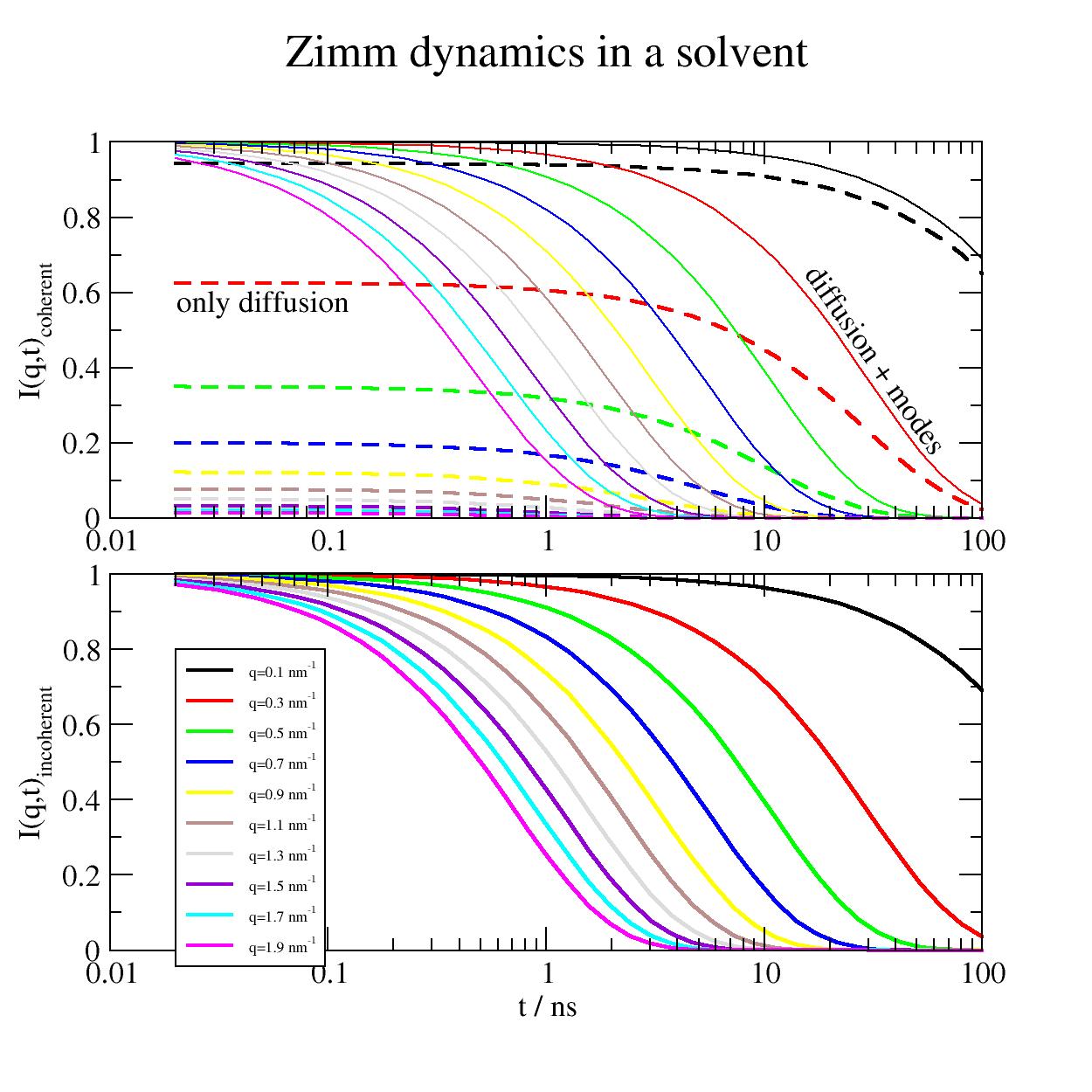
Coherent and incoherent contributions to Zimm dynamics. To mix the individual q dependent contributions of coherent and incoherent these have to be weighted by the according formfactor respectively incoherent scattering length and instrument specific measurement technique. Typically, diffusion and mode contributions cannot be separated. At larger Q the diffusion contributes marginally while at low Q diffusion dominates.

import jscatter as js
import numpy as np
t = js.loglist(0.02, 100, 40)
q=np.r_[0.1:2:0.2]
l=0.38  # nm , bond length amino acids
zz = js.dynamic.finiteZimm(t, q, 124, 7, l=0.38, Dcm=0.37, tintern=0., Temp=273 + 60)
p=js.grace(2,2)
p.multi(2,1)
p[0].xaxis(scale='log')
p[0].yaxis(label='I(q,t)\scoherent')
p[1].xaxis(label=r't / ns',scale='log')
p[1].yaxis(label=r'I(q,t)\sincoherent')
p[0].title('Zimm dynamics in a solvent')
for i, z in enumerate(zz, 1):
    p[0].plot(z.X, z.Y, line=[1, 1, i], symbol=0, legend='')
    p[0].plot(z.X, z._Sqt_inf, line=[3, 2, i], symbol=0, legend='')
    p[1].plot(z.X, z._Sqtinc, line=[1, 2, i], symbol=0, legend=fr'q={z.q:.1f} nm\S-1')
p[1].legend(x=0.02,y=0.8,charsize=0.5)
p[0].text('only diffusion', x=0.02,y=0.55)
p[0].text('diffusion + modes', x=15,y=0.65,rot=305)

# p.save(js.examples.imagepath+'/Zimmcohinc.jpg',size=(1,1))

jscatter.dynamic.fixedFiniteRouse(t, q, NN=None, pmax=None, l=None, frict=None, Dcm=None, Wl4=None, Dcmfkt=None, tintern=0.0, Temp=293, ftype=None, specm=None, specb=None, rk=None, fixedends=1)[source]

Rouse dynamics of a chain with fixed ends with N beads of bonds length l and internal friction.

Opposite to the finiteRouse() here one or both ends are fixed. This might be a chain tethered to a particle that defines the diffusion. Chains are non interacting.

Parameters:

fixedends0,1,2, default = 1

Number of fixed ends. 0 is only for comparison and corresponds to finiteZimm() .

tarray

Time in units nanoseconds

qfloat, list

Scattering vector, units nm^-1 For a list a dataList is returned otherwise a dataArray is returned

NNinteger

Number of chain beads.

lfloat, default 1

Bond length between beads; unit nm.

pmaxinteger, list of floats

integer => maximum mode number ($a_p=1$)
list => $a_p$ list of amplitudes>0 for individual modes to allow weighing; not given modes have weight zero

frictfloat

Friction of a single bead/monomer in units Pas*m=kg/s=1e-6 g/ns$\xi = 6\pi\eta l$, .

A monomer bead with l=R=0.1nm = 0.1e-9m in H2O(20°C) (1 mPas) => 1.89e-12 Pas*m.

Rouse dynamics in a melt needs the bead friction with effective viscosity of the melt which should be much higher than water. Polymer melts are typically examined above the glass temperature of the polymer.

Wl4float

$W_l^4$ Characteristic value to calc friction and Dcm.

$\Omega_Rt=(q^2/6)^2 W_l^4 t$

Dcmfloat

Center of mass diffusion in nm^2/ns.

Dcmfktarray 2xN, function

Function f(q) or array with [qi, f(qi) ] as correction for Dcm like Diff = Dcm*f(q). e.g. for inclusion of structure factor or hydrodynamic function with f(q)=H(Q)/S(q). Missing values are interpolated.

tinternfloat>0

Relaxation time due to internal friction between neighboring beads in ns.

ftype‘rni’, ‘rap’,’nonspec’, ‘specrif’, ‘crif’, default = ‘rif’

Type of internal friction. See [7] for a description and respective references.

‘rif’: Internal friction between neighboring beads in chain. $t_{rp}=t_r p^{-2}+t_{intern}$
‘rni’: Rouse model with non-local interactions (RNI). Additional friction between random close approaching beads. $t_{rp}=t_r p^{-2}+N/p t_{intern}$
‘rap’: Rouse model with anharmonic potentials due to stiffness of the chain $t_{rp}=t_r p^{-2}+t_{intern}ln(N/p\pi)$
‘specrif’: Specific interactions of strength $b$ between beads separated by m bonds. See [7]. $t_{rp}=t_r p^{-2} (1+bm^2)^{-1} + (1+m^2/(1+bm^2))t_{intern}$
‘crif’: Bead confining potential with internal friction. The beads are confined in an additional harmonic potential with $\frac{1}{2}k_c(r_n-0)^2$ leading to a more compact configuration. $rk= k_c/k$ describes the relative strength compared to the force between beads $k$.

Tempfloat

Temperature Kelvin = 273+T[°C]

specm,specb: float

Parameters m, b used in internal friction models ‘spec’ and ‘specrif’.

rkNone , float

$rk= k_c/k$ describes the relative force constant for ftype ‘crif’.

Returns:

S(q,t)/S(q,0)dataArray for single q, dataList for multiple q

[time; Sqt; Sqt_inf; Sqtinc]
time units ns
Sqt is S(q,t)/S(q,0) coherent scattering with diffusion and mode contributions
Sqt_inf is coherent scattering with ONLY diffusion
Sqtinc is incoherent scattering with diffusion and mode contributions (no separate diffusion)
.q wavevector
.Wl4
.Re end to end distance $R_e^2=l^2N$
.trouse rotational correlation time or rouse time
$tr_1 = \xi N^2 l^2/(3 \pi^2 k_bT)= <R_e^2>/(3\pi D_{cm}) = N^2\xi/(pi^2k)$
.tintern relaxation time due to internal friction
.tr_p characteristic times $tr_p=tr_1 p^{-2}+t_{intern}$
.beadfriction
.ftype type of internal friction
…. use .attr to see all attributes

Notes

The Rouse model describes beads connected by harmonic springs without hydrodynamic interactions and open ends. The coherent intermediate scattering function $S(q,t)$ is [1] [2] :

\[S(q,t) = \frac{1}{N} e^{-q^2D_{cm}t} \sum_{n,m}^N e^{-\frac{1}{6}q^2B(n,m,t)}\]

$B(n,m,t)$ describes the internal motions characterised by eigenmodes of the equation 4.II.6 in [1] $\frac{\zeta_p}{\zeta} k \frac{\partial^2 \Phi_{pn}}{\partial^2 n}=-k_p\Phi_{pn}$ where $\Phi_{pn}$ describes the delocalisation of bead n in mode p.

The boundary conditions select the eigenmodes from the general form $\Phi_{pn} = A sin(kn) + Bcos(kn)$

Two free ends $\partial\Phi_{pn}/\partial n=0 \text{ for n=0 and n=N}$ select A=0 and k=pπ/N (equ. 4.II.7+9 in [1]):

\[B(n,m,t)=|n-m|^{2\nu}l^2 + \sum_{p=1}^{N-1} A_p cos(\pi pn/N)cos(\pi pm/N) (1-e^{-t/t_{zp}})\]
One fixed and one free end $\partial\Phi_{pn}/\partial n=0 \text{ at n=0 and } \Phi_{pn}=0$ at N select B=0 and k=(p-1/2)π/N (see [3]):

\[B(n,m,t)=|n-m|^{2\nu}l^2 + \sum_{p=1-1/2}^{N-1-1/2} A_p sin(\pi pn/N) sin(\pi pm/N) (1-e^{-t/t_{zp}})\]

With the ends interchanged this can be written like [4] (same result)

\[B(n,m,t)=|n-m|^{2\nu}l^2 + \sum_{p=1-1/2}^{N-1-1/2} A_p cos(\pi pn/N) cos(\pi pm/N) (1-e^{-t/t_{zp}})\]
Two fixed ends $\Phi_{pn}=0$ at n=0 and n=N select B=0 and k=pπ/N:

\[B(n,m,t)=|n-m|^{2\nu}l^2 + \sum_{p=1}^{N-1} A_p sin(\pi pn/N)sin(\pi pm/N) (1-e^{-t/t_{zp}})\]

For fixed ends the center of mass diffusion Dcm is that of the object where the chain is fixed. The chain dimension is defined by $R_e=lN^{0.5}$.

Unfortunately there are some papers that give wrong equations for fixed ends Zimmm or Rouse dynamics. The correct equations above can be retrieved from [1] appendix 4.II as solution of the differential equation 4.II.6 above which describes standing waves in a string or in a open tube. The classical Zimm/Rouse describe two open ends.

For detailed description of parameters see finiteRouse().

References

[1] (1,2,3,4)

Doi Edwards Theory of Polymer dynamics in the appendix the equation is found

[2]

Nonflexible Coils in Solution: A Neutron Spin-Echo Investigation of Alkyl-Substituted Polynorbonenes in Tetrahydrofuran Michael Monkenbusch et al.Macromolecules 2006, 39, 9473-9479 The exponential is missing a “t” http://dx.doi.org/10.1021/ma0618979

[3]

Normal Modes of Stretched Polymer Chains Y. Marciano and F. Brochard-Wyart Macromolecules 1995, 28, 985-990 https://doi.org/10.1021/ma00108a028

[4] (1,2)

Polymer Chain Conformation and Dynamical Confinement in a Model One-Component Nanocomposite C. Mark, O. Holderer, J. Allgaier, E. Hübner, W. Pyckhout-Hintzen, M. Zamponi, A. Radulescu, A. Feoktystov, M. Monkenbusch, N. Jalarvo, and D. Richter Phys. Rev. Lett. 119, 047801 (2017), https://doi.org/10.1103/PhysRevLett.119.047801

about internal friction

[7] (1,2)

Internal friction in an intrinsically disordered protein - Comparing Rouse-like models with experiments A. Soranno, F. Zosel, H. Hofmann J. Chem. Phys. 148, 123326 (2018) http://aip.scitation.org/doi/10.1063/1.5009286

Examples

Let us assume we have a core-shell particle with grafted chains on a core (See e.g. Mark et al. [4] for silica nanoparticles with grafted chains) For low aggregation number the chains dont interact and the motions are that of a Rouse chain with one fixed end. The center of mass diffusion is that of the core-shell particle and much slower than $D_{Rouse}$ but could be determined by PFG-NMR.

For comparison we think of both ends grafted that will make a loop that both ends are fixed (but not at the same position). We neglect any influence of the core onto the chain configuration (at least its only a half space).

We allow a Dcm ≈50 times slower than DRouse.

We observe two relaxations, a faster of the internal dynamics and a slower because of diffusion.

First compare one fixed end (full lines) with the free Rouse (broken lines). For long times the diffusion gets equal visible at low q for long times.

The internal relaxation times are similar as the single chains relax in the same way which we see at larger Q. The amplitude of mode relaxations is weaker for open ends (the diffusion plateau is higher) due to the different eigenmodes. The effect is already present in the first mode (pmax=1). It seems to result from the decorrelation of fixed and open end compared to the correlated motion with both ends open.

import jscatter as js
import numpy as np
t = js.loglist(0.1, 1000, 40)
q=np.r_[0.1:2:0.25]
l=0.38  # nm , bond length amino acids

p=js.grace(1.5,1.5)
p.xaxis(label='q / ns',scale='log')
p.yaxis(label='I(q,t)/I(q,0)')
p.title('Compare 1 fixed to free ends')
p.subtitle('solid line = one fixed end; broken lines = open ends')

# free ends just for comapring
fFR0 = js.dynamic.fixedFiniteRouse(t, q, 124, 40, l=l, Dcm=0.004,frict=9e-14,fixedends=0)
# one fixed end
fFR1 = js.dynamic.fixedFiniteRouse(t, q, 124, 40, l=l, Dcm=0.004,frict=9e-14,fixedends=1)

for i, z in enumerate(fFR1, 1):
    p.plot(z.X, z.Y, line=[1, 3, i], symbol=0, legend=fr'q={z.q:.1f} nm\S-1')
for i, z in enumerate(fFR0, 1):
    p.plot(z.X, z.Y, line=[3, 3, i], symbol=0, legend='')

p.legend(x=0.2,y=0.4,charsize=0.6)

# p.save(js.examples.imagepath+'/fixed_vs_freeRouse.jpg',size=(1.1,1.1))

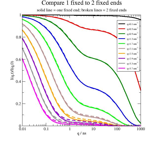
Now we compare one and two open ends. The differences are marginally and only significant at larger Q for long times as the plateau is different. The changes will be difficult to discriminate in real measurements.

import jscatter as js
import numpy as np
t = js.loglist(0.01, 1000, 50)
q=np.r_[0.1:4:0.4]
l=0.38  # nm , bond length amino acids

p=js.grace(1.5,1.5)
p.xaxis(label='q / ns',scale='log')
p.yaxis(label='I(q,t)/I(q,0)')
p.title('Compare 1 fixed to 2 fixed ends')
p.subtitle('solid line = one fixed end; broken lines = 2 fixed ends')

# two fixed ends
fFR2 = js.dynamic.fixedFiniteRouse(t, q, 124, l=l, Dcm=0.004, frict=9e-14, fixedends=2)
# one fixed end
fFR1 = js.dynamic.fixedFiniteRouse(t, q, 124, l=l, Dcm=0.004, frict=9e-14, fixedends=1)

for i, z in enumerate(fFR1, 1):
    p.plot(z.X, z.Y, line=[1, 3, i], symbol=0, legend=fr'q={z.q:.1f} nm\S-1')
for i, z in enumerate(fFR2, 1):
    p.plot(z.X, z.Y, line=[3, 3, i], symbol=0, legend='')

p.legend(x=100,y=0.95,charsize=0.6)

# p.save(js.examples.imagepath+'/fixedRouse_1vs2.jpg',size=(2,2))

jscatter.dynamic.fixedFiniteZimm(t, q, NN=None, pmax=None, l=None, Dcm=None, Dcmfkt=None, tintern=0.0, mu=0.5, viscosity=1.0, ftype=None, rk=None, Temp=293, fixedends=1)[source]

Zimm dynamics of a chain with fixed ends with internal friction and hydrodynamic interactions.

Opposite to the finiteZimm() here one or both ends are fixed. This might be a chain tethered to a particle that defines the diffusion. Chains are non interacting.

Parameters:

fixedends0,1,2, default = 1

Number of fixed ends. 0 is only for comparison and corresponds to finiteZimm() .

tarray

Time in units nanoseconds.

q: float, array

Scattering vector in units nm^-1. If q is list a dataList is returned otherwise a dataArray is returned.

NNinteger

Number of chain beads.

lfloat, default 1

Bond length between beads; units nm.

pmaxinteger, list of float, default is NN

integer => maximum mode number taken into account.
list => list of amplitudes $a_p > 0$ for individual modes to allow weighing. Not given modes have weight zero.

Dcmfloat

Center of mass diffusion in nm²/ns.

Dcmfktarray 2xN, function

Function f(q) or array with [qi, f(qi)] as correction for Dcm like Diff = Dcm*f(q). e.g. for inclusion of structure factor and hydrodynamic function with f(q)=H(Q)/S(q). Missing values are interpolated.

tinternfloat>0

Additional relaxation time due to internal friction between neighboring beads in units ns.

mufloat in range [0.01,0.99]

$\nu$ describes solvent quality.

<0.5 collapsed chain

=0.5 theta solvent 0.5 (gaussian chain)

=0.6 good solvent

>0.6 swollen chain

viscosityfloat

$\eta$ in units cPoise=mPa*s e.g. water $visc(T=293 K) =1 mPas$

Tempfloat, default 273+20

Temperature in Kelvin.

ftype‘czif’, default = ‘zif’

Type of internal friction and interaction modification.

Default Zimm is used with $t_{intern}=0$

‘zif’ Internal friction between neighboring beads in chain [3]_.

$t_{zp}=t_z p^{-3\nu}+t_{intern}$

‘czif’ Bead confining harmonic potential with internal friction, only for $\nu=0.5$ [6]_ .

The beads are confined in an additional harmonic potential with $\frac{1}{2}k_c(r_n-0)^2$ leading to a more compact configuration. $rk= k_c/k$ describes the relative strength compared to the force between beads $k$.

rkNone , float

$rk= k_c/k$ describes the relative force constant for ftype ‘czif’.

Returns:

S(q,t)/S(q,0)dataArrayfor single q, dataListfor multiple q

[time; Sqt; Sqt_inf; Sqtinc; Sqtz]
time units ns
Sqt is S(q,t)/S(q,0) coherent scattering with diffusion and mode contributions
Sqt_inf is coherent scattering with ONLY diffusion (no internal modes)
Sqtinc is incoherent scattering with diffusion and mode contributions (no separate diffusion)
Sqt0 is coherent scattering with diffusion and mode contributions, but no Dcmfkt => f(q)=1
.q wavevector
.modecontribution $a_p$ of coherent modes i in sequence as in PRL 71, 4158 equ (3)
.Re is $R_e=lN^{\nu}$
.tzimm => Zimm time or rotational correlation time
.t_p characteristic times
…. use .attr for all attributes

Notes

The Zimm model describes beads connected by harmonic springs with hydrodynamic interaction (see 4.2 in [1]). We find

\[S(q,t) = \frac{1}{N} e^{-q^2D_{cm}t}\sum_{n,m}^N e^{-\frac{1}{6}q^2B(n,m,t)}\]

$B(n,m,t)$ describes the internal motions characterised by eigenmodes of the equation 4.II.6 in [1] $\frac{\zeta_p}{\zeta} k \frac{\partial^2 \Phi_{pn}}{\partial^2 n}=-k_p\Phi_{pn}$ where $\Phi_{pn}$ describes the delocalisation of bead n in mode p.

The boundary conditions select the eigenmodes from the general form $\Phi_{pn} = A sin(kn) + Bcos(kn)$

Two free ends $\partial\Phi_{pn}/\partial n=0 \text{ for n=0 and n=N}$ select A=0 and k=pπ/N (equ. 4.II.7+9 in [1]):

\[B(n,m,t)=|n-m|^{2\nu}l^2 + \sum_{p=1}^{N-1} A_p cos(\pi pn/N)cos(\pi pm/N) (1-e^{-t/t_{zp}})\]
One fixed and one free end $\partial\Phi_{pn}/\partial n=0 \text{ at n=0 and } \Phi_{pn}=0$ at N select B=0 and k=(p-1/2)π/N (see [2]):

\[B(n,m,t)=|n-m|^{2\nu}l^2 + \sum_{p=1-1/2}^{N-1-1/2} A_p sin(\pi pn/N) sin(\pi pm/N) (1-e^{-t/t_{zp}})\]
Two fixed ends $\Phi_{pn}=0$ at n=0 and n=N select B=0 and k=pπ/N:

\[B(n,m,t)=|n-m|^{2\nu}l^2 + \sum_{p=1}^{N-1} A_p sin(\pi pn/N)sin(\pi pm/N) (1-e^{-t/t_{zp}})\]

For fixed ends the center of mass diffusion Dcm is that of the object where the chain is fixed. The chain dimension is defined by $R_e=lN^{\nu}$.

Unfortunately there are some papers that give wrong equations for fixed end Zimm or Rouse dynamics. The correct equations above can be retrieved from [1] appendix 4.II as solution of the differential equation 4.II.6 above which describes standing waves in a string or in a open tube. The classical Zimm/Rouse describe two open ends.

For detailed description of parameters see finiteZimm().

References

[1] (1,2,3,4)

The Theory of Polymer dynamics Doi, M., & Edwards, S. F. (1988). Clarendon Press.

[2]

Normal Modes of Stretched Polymer Chains Y. Marciano and F. Brochard-Wyart Macromolecules 1995, 28, 985-990 https://doi.org/10.1021/ma00108a028

Examples

Let us assume we have a core shell micelle of diblock copolymers with a hydrophobic part that assemble in the core and the hydrophilic part extended into the solvent. The core is solvent matched and invisible. For low aggregation number the hydrophobic tails extending into the solvent dont interact and the motions are that of a Zimm chain with one fixed end. The center of mass diffusion is that of the micelle and much slower than $D_{Zimm}$ but could be determined by DLS dilution series or PFG-NMR. (See e.g. Mark et al. https://doi.org/10.1103/PhysRevLett.119.047801 for silica nanoparticles with grafted chains)

For comparison we think of a triblock with hydrophobic ends that will make a loop that both ends are fixed (but not at the same position). The hydrophilic is of same size. We neglect any influence of the core onto the chain configuration.

We allow a Dcm ≈50 times slower than DZimm of the hydrophilic tail.

We observe two relaxations, a faster of the internal dynamics and a slower because of diffusion.

First compare one fixed end (full lines) with the free Zimm (broken lines). For long times the diffusion gets equal visible at low q for long times.

Obviously the amplitude of mode relaxations is much stronger than for open ends due to the different eigenmodes.

import jscatter as js
import numpy as np
t = js.loglist(0.1, 1000, 40)
q=np.r_[0.1:2:0.25]
l=0.38  # nm , bond length amino acids

p=js.grace(1.5,1.5)
p.xaxis(label='q / ns',scale='log')
p.yaxis(label='I(q,t)/I(q,0)')
p.title('Compare 1 fixed to free ends')
p.subtitle('solid line = one fixed end; broken lines = open ends')

# free ends just for comapring
fFZ0 = js.dynamic.fixedFiniteZimm(t, q, 124, 40, l=l, mu=0.5, Dcm=0.004,fixedends=0)
# one fixed end
fFZ1 = js.dynamic.fixedFiniteZimm(t, q, 124, 40, l=l, mu=0.5, Dcm=0.004,fixedends=1)

for i, z in enumerate(fFZ1, 1):
    p.plot(z.X, z.Y, line=[1, 3, i], symbol=0, legend=fr'q={z.q:.1f} nm\S-1')
for i, z in enumerate(fFZ0, 1):
    p.plot(z.X, z.Y, line=[3, 3, i], symbol=0, legend='')

p.legend(x=0.2,y=0.4,charsize=0.6)

# p.save(js.examples.imagepath+'/fixedZimm_vs_freeZimm.jpg',size=(1.,1.))

Now we compare one and two open ends. The differences are marginally and will be difficult to discriminate in real measurements.

import jscatter as js
import numpy as np
t = js.loglist(0.1, 1000, 40)
q=np.r_[0.1:2:0.25]
l=0.38  # nm , bond length amino acids

p=js.grace(1.5,1.5)
p.xaxis(label='q / ns',scale='log')
p.yaxis(label='I(q,t)/I(q,0)')
p.title('Compare 1 fixed to 2 fixed ends')
p.subtitle('solid line = one fixed end; broken lines = 2 fixed ends')

# two fixed ends
fFZ2 = js.dynamic.fixedFiniteZimm(t, q, 124, 40, l=l, mu=0.5, Dcm=0.004, fixedends=2)
# one fixed end
fFZ1 = js.dynamic.fixedFiniteZimm(t, q, 124, 40, l=l, mu=0.5, Dcm=0.004, fixedends=1)

for i, z in enumerate(fFZ1, 1):
    p.plot(z.X, z.Y, line=[1, 3, i], symbol=0, legend=fr'q={z.q:.1f} nm\S-1')
for i, z in enumerate(fFZ2, 1):
    p.plot(z.X, z.Y, line=[3, 3, i], symbol=0, legend='')

p.legend(x=0.2,y=0.4,charsize=0.6)

# p.save(js.examples.imagepath+'/fixedZimm_1vs2_fixed.jpg',size=(1,1))

jscatter.dynamic.fixedWindowScanArrhenius(Q, Temp, w, u2, A1, B1, Ea_1, tau0_1, tau_res, bgr=0, A2=0, B2=0, Ea_2=None, tau0_2=None, A3=0, B3=0, Ea_3=None, tau0_3=None)[source]

Intensities of fixed window scans assuming Arrhenius behavior of up to 3 processes for elastic and inelastic FWS. Shortcut fWSA

In case of thermally activated hindered motions the characteristic time $\tau$ of a process is represented by an Arrhenius ansatz $\tau = \tau_{\infty}e^{E_a / RT}$ [1].

If the elastic FWS has contribution of the inelastic FWS it needs to be included in the bgr.

Parameters:

Temparray, float

Temperature in Kelvin.

Qarray, float

Scattering vector in units 1/nm.

wfloat

Offset frequency $\omega_{off}$ in units 1/ns. Offset energy $\Delta E[\mu eV] /\hbar= \omega_{off}$ with js.dynamic.hbar .

u2array len(Q), float

Means square displacements for the Debye-Waller factor in 1/Q**2 units.

float : assumes u2*Temp => <u2> with given value as scaling with temperature.
dataAray : temperature dependence with Temp as X and u2 as Y . Values u2(Temp) will be linear interpolated from dataArray.

B1,B2,B3float

Intensity of the j-th process $B_j$ related to the number of atoms contributing to it.

A1,A2,A3float

EISF, elastic fraction of the j-th dynamic process contributing to elastic FWS. (1-Aj) is the inelastic part.

Ea_1,Ea_2,Ea_3float

Activation energy $E_{aj}$ of the j-th dynamic process in units meV.

tau0_1,tau0_2,tau0_3float

The high-temperature relaxation time limit of the j-th dynamic process $τ_{0j}(Q)$ in 1/ns.

tau_resfloat

1/HWHM of instrumental resolution in ns. Can be extracted from a resolution measurement at least approximately by getHWHM() or by a Lorentz fit to the resolution.

bgrarray len(Q)

For w=0 the elastic background, but for w>0 the background contribution from the wings of the resolution function.

Returns:

: dataArray: columnname ‘Temp;IFWS;IFWS1;IFWS2;IFWS3;DWF;u2’

Notes

We use here up to n=3 processes similar to [3] equ 2 + 3. If only a single measurement (one $w_{off}$) is fitted some parameters have to be fixed (Bj=1):

elastic FWS $w_{off}=0$:

\[I_{e}(Q,T) = DWF(Q) \big[ bgr_{e} + \sum_j^n B_j(Q) \Bigl\{ A_{0j}(Q) + \frac{2}{\pi} (1-A_{0j}(Q)) arctan(\frac{\tau_j(Q)}{\tau_{res}}) \Bigr\} \big]\]

inelastic FWS $w_{off}\neq 0$:

\[I_{i}(Q,T) = DWF(Q) \big[ bgr_{i} + \sum_j^n B_j(Q) \frac{1}{\pi}(1-A_{0j}(Q)) \frac{\tau_j(Q)}{1+\omega_{off}^2\tau_j^2(Q)} \big]\]

with $A_{0j}(Q)$ being the EISF of the j-th dynamic process, $\tau_{res}$ is the instrumental resolution and the Debye-Waller factor $DWF(Q)=exp(-Q^2 \langle u^2 \rangle /3)$.

\[\tau_j(Q) = \tau_{0j}(Q)exp(\frac{E_{aj}}{k_BT})\]

is the relaxation time of the j-th dynamic process. $\tau(Q)$ is related to the HWHM Γ of a Lorentzian function commonly employed to model QENS broadening $\Gamma(Q)=1/\tau(Q)$.

From [3]: The equations above rely on the assumption that the described dynamic processes follow the Arrhenius law, which is not always the case. They also assume independent motion, which otherwise would require a convolution of two processes if they influence one another. The resolution is accounted for only in terms of its width, and in the case of the IFWS can still contribute to the background and influence the scaling parameter B in eq 3 (->inelastic FWS). Therefore, initial information can be obtained from the FWS only, yet these assumptions need to be taken into account.

Connection to full inelastic scans :

For each process j the full inelastic measurement can be expressed as

\[S_j(Q,\omega) = A_{0j}(Q)\delta(Q) + (1-A_{0j}(Q)L(Q,\omega))\]

with the Lorentzian

\[L_j(Q,\omega) = \frac{1}{\pi} \frac{\tau_j(Q)}{1+\omega^2\tau^2_j(Q)}\]

The intensity with the relative contributions $B_j(Q)$ of the processes is :

\[I(Q,\omega) = [DWF(Q)\sum_j B_j(Q) S_j(Q,\omega)] \otimes R(Q,\omega)\]

where the elastic contribution is summed $A_{0}(Q)\delta(Q) = \sum_j A_{0j}(Q)\delta(Q)$ (see threeLorentz_w()). The resolution function is $R(Q, \omega)$.

References

[1]

An investigation of micro-brownian motions in polydimethylsiloxane by complementary incoherent-neutron-scattering and nuclear-magnetic-resonance experiments below room temperature. Grapengeter, H. H., Alefeld, B. & Kosfeld, R. Colloid & Polymer Science 265, (1987). https://dx.doi.org/10.1007/BF01412711

[2]

New Possibilities with Inelastic Fixed Window Scans and Linear Motor Doppler Drives on High Resolution Neutron Backscattering Spectrometers. Frick, B.; Combet, J.; Van Eijck, L. Nuclear Instruments and Methods in Physics Research Section A: Accelerators, Spectrometers, Detectors and Associated Equipment 2012, 669, 7–13. https://doi.org/10.1016/J.NIMA.2011.11.090.

[3] (1,2,3)

Quasi-Elastic Neutron Scattering of Citrate-Capped Iron Oxide Nanoparticles: Distinguishing between Ligand, Water, and Magnetic Dynamics. Plekhanov, M. S.; Thomä, S. L. J.; Magerl, A.; Appel, M.; Zobel, M.

Phys. Chem. C 2024, 128 (28), 11661–11671. https://doi.org/10.1021/acs.jpcc.4c00479.

Examples

Example data showing 2 processes.

First only one woff then both together

We allow here 2 activation energies Ea_1 dependent of woff because of e.g. temperature up and down scans resulting in different average temperatures. Parameters A1 and A2 are the same for same Q while Bi are independent for all measurements. Other parameters are for all the same.

If you know the Q dependence of Ai and Bi of a process these can be included by encapsulating this model into a small wrapper function.

Important is that the woff, tau_res are stored in the data. If separate Q values are stored in different files with Q in filename just read all and recover the Q from filename like woff.

The model can be fitted together with full scans like was done in [3] (example will follow later).

import jscatter as js
import numpy as np
fixedWindowScan = js.dynamic.fixedWindowScanArrhenius

# data with woff =0 and 3 meV; Q is found in data
fws = js.dL(js.examples.datapath +'/FWSsun_?microeV.dat.gz')
for data in fws:
   # add woff from name in µeV convert to 1/ns
   data.woff = round(float(data.name.split('_')[1].split('mic')[0])/ js.dynamic.hbar,3)
   # tau_res from resolution of instrument, could be Q dependent
   data.tau_res = 1.66  # resolution width in ns
   data.I0 = data.Y[:5].mean()  # start value for B

# only elastic contribution with two process and independent I0
fws0 = fws.filter(woff=0)

fws0.makeErrPlot(yscale='log',residuals='relative')
# resonable limits
fws0.setlimit(u2=[0,1,0,2],bgr=[0],I0=[0,10])
fws0.setlimit(A1=[0,1], B1=[0,10],Ea_1=[50,500],tau0_1=[0,0.01])
fws0.setlimit(A2=[0,1], B2=[0,10],Ea_2=[0,50],tau0_2=[0,0.02])
fws0.setlimit(A3=[0,1], B3=[0,10],Ea_3=[50,500],tau0_3=[0,0.02])

# create reasonable starting values, use tolist to get list
I0 = fws0.I0.array
I0[I0<1] *=50
fws0.fit(model=fixedWindowScan,
            freepar={'bgr':[0.004],'u2':0.0002,
                     'A1':[.15,'Q'], 'B1':I0.tolist(), 'Ea_1':270, 'tau0_1':2e-5,
                     'A2':[0.05,'Q'], 'B2':[0.03], 'Ea_2':30, 'tau0_2':1e-2,
                     },
            fixpar={'A3':.05, 'B3':0, 'Ea_3':200, 'tau0_3':0.00001},
            mapNames={'Temp':'X','w':'woff'},workers=0)  # ,method='Nelder-Mead')

# EFWS + IFWS fit together with two process and independent I0
fws.makeErrPlot(yscale='log',residuals='relative')
# resonable limits
fws.setlimit(u2=[0,1,0,2],bgr=[0],I0=[0,10])
fws.setlimit(A1=[0,1], B1=[0,10],Ea_1=[50,500],tau0_1=[0,0.01])
fws.setlimit(A2=[0,1], B2=[0,10],Ea_2=[0,50],tau0_2=[0,0.02])
fws.setlimit(A3=[0,1], B3=[0,10],Ea_3=[50,500],tau0_3=[0,0.02])

# create reasonable starting values, use tolist to get list
I0 = fws.I0.array
I0[I0<1] *=50
fws.fit(model=fixedWindowScan,
            freepar={'bgr':[0.004,0.001,'woff'],'u2':0.0002, #'I0':fws.I0,
                     'A1':[.15,'Q'], 'B1':I0.tolist(), 'Ea_1':[270,210,'woff'], 'tau0_1':2e-5,
                     'A2':[0.05,'Q'], 'B2':[0.03], 'Ea_2':30, 'tau0_2':1e-2,
                     },
            fixpar={'A3':.05, 'B3':0, 'Ea_3':200, 'tau0_3':0.00001},
            mapNames={'Temp':'X','w':'woff'},workers=0)  # ,method='Nelder-Mead')

fws.errplot.legend(x=5,y=3,charsize=0.5)
# fws.savelastErrPlot(js.examples.imagepath+'/fixedWindoScanfit.jpg', size=(2,1),dpi=600)

jscatter.dynamic.frequency2timeFF(data, resolution_t=None, dt=None, tfactor=1, Qname='Q')[source]

Fourier transform from frequency domain (experiment) to time domain for inelastic neutron scattering.

Based/inspired of unift from Reiner Zorn (now the core FT is f95 and uses openMP). Designed for Fourier transform (FT) of inelastic neutron scattering data into the time domain. It is designed to use data from backscattering- as well as time-of-flight spectrometers.

Shortcut f2tFF calls this function. Data need to be in constant Q fashion.

Parameters:

datadataArrays, dataList

$I(t,f)$ from measurement in frequency domain in units of 1/ns. Data need to be in constant Q fashion, NOT constant angle and we assume positive .X values as gain side of the spectrum. Use convert_e2w() to convert to 1/ns.

resolution_tdataArray

FT of resolution measurements with X in units ns. If given dt and tfactor are ignored. This is used to get same timescale as FT of resolution.

dtfloat, default =None

Times step for the result in units ns.

Default $dt =\pi/max(|f_i|) = h/(2 E_{max})$ .

tfactorfloat, default = 1

Factor to increase $t_{max}$ by factor.

We use $t_{max} = 1/FWHM=1/2HWHM$ of the resolution. HWHM is determined in shiftAndBinning() for resolution. Without resolution we use $t_{max} = 1 ns$ .

e.g. 1 ns for SPHERES@MLZ with $t_{max}\Delta\hbar\omega\approx 0.7 \mu eV$

Qnamestring, default ‘Q’

Attribute name of the wavevector to find correct wavevector.

Returns:

I(q,t)dataArray or dataList

5 columns with ‘times; abs(Iqt) ; error Iqt; real Iqt ;imag Iqt’
columnname = ‘t;Iqt;eIqt;Iqtreal;Iqtimag’
t = [0:tmax:dt]
attributes of data

Notes

Fourier transform (FT) of inelastic neutron scattering data into the time domain as

\[I(Q,t) = \int_{-\infty}^{\infty} S(Q, \omega) e^{-i\omega t} d\omega\]

It is designed to use data from backscattering- as well as time-of-flight spectrometers.

In comparison to a equidistant discrete FT, e.g. by fast FT algorithms, it offers certain advantages ($E=\hbar \omega$):

A non-equidistant energy transfer E scale is allowed.
The calculation is based on representing FT by a trapezoidal-rule-like integral to avoid effects from the choice of the E grid.
Deconvolution in time-domain is done by calculating (in principle)

\[I(Q,t) = { I_{\rm exp} (Q,t) \over R(Q,t) }\]

where $I_{\rm exp} (Q,t)$ is the FT of the sample spectrum and $R(Q,t)$ that of the resolution spectrum.
The time step of the resulting data set is chosen from the available E range in order to avoid background influence (for $t\ne0$) and minimise cut-off effects (‘wiggles’).
Errors of I(Q,t) are calculated (by naive error propagation).

Actually we calculate $| I(Q,t) |$ which, if calculated with the detailed balance factor, should be equal to $I(Q,t)$. Nevertheless, the use of the absolute value offers one additional advantage:

An arbitrary shift of the sample spectrum with respect to the resolution is implicitly cancelled.

The only case in which the use of the real part could be more appropriate is if a linearly sloped background is present. In this case $real( I(Q,t))$ is free from an influence because of symmetry.

Data need be prepared before FT:

Q average, selection using mergeAttribut() to average Q values to enhance statistics.
The E range can be restricted/binned to avoid bad data close to the instrument limit using prune().
The detailed balance factor appropriate for the measuring temperature can be applied to obtain a ‘classical-approximation’ $I(Q,t)$ (see convert_e2w()).
Convert to 1/ns.
The energy loss (of the neutron, E<0) side can be reconstructed by mirroring from the E>0 side (‘mirroring’ see mirror_w()).
The peak should be shifted to zero and one may apply binnig in time shiftAndBinning().
E scale can be inverted by data.X = - data.X for each dataArray.

Examples

We use the .inx format in the example. Ask the instrument responsible for the actual meaning of values in the format and to get constant Q instead of constant angle data.

Here for SPHERES@MLZ energy is in units µeV.

The sample was a protein (alcohol dehydrogenase) in D2O buffer (see http://dx.doi.org/10.1063/1.4928512]). At these larger Q we see the combined effect of translational+rotational diffusion including slow domain motions on several 10 ns timescale. Additional there is faster dynamics of protons that needs a more complex model including TOF data. Also the signal is weak for 50mg/ml concentration.

Elastic scattering from empty can and D2O background need to be subtracted correctly. Here we do just a simplified evaluation subtracting the D2O meausrement as example.

import jscatter as js
import numpy as np

def readinx(filename,block, l2p):
    # reusable function for inx reading
    # neutron scatterers use strange data formats like .inx dependent on local contact
    # the blocks start with  number of channels. Spaces (' 562 ') are important to find the starting line.
    # this might dependent on instrument
    data = js.dL(filename,
                 block=block,                    # this finds the starting of the blocks of all angles or Q
                 usecols=[1,2,3],                # ignore the numbering at each line
                 lines2parameter=l2p)  # catch the parameters at beginning
    for da in data:
        da.channels = da.line_1[0]
        da.Q = da.line_3[0]                       # in 1/A
        da.incident_energy = da.line_3[1]         # in meV
        da.temperature = da.line_3[3]             # in K if given
    return data

# read data
vana = readinx(js.examples.datapath +'/Vana.inx.gz',block=' 562 ',l2p=[-1,-2,-3,-4])
adh = readinx(js.examples.datapath +'/ADH.inx.gz',block=' 563 ',l2p=[-1,-2,-3,-4,-5])
d2o = readinx(js.examples.datapath +'/D2O.inx.gz',block=' 562 ',l2p=[-1,-2,-3,-4])
trans = 0.95  # just a guess
for a,d in zip(adh,d2o):
   # subtract D2O measurement ( should be more complicated with transmission and also empty cell.....)
   a.eY = ((a.eY/a.Y)**2 + (d.eY/d.Y)**2)**0.5
   a.Y = a.Y - d.Y * trans
   a.eY = a.eY *a.Y

# convert to 1/ns, we can select parts of the data
vanaf = js.dynamic.convert_e2w(vana[1:-2],T=293,unit='μeV')
adhf = js.dynamic.convert_e2w(adh[1:-2],293,unit='μeV')

# shift peaks to center 0 determined from vanadium, HWHM is determined for resolution
vanaf = js.dynamic.shiftAndBinning(vanaf)
# use resolution w0 for shifting
adhf = js.dynamic.shiftAndBinning(adhf,w0=vanaf)

# FT to timedomain of resolution
vanat = js.dynamic.frequency2timeFF(data=vanaf, tfactor=1)
# FT of data, Q is used to find correct resolution
adht = js.dynamic.frequency2timeFF(data=adhf,resolution_t=vanat)

p= js.grace(2,1)
p.multi(1,3)
p[0].title('resolution')
p[0].plot(vanat,le='$Q \cE\C\S-1')
p[0].yaxis(label='I(Q,t)',scale='norm')
p[0].xaxis(label='t / ns',min=0,max=2)
p[0].legend(x=1.2,y=350)

p[1].title('protein')
p[1].subtitle(r'different t\smax\N reflext resolution HWHM')
p[2].title('diffusion coefficient')
for c,sam in enumerate(adht,1):
   # Q*Q*t shows if we see diffusion
   sam.setlimit(D=[0],beta=[0,1])
   sam.fit(js.dynamic.simpleDiffusion,{'beta':0.9,'D':1},{},{'t':'X','q':'Q'},xslice=slice(1,None))
   p[1].plot(sam.X,sam.Y,sy=[1,0.4,c])
   p[1].plot(sam.lastfit.X,sam.lastfit.Y,sy=0,li=[1,1,c])

p[1].xaxis(label=r't / ns',min=0,max=1.5)
p[1].yaxis(scale='log',min=0.01,max=1)
p[2].plot(adht.Q,adht.D,adht.D_err)
p[2].xaxis(label=r'Q / nm\S-1',min=0,max=2)
p[2].yaxis(label=[r'D / \cE\C\S2\N/ns',1,'opposite'],min=0,max=5)
# p.save(js.examples.imagepath+'/frequency2timeFF.jpg', size=(2,1),dpi=600)

jscatter.dynamic.getHWHM(data, center=0, gap=0)[source]

Find half width at half maximum (left/right) of a distribution around center.

The hwhm is determined from linear spline between Y values to find (Y.max-Y.min)/2 left and right of the max value. Requirement increasing X values and a flat background. If nothing is found an empty list is returned.

For sparse data a fit with a peak function like a Gaussian/Lorentzian is preferred.

Parameters:

datadataArray: Distribution
center: float, default=0: Center (symmetry point) of data. If None the position of the maximum is used.
gapfloat, default 0: Exclude values around center as it may contain a singularity. Excludes values within X<= abs(center-gap). The gap should be large enough to reach the baseline on left/right peak side.

Returns:

list of float with hwhm X>0 , X<0 if existing

Examples

import jscatter as js
import numpy as np

x = np.r_[0:10:200j]
data = js.formel.gauss(x,3,0.3)
data.Y += 2
HWHM = js.dynamic.getHWHM(data,3,0.1)
# => (2*np.log(2))**0.5*0.3 = 1.177 * sigma = 0.353

jscatter.dynamic.integralZimm(t, q, Temp=293, viscosity=0.001, amp=1, rtol=0.02, tol=0.02, limit=50)[source]

Conformational dynamics of an ideal chain with hydrodynamic interaction, coherent scattering.

Integral version Zimm dynamics.

Parameters:

tarray: Time points in ns
qfloat: Wavevector in 1/nm
Tempfloat: Temperature in K
viscosityfloat: Viscosity in cP=mPa*s
ampfloat: Amplitude
rtol,tolfloat: Relative and absolute tolerance in scipy.integrate.quad
limitint: Limit in scipy.integrate.quad.

Returns:

dataArray

Notes

The Zimm model describes the conformational dynamics of an ideal chain with hydrodynamic interaction between beads. We use equ 85 and 86 from [1] as

\[S(Q,t) = \frac{12}{Q^2l^2} \int_0^{\infty} e^{-u-(\Omega_Z t)^{2/3} g(u(\Omega_Z t)^{2/3})} du\]

with

\[g(y) = \frac{2}{\pi} \int_0^{\infty} x^{-2}cos(xy)(1-e^{-2^{-0.5}x^{2/3}}) dx\]

\[\Omega_z = \frac{kTQ^3}{6\pi\eta_s}\]

See [1] for details.

References

[1] (1,2)

Neutron Spin Echo Investigations on the Segmental Dynamics of Polymers in Melts, Networks and Solutions in Neutron Spin Echo Spectroscopy Viscoelasticity Rheology Volume 134 of the series Advances in Polymer Science pp 1-129 DOI 10.1007/3-540-68449-2_1

Examples

import jscatter as js
import numpy as np
t=np.r_[0:10:0.2]
p=js.grace()
for q in np.r_[0.26,0.40,0.53,0.79,1.06]:
   iqt=js.dynamic.integralZimm(t=t,q=q,viscosity=0.2e-3)
   p.plot((iqt.X*iqt.q**3)**(2/3.),iqt.Y)
p.xaxis(label=r'(Q\S3\Nt)\S2/3')
p.yaxis(label=r'I(Q,t)/I(Q,0)')
p.title('integral Zimm rescaled by characteristic time')
# p.save(js.examples.imagepath+'/integralZimm.jpg')

jscatter.dynamic.jumpDiff_w(w, q, t0, r0)[source]

Jump diffusion; dynamic structure factor in w domain.

Jump diffusion as a Markovian random walk. Jump length distribution is a Gaussian with width r0 and jump rate distribution with width G (Poisson). Diffusion coefficient D=r0**2/2t0.

Parameters:

warray: Frequencies in 1/ns
qfloat: Wavevector in nm**-1
t0float: Mean residence time in a Poisson distribution of jump times. In units ns. G = 1/tg = Mean jump rate
r0float: Root mean square jump length in 3 dimensions <r**2> = 3*r_0**2

Returns:

dataArray

Notes

Equ 6 + 8 in [1] :

\[ \begin{align}\begin{aligned}S_{inc}(q,\omega) = \frac{1}{\pi} \frac{\Delta\omega}{\Delta\omega^2 + \omega^2}\\with \; \Delta\omega = \frac{1-e^{-q^2 r_0^2/2}}{t_0}\end{aligned}\end{align} \]

References

[1]

Incoherent neutron scattering functions for random jump diffusion in bounded and infinite media. Hall, P. L. & Ross, D. K. Mol. Phys. 42, 637–682 (1981).

jscatter.dynamic.jumpDiffusion(t, Q, t0, l0)[source]

Incoherent intermediate scattering function of translational jump diffusion in the time domain.

Parameters:

tarray: Times, units ns
Qfloat: Wavevector, units nm
t0float: Residence time, units ns
l0float: Mean square jump length, units nm

Returns:

dataArray

Notes

We use equ. 3-5 from [1] for random jump diffusion as

\[T(Q,t) = exp(-\Gamma(Q)t)\]

with residence time $\tau_0$ and mean jump length $<l^2>^{1/2}_{av}$ and diffusion constant $D$ in

\[\Gamma(Q) = \frac{DQ^2}{1+DQ^2\tau_0}\]

\[D=\frac{ <l^2>_{av}}{6\tau_0}\]

References

[1]

Experimental determination of the nature of diffusive motions of water molecules at low temperatures J. Teixeira, M.-C. Bellissent-Funel, S. H. Chen, and A. J. Dianoux Phys. Rev. A 31, 1913 – Published 1 March 1985

jscatter.dynamic.linearChainORZ(t, q, N=100, l=1, fa=None, Dcm=None, Dcmfkt=None, viscosity=1, costheta=0.0, T=293, reducedfriction=0.25, tintern=0)[source]

Dynamics of a linear polymer chain using optimized Rouse-Zimm approximation (ORZ).

The linear dynamic structure factor is calculated in analogy to the star described by Guenza [1].

The linear chain dynamics is decribed within the more general optimized Rouse-Zimm (ORZ) approximation introduced by Bixon and Zwanzig [3] [4] . See solveOptimizedRouseZimm().

We extend this here using bead scattering lengths for partial matching and allow individual bond correlations.

To speedup fitting use the memoize function as described in memoize().

Parameters:

tarray

timepoints in units ns.

qarray

Scattering vectors in units 1/nm.

Nint

Number of beads .

lfloat, default = 0.38 nm (amino acid)

Bond length or Kuhn length in units nm.

faNone, list of float

Scattering length of bead/monomer $fa_i$. Can be used to match parts of the star to the solvent.

None : Equal 1 for all beads.
list: length N as scattering length of beads in sequence

Dcmfloat

Center of mass diffusion in units nm**2/ns. If None the calculated value D_ORZ is used.

Dcmfktarray 2xN, function

Function f(q) or array with [qi, f(qi) ] as correction for Dcm like Diff = Dcm*f(q). e.g. for inclusion of structure factor or hydrodynamic function with f(q)=H(Q)/S(q). Missing values are interpolated.

costhetafloat, list of float, 0 <= costheta < 1

Cos of bond correlation angle $\langle \vec{l_i} \cdot \vec{l_j} \rangle /l^2 = cos(theta)$ between normalized bonds $l_i$ with $0 \le cos(\theta) \le 1$.

costheta = 0 : FJC (freely jointed chain) model, no bond correlation, Rouse dynamics, No HI .
float $0 < cos(\theta) \le 1$ : FRC (free rotating chain). With $R_{ee} = Nl^2C_{\infty}=Nl^2 \frac{1+cos(\theta)}{1-cos(\theta)}$ .
list of float length N-2 : FRC with individual $cos(\theta_i)$ for each pair of N-2 bonds.
- costheta=([0.1]*24+[0.7]*24) for stretched beginning and flexible end of 50 beads.
- costheta=0.8 * np.cos(np.pi*np.r_[:1:(N-2)*1j])**2 + 0.1 for flexible center and stretched ends.
For fitting encapsulate the model in a function where you parametrize your model for costheta .
During fits use limits(costheta=[None,None,0.001,0.999]) to avoid singular matrices.

e.g. (from [5] p. 53) $C_{\infty} | Kuhn length [A] | cos(theta)$

polyisoprene 4.6 | 8.2 | 0.783

polyethylene oxide 6.7 | 11 | 0.85

polyethylene 7.4 | 14 | 0.865

atactic polystyrene 9.5 | 18 | 0.895

viscosityfloat, default=1 (H2O@20C )

$\eta$ in units cPoise=mPa*s e.g. water $visc(T=293 K) =1 mPas$

Tfloat, default 273+20

Temperature in Kelvin.

reducedfrictionfloat, default 0.25

Reduced friction $\zeta_r = \zeta/6\pi\eta_sl$ in hydrodynamic tensor H.

=0 : free draining limit, no HI, Rouse dynamics.
>0 : with HI typically <0.5. For h>0.5 we get negative eigenvalues.

See solveOptimizedRouseZimm().

During fits use limits(reducedfriction=[0,0.43,0.,0.5]) to avoid singular matrices.

tinternfloat>0, default 0

Relaxation time due to internal friction between neighboring beads in ns.

Returns:

sqtdataList

Intermediate scattering function of a star for given q.

[times; Sqt; Sqt only diffusion; Sqt cumulant]
columnname = ‘t;Sqt;Sqt_inf;Sqt_cum’
.q : scattering vector
.D_ORZcum : diffusion coefficinet in initial slope (cumulant)
.D_ORZ : translational diffusion ORZ model
.Dcm : used center of friction/mass diffusion
.Fq : form factor
.Fq_inf : form factor t=inf
.beadfriction : bead friction
.bondrateconstant : bondrateconstant in 1/ns
.moderelaxationtimes : used moderelaxationtimes in ns [4] equ 2.17
.mode_rmsd : used mode rmsd as math:`l/mu^{0.5} # [4] equ 2.19
.reducedfriction : reducedfriction
.costheta : costheta
.eigenvalues : all evals
.mu : all mu
.l : bondlength l
.N : Number of beads
.Rg : radius of gyration in nm
.Rg_red : reduced radius of gyration

Notes

See solveOptimizedRouseZimm() for a description of the ORZ model with respective parameters and the dynamic structure factor $S(q,t)/S(q,0)$ .

Here we use a linear chain with N beads and set elements $U^{-1}_{ij} <0.001 \rightarrow 0$.

The inverse of the static bond correlation matrix $U_{ij}^{-1} = \langle l_i\cdot l_j\rangle /l^2$ in dimesionless form is

\[\begin{split}U_{ij}^{-1} &= \delta_{i,j} &\text{ for uncorrelated bonds } \\ &= \prod_{n=i}^{j} g_n \; &\text{ for individual } g_i \text{ including constant g}\end{split}\]

The transfer matrix M is

\[M = \delta_{i,j} - \delta_{i+1,j}\]

References

[1]

Static and Dynamic Structure Factors for Star Polymers in θ Conditions. Guenza, M. & Perico, A. Macromolecules 26, 4196–4202 (1993). https://doi.org/10.1021/ma00068a020

[2]

A Local Approach to the Dynamics of Star Polymers. Guenza, M., Mormino, M. & Perico, A. Macromolecules 24, 6168–6174 (1991). https://doi.org/10.1021/ma00023a018

[3]

Theoretical basis for the Rouse‐Zimm model in polymer solution dynamics. Zwanzig, R. The Journal of Chemical Physics 60, 2717–2720 (1974) https://doi.org/10.1063/1.1681433

[4]

A hierarchy of models for the dynamics of polymer chains in dilute solution. Perico, A., Ganazzoli, F. & Allegra, G. The Journal of Chemical Physics 87, 3677–3686 (1987). https://doi.org/10.1063/1.452966

[5]

Rubinstein, M. & Colby, R. H. Polymer Physics. (OUP Oxford, 2003).

[6]

Intramolecular relaxation dynamics in semiflexible dendrimers. Kumar, A. & Biswas, P. Journal of Chemical Physics 134, (2011). https://doi.org/10.1063/1.3598336

Examples

Here we examine how changig stiffness influences dynamics.

import jscatter as js
import numpy as np

q= np.r_[0.01,0.1:2:0.2]
t = np.r_[0:1:0.02,1:20:1,20:100:5]

def stiffendschain(t, q, N, l=0.5, cosmin =0.05,cosmax=0.8,rf=0.25):
   costheta = (cosmax-cosmin) * np.cos(np.pi*np.r_[:1:(N-2)*1j])**2 + cosmin
   sqt = js.dynamic.linearChainORZ(t, q, N, l=0.5, costheta = costheta , reducedfriction=rf)
   return sqt

p = js.grace()
p.xaxis(label='t / ns')

sqt = stiffendschain(t, q, 100, l=1, cosmin =0.1,cosmax=0.5)
for c,sq in enumerate(sqt,1):
    p.plot(sq.X,sq._Sqt,li=[1,1,c],sy=0,le=f'{sq.q:.2f} nm\\S-1')

sqt = stiffendschain(t, q, 100, l=1, cosmin =0.1,cosmax=0.1)
for c,sq in enumerate(sqt,1):
    p.plot(sq.X,sq._Sqt,li=[3,1,c],sy=0,le='')

p.yaxis(label='S(Q,t),S(Q,0)',scale='log',min=0.01,max=1)
p.legend(charsize=0.7)
p.title('chain with stiff ends ')
p.subtitle('solid: stiff ends; broken: flexible ends')

# p.save(js.examples.imagepath+'/ORZ_linearstiffends.png',size=(1.5,1.5),dpi=300)

jscatter.dynamic.lorentz_w(w, hwhm)[source]

Normalized Lorentz function.

\[Ln(w) = \frac{\gamma}{\pi(w^2+\gamma^2)}\]

Same as KWW in frequency domain as Fourier tranform of stretched exponential with beta=1.

Parameters:

warray: Frequency
hwhmfloat: Half width half maximum $\gamma$ or relaxation rate.

Returns:

dataArray

Examples

import jscatter as js
import numpy as np

w = np.r_[-100:100:0.1]
p = js.grace(2,2)
for hw in np.r_[1:32:5]:
    iw = js.dynamic.lorentz_w(w,hw)
    p.plot(iw,le=f'hw={hw}')

p.yaxis(scale='l',label=r'S(\xw\f{}) / a.u.',min=1e-5,max=1)
p.xaxis(label=r'\xw\f{} / ns\S-1',min=-100,max=100)
p.legend(x=30,y=1,charsize=0.8)
# p.save(js.examples.imagepath+'/lorentz_w.jpg', size=(2,2))

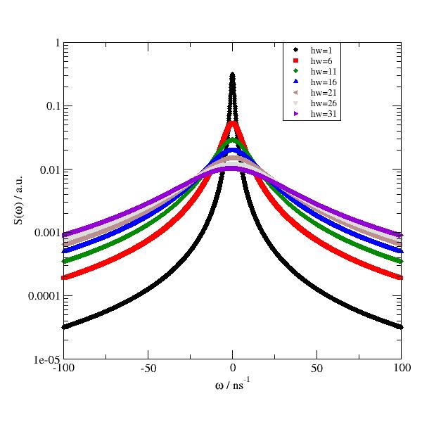
jscatter.dynamic.methylRotation(t, q, t0=0.001, fraction=1, rhh=0.12, beta=0.8)[source]

Incoherent intermediate scattering function of CH3 methyl rotation in the time domain.

Parameters:

tarray: List of times, units ns
qfloat: Wavevector, units nm
t0float, default 0.001: Residence time, units ns
fractionfloat, default 1: Fraction of protons contributing.
rhhfloat, default=0.12: Mean square jump length, units nm
betafloat, default 0.8: exponent

Returns:

dataArray

Notes

According to [1]:

\[I(q,t) = (EISF + (1-EISF) e^{-(\frac{t}{t_0})^{\beta}} )\]

\[EISF=\frac{1}{3}+\frac{2}{3}\frac{sin(qr_{HH})}{qr_{HH}}\]

with $t_0$ residence time, $r_{HH}$ proton jump distance.

References

[1]

Bée, Quasielastic Neutron Scattering (Adam Hilger, 1988).

[2]

Monkenbusch et al. J. Chem. Phys. 143, 075101 (2015)

Examples

import jscatter as js
import numpy as np
# make a plot of the spectrum
w=np.r_[-100:100]
ql=np.r_[1:15:1]
iqwCH3=js.dL([js.dynamic.time2frequencyFF(js.dynamic.methylRotation,'elastic',w=np.r_[-100:100:0.1],q=q )
                                            for q in ql])
p=js.grace()
p.plot(iqwCH3,le='CH3')
p.yaxis(min=1e-5,max=10,scale='l')

jscatter.dynamic.mirror_w(data, emin=0)[source]

Mirrors w spectra from energy gain to energy loss side. NOT in place.

Might be needed only for TOF data.

Because of the difference between energy gain and loss side first use convert_e2w() and then mirror in frequency domain.

Parameters:

datadataArray, dataList

Data to mirror.

We assume positive frequencies as gain side of the spectrum. If not use data.X = - data.X to convert.

eminfloat, default 0

Border where to mirror. We use -emin as border on loss side.

Returns:

mirrored datadataArray

Notes

As this is inspiredd from unift (Reiner Zorn) a short description from unift:

Enter a positive value $E_{min}$ to indicate that $S(Q,E)$ for $E<-E_{min}$ should be replaced by $S(Q,-E)$, i.e. ‘mirrored’ from the energy gain side. This improves the treatment of TOF data significantly because there the energy loss side is truncated more closely to the elastic line that the energy gain side. The choice of $E_{min}$ requires some inspection of the $S(Q,\omega)$ data to find a place where it can be done without introducing a discontinuity.

jscatter.dynamic.multiArmStarORZ(t, q, f_arm=4, n_arm=10, l=1, fa=None, Dcm=None, Dcmfkt=None, viscosity=1, costheta=0.0, T=293, reducedfriction=0.25, tintern=0)[source]

Dynamics of a symmetric multi arm star of polymer chains using optimized Rouse-Zimm approximation (ORZ).

The star dynamic structure factor is explicitly described by Guenza [1] and extended to partially stretched stars in [2].

The star polymer dynamics is decribed within the more general optimized Rouse-Zimm (ORZ) approximation introduced by Bixon and Zwanzig [3] [4] . See solveOptimizedRouseZimm().

We extend this here using bead scattering lengths for partial matching and allow individual bond correlations.

To speedup fitting use the memoize function as described in memoize().

Parameters:

tarray

timepoints in units ns.

qarray

Scattering vectors in units 1/nm.

f_armint

Number of arms $f_{arm}$.

n_armint

Number of beads per arm $n_{arm}$ excluding the center common for all arms.

lfloat, default = 0.38 nm (amino acid)

Bond length or Kuhn length in units nm.

faNone, list of float

Scattering length of bead/monomer $fa_i$. Can be used to match parts of the star to the solvent.

None : Equal 1 for all beads.
list: length (1 + f_arm * n_arm) as scattering length of beads in sequence [center, 1..n_arm first arm,1..n_arm second arm,….]

e.g. fa=[0] + ([0]*5+[1]*6)*4 for a 4 arm star of 11 beads per arm with the center and 5 innermost beads matched.

Dcmfloat

Center of mass diffusion in units nm**2/ns. If None the calculated value D_ORZ is used.

Dcmfktarray 2xN, function

Function f(q) or array with [qi, f(qi) ] as correction for Dcm like Diff = Dcm*f(q). e.g. for inclusion of structure factor or hydrodynamic function with f(q)=H(Q)/S(q). Missing values are interpolated.

costhetafloat, list of float, 0 <= costheta < 0.1

Cos of bond correlation angle $\langle \vec{l_i} \cdot \vec{l_j} \rangle /l^2 = cos(theta)$ between normalized bonds $l_i$ with $0 \le cos(\theta) \le 1$.

costheta = 0 : FJC (freely jointed chain) model, no bond correlation, Rouse dynamics, No HI .
float $0 < cos(\theta) \le 1$ : FRC (free rotating chain). With $R_{ee} = Nl^2C_{\infty}=Nl^2 \frac{1+cos(\theta)}{1-cos(\theta)}$ .
list of float length N-2 : FRC with individual $cos(\theta_i)$ for each pair of N-2 bonds.
- costheta=([0.1]*24+[0.7]*24) for stretched beginning and flexible end of 50 beads.
- costheta=0.8 * np.cos(np.pi*np.r_[:1:(N-2)*1j])**2 + 0.1 for flexible center and stretched ends.
For fitting encapsulate the model in a function where you parametrize your model for costheta .
During fits use limits(costheta=[None,None,0.001,0.999]) to avoid singular matrices.

e.g. (from [5] p. 53) $C_{\infty} | Kuhn length [A] | cos(theta)$

polyisoprene 4.6 | 8.2 | 0.783

polyethylene oxide 6.7 | 11 | 0.85

polyethylene 7.4 | 14 | 0.865

atactic polystyrene 9.5 | 18 | 0.895

viscosityfloat, default=1 (H2O@20C )

$\eta$ in units cPoise=mPa*s e.g. water $visc(T=293 K) =1 mPas$

Tfloat, default 273+20

Temperature in Kelvin.

reducedfrictionfloat, default 0.25

Reduced friction $\zeta_r = \zeta/6\pi\eta_sl$ in hydrodynamic tensor H.

=0 : free draining limit, no HI, Rouse dynamics.
>0 : with HI typically <0.5. For h>0.5 we get negative eigenvalues.

See solveOptimizedRouseZimm().

During fits use limits(reducedfriction=[0,0.43,0.,0.5]) to avoid singular matrices.

tinternfloat>0, default 0

Relaxation time due to internal friction between neighboring beads in ns.

Returns:

sqtdataList

Intermediate scattering function of a star for given q.

[times; Sqt; Sqt only diffusion; Sqt cumulant]
columnname = ‘t;Sqt;Sqt_inf;Sqt_cum’
.q : scattering vector
.D_ORZcum : diffusion coefficinet in initial slope (cumulant)
.D_ORZ : translational diffusion ORZ model
.Dcm : used center of friction/mass diffusion
.Fq : normalized form factor
.Fq_inf : normalized form factor t=inf
.beadfriction : bead friction
.bondrateconstant : bondrateconstant in 1/ns
.moderelaxationtimes : used moderelaxationtimes in ns [4] equ 2.17
.mode_rmsd : used mode rmsd as math:`l/mu^{0.5} # [4] equ 2.19
.reducedfriction : reducedfriction
.costheta : costheta
.eigenvalues : all evals
.mu : all mu
.l : bondlength l
.N : Number of beads
.Rg : radius of gyration in nm
.Rg_red : reduced radius of gyration

Notes

See solveOptimizedRouseZimm() for a description of the ORZ model with respective parameters and the dynamic structure factor $S(q,t)/S(q,0)$ .

Here we use a symetric star with f_arm arms of each n_arm beads and a connecting bead as described by Guenza [1] and set elements $U^{-1}_{ij} <0.001 \rightarrow 0$.

The inverse of the static bond correlation matrix $U_{ij}^{-1} = \langle l_i\cdot l_j\rangle /l^2$ in dimesionless form is

\[\begin{split}U_{ij}^{-1} &= \delta_{i,j} &\text{ for uncorrelated bonds } \\\end{split}\]

For individual $g_i$ including that g all are the same and core $g_0$ (indexing start at 1)

\[\begin{split}U_{ij}^{-1} &= \prod_{n=i}^{j} g_n &\text{ for i,j on the same arm} \\ &= g_0 \prod_{n=1}^{j} g_n \prod_{m=1}^{i} g_m &\text{ for i,j on different arms}\end{split}\]

The transfer matrix M is (ignoring the not used $M_{1i}$) accordig to [2] :

\[\begin{split}\begin{align} &M_{1,i} &= 1/N &\text{ for }i=1..n_{arm} \\ &M_{i,i} &= 1 &\text{ for }i=2..n_{arm} \\ &M_{i+1,i} &= -1 &\text{ for }i=2..n_{arm},n_{arm}+2..2n_{arm},...,(f_{arm}-1)N+2...f_{arm}n_{arm} \\ &M_{i,1} &= -1 &\text{ for }i=2, n_{arm}+2,2n_{arm}+2,...,(f_{arm}-1)N+2 \\ &M_{i,j} &= 0 &\text{ all others} \end{align}\end{split}\]

References

[1] (1,2)

Static and Dynamic Structure Factors for Star Polymers in θ Conditions. Guenza, M. & Perico, A. Macromolecules 26, 4196–4202 (1993). https://doi.org/10.1021/ma00068a020

[2] (1,2)

A Local Approach to the Dynamics of Star Polymers. Guenza, M., Mormino, M. & Perico, A. Macromolecules 24, 6168–6174 (1991). https://doi.org/10.1021/ma00023a018

[3]

Theoretical basis for the Rouse‐Zimm model in polymer solution dynamics. Zwanzig, R. The Journal of Chemical Physics 60, 2717–2720 (1974) https://doi.org/10.1063/1.1681433

[4]

A hierarchy of models for the dynamics of polymer chains in dilute solution. Perico, A., Ganazzoli, F. & Allegra, G. The Journal of Chemical Physics 87, 3677–3686 (1987). https://doi.org/10.1063/1.452966

[5]

Rubinstein, M. & Colby, R. H. Polymer Physics. (OUP Oxford, 2003).

[6]

Intramolecular relaxation dynamics in semiflexible dendrimers. Kumar, A. & Biswas, P. Journal of Chemical Physics 134, (2011). https://doi.org/10.1063/1.3598336

Examples

Here we compare the FJC with FRC (costheta=0.1) of a 5 arm star in water. We see the tranlational diffusion component at longer times (extrapolated to short times) and the faster relaxation of internal modes at short times approaching the cumulant at shortest times.

import jscatter as js
import numpy as np

q= np.r_[0.01,0.1:2:0.2]
t = np.r_[0:1:0.02,1:20:1,20:400:5]

p = js.grace()
p.xaxis(label='t / ns')

sqt = js.dynamic.multiArmStarORZ(t, q, 5, 50, l=0.5, costheta = 0, reducedfriction=0.)
tt = t<20  # for cumulant
for c,sq in enumerate(sqt,1):
    p.plot(sq.X,sq._Sqt,li=[1,1,c],sy=0,le=f'{sq.q:.2f} nm\S-1')
    p.plot(sq.X, sq._Sqt_inf, li=[2, 1, c], sy=0, )
    p.plot(sq.X[tt], sq._Sqt_cum[tt], li=[2, 1, 1], sy=0, )

# small
sqt = js.dynamic.multiArmStarORZ(t, q, 5, 50, l=0.5, costheta = 0.1, reducedfriction=0)
for c,sq in enumerate(sqt,1):
    p.plot(sq.X,sq._Sqt,li=[3,1,c],sy=0)

p.yaxis(label='S(Q,t),S(Q,0)',scale='log',min=0.01,max=1)
p.legend(charsize=0.7)
p.title('5 arm star ORZ model: no HI and costheta=0, 0.1')
p.text('trans diffusion',x=30,y=0.16,rot=330)
p.text('costheta=0',x=300,y=0.031,rot=330)
p.text('costheta=0.1',x=300,y=0.022,rot=330)
p.text('cumulant diffusion',x=-20,y=0.3,rot=90)
# p.save(js.examples.imagepath+'/ORZ_Star.png',size=(1.5,1.5),dpi=300)

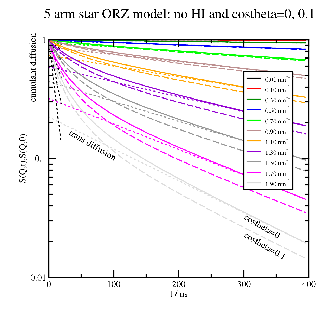
We compare a flexible 10 arm star with a star that has bonds close to the core stretched. We use a simple linear profile while in [1] a two step profile is used.

We observe that the stiff core increases tranlational diffusion (Dcm: 2.1 -> 1.58 nm²/ns) as the star gets larger (Rg: 2.43 -> 3.99 nm). Additional the internal contribution increase in amplitude which might be a result of the increased size as the arms are more extended.

import jscatter as js
import numpy as np

q= np.r_[0.01,0.1:2:0.2]
t = np.r_[0:1:0.02,1:20:1,20:100:5]

p = js.grace()
p.xaxis(label='t / ns')

sqt0 = js.dynamic.multiArmStarORZ(t, q, 10, 50, l=0.5, costheta = 0, reducedfriction=0.2)
for c,sq in enumerate(sqt0,1):
    p.plot(sq.X,sq._Sqt,li=[1,1,c],sy=0,le=f'{sq.q:.2f} nm\\S-1')

# costheta is linear increasing from stretched center to free ends
sqt1 = js.dynamic.multiArmStarORZ(t, q, 5, 50, l=0.5, costheta = np.r_[0.7:0.1:49j], reducedfriction=0.2)
for c,sq in enumerate(sqt1,1):
    p.plot(sq.X,sq._Sqt,li=[3,1,c],sy=0)

p.yaxis(label='S(Q,t),S(Q,0)',scale='log',min=0.01,max=1)
p.legend(charsize=0.7)
p.title('10 arm star ORZ model:')
p.subtitle('solid: costheta=0; broken costheta linear increasing')
p.text('costheta=0',x=300,y=0.031,rot=330)
p.text('costheta=0.1',x=300,y=0.022,rot=330)
# p.save(js.examples.imagepath+'/ORZ_10armStarblob.png',size=(1.5,1.5),dpi=300)

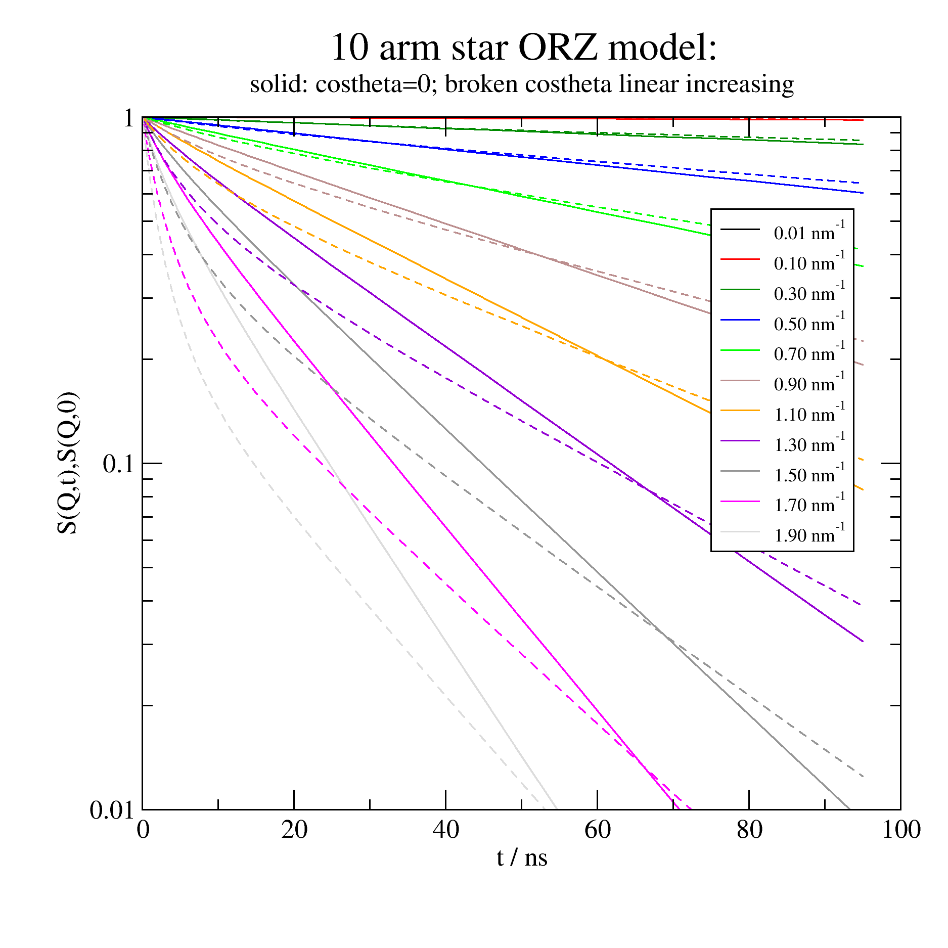
jscatter.dynamic.nSiteJumpDiffusion_w(w, q, N, t0, r0)[source]

Random walk among N equidistant sites (isotropic averaged); dynamic structure factor in w domain.

E.g. for CH3 group rotational jump diffusion over 3 sites.

Parameters:

warray: Frequencies in 1/ns
q: float: Wavevector in units 1/nm
Nint: Number of jump sites, jump angle 2pi/N
r0float: Distance of sites from center of rotation. For CH3 e.g.0.12 nm.
t0float: Rotational correlation time.

Returns:

dataArray

Notes

Equ. 24 [1] :

\[S_{inc}^{rot}(Q,\omega) = B_0(Qa)\delta(\omega) + \frac{1}{\pi} \sum_{n=1}^{N-1} B_n(Qa) \frac{\tau_n}{1+(\omega\tau_n)^2}\]

with $\tau_1=\frac{\tau}{1-cos(2\pi/N)}$ , $\tau_n=\tau_1\frac{sin^2(\pi/N)}{sin^2(n\pi/N)}$

\[B_n(Qa) = \frac{1}{N} \sum_{p=1}^{N} j_0 \Big( 2Qa sin(\frac{\pi p}{N}) \Big) cos(n\frac{2\pi p}{N})\]

References

[1]

Incoherent scattering law for neutron quasi-elastic scattering in liquid crystals. Dianoux, A., Volino, F. & Hervet, H., Mol. Phys. 30, 37–41 (1975). https://doi.org/10.1080/00268977500102721

Examples

import jscatter as js
import numpy as np
w=np.r_[-100:100:0.1]
ql=np.r_[1:14.1:1.3]
p=js.grace()
iqw=js.dL([js.dynamic.nSiteJumpDiffusion_w(w=w,q=q,N=3,t0=0.01,r0=0.12) for q in ql])
p.plot(iqw)
p.yaxis(scale='l',label=r'S(\xw\f{}) / a.u.',min=1e-6,max=1)
p.xaxis(label=r'\xw\f{} / ns\S-1',min=-100,max=100)
# p.save(js.examples.imagepath+'/nSiteJumpDiffusion_w.jpg', size=(2,2))

jscatter.dynamic.resolution(t, s0=1, m0=0, s1=None, m1=None, s2=None, m2=None, s3=None, m3=None, s4=None, m4=None, s5=None, m5=None, s6=None, m6=None, s7=None, m7=None, a0=1, a1=1, a2=1, a3=1, a4=1, a5=1, a6=1, a7=1, bgr=0, resolution=None)[source]

Resolution in time domain as multiple Gaussians for inelastic measurement as back scattering or time of flight instrument.

Multiple Gaussians define the function to describe a resolution measurement. Use `resolution_w` to fit with the appropriate normalized Gaussians and this function to implicit Fourier transform a signal. See Notes.

Parameters:

tarray

Times

s0,s1,…float

Width of Gaussian functions representing a resolution measurement. The number of si not None determines the number of Gaussians.

m0, m1,….float, None

Means of the Gaussian functions representing a resolution measurement.

a0, a1,….float, None

Amplitudes of the Gaussian functions representing a resolution measurement.

bgrfloat, default=0

Background

resolutiondataArray

Resolution with attributes sigmas, amps which are used instead of si, ai.

If resolution is from w domain this represents the Fourier transform from w to t domain. means are NOT used from w domain as these result only in a phase shift, instead m0..m5 are used. If mi is not give zero is assumed.
If from t domain the resolution is recalculated with same parameters for new t.

Returns:

dataArray

Notes

In a typical inelastic experiment the resolution is measured by e.g. a vanadium measurement (elastic scatterer). In t domain (Neutron Spin Echo) this is a carbon black sample for small Q or e.g. Zirconium for higher Q. In w domain the resolution is described by a multi Gaussian function as in resw=resolution_w(w,…) with amplitudes $ai_w$, width $si_w$ and common mean $m_w$.

resolution(t,resolution_w=resw) defines the Fourier transform of resolution_w using the same coefficients as an implicit Fourier transform. $mi_t$ are set by default to zero as $mi_w$ lead only to a phase shift. It is easiest to shift w values in w domain as it corresponds to a shift of the elastic line.

Beside the fitting of resolution measurements the pair of resolution_w and resolution allows a Fourier transform from w to t domain of any signal. If resolution_w is used for fitting of data in the w domain then `ft = resolution(t=..,resolution=resolution_w_fit)` represents the Fourier transform of the fitted data.

The used Gaussians are normalized that they are a pair of Fourier transforms:

\[R_t(t,m_i,s_i,a_i)=\sum_i a_i s_i e^{-\frac{1}{2}s_i^2 t^2} \Leftrightarrow R_w(w,m_i,s_i,a_i)= \sum_i a_i e^{-\frac{1}{2}(\frac{w-m_i}{s_i})^2}\]

under the Fourier transform defined as

\[F(f(t)) = \frac{1}{\sqrt{2\pi}} \int_{-\infty}^{\infty} f(t) e^{-i\omega t} dt\]

\[F(f(w)) = \frac{1}{\sqrt{2\pi}} \int_{-\infty}^{\infty} f(\omega) e^{i\omega t} d\omega\]

Examples

Using the result of a fit in w domain to represent the resolution in time domain :

import jscatter as js
import numpy as np

# resw is a resolution in w domain maybe as a result from a fit to vanadium data
# resw contains all parameters
w = np.r_[-100:100:0.5]
resw = js.dynamic.resolution_w(w, s0=12, m0=0, a0=2)

# representing the Fourier transform of resw as a gaussian transforms to time domain
t = np.r_[0:1:0.01]
rest = js.dynamic.resolution(t,resolution=resw)
t2 = np.r_[0:0.5:0.005]
rest2 = js.dynamic.resolution(t2,resolution=rest)

jscatter.dynamic.resolution_w(w, s0=1, m0=0, s1=None, m1=None, s2=None, m2=None, s3=None, m3=None, s4=None, m4=None, s5=None, m5=None, s6=None, m6=None, s7=None, m7=None, a0=1, a1=1, a2=1, a3=1, a4=1, a5=1, a6=1, a7=1, bgr=0, resolution=None)[source]

Resolution as multiple Gaussians for inelastic measurement as backscattering or time of flight instrument in w domain.

Multiple Gaussians define the function to describe a resolution measurement. Use only a common mi to account for a shift. See resolution() for transform to time domain.

Parameters:

warray

Frequencies

s0,s1,…float

Sigmas of several Gaussian functions representing a resolution measurement. The number of si not none determines the number of Gaussians.

m0, m1,….float, None

Means of the Gaussian functions representing a resolution measurement.

a0, a1,….float, None

Amplitudes of the Gaussian functions representing a resolution measurement.

bgrfloat, default=0

Background

resolutiondataArray

Resolution with attributes sigmas, amps which are used instead of si, ai.

If from t domain this represents the Fourier transform from w to t domain. The means are NOT used from as these result only in a phase shift, instead m0..m5 are used.

If from w domain the resolution is recalculated.

Returns:

dataArray

.means
.amps
.sigmas

Notes

In a typical inelastic experiment the resolution is measured by e.g. a vanadium measurement (elastic scatterer). This is described in w domain by a multi Gaussian function as in resw=resolution_w(w,…) with amplitudes $a_{iw}$, width sigma $s_{iw}$ and common mean $m_w$. To allow asymmetric resolutions as observed on some instruments we use mean $m_{iw}$

resolution(t,resolution_w=resw) defines the Fourier transform of resolution_w using the same coefficients. $m_{it}$ are set by default to 0 (if not explicit set) as $m_{iw}$ lead only to a phase shift. It is easiest to shift w values in w domain as it corresponds to a shift of the elastic line.

The used Gaussians are normalized that they are a pair of Fourier transforms:

\[R_t(t,m_i,s_i,a_i)=\sum_i a_i s_i e^{-\frac{1}{2}s_i^2 t^2} \Leftrightarrow R_w(w,m_i,s_i,a_i)=\sum_i a_i e^{-\frac{1}{2}(\frac{w-m_i}{s_i})^2}\]

under the Fourier transform defined as

\[F(f(t)) = \frac{1}{\sqrt{2\pi}} \int_{-\infty}^{\infty} f(t) e^{-i\omega t} dt\]

\[F(f(w)) = \frac{1}{\sqrt{2\pi}} \int_{-\infty}^{\infty} f(\omega) e^{i\omega t} d\omega\]

Examples

Transform from and to time domain

import jscatter as js
import numpy as np
# resw is a resolution in w domain maybe as a result from a fit to vanadium data
# resw contains all parameters
w=np.r_[-100:100:0.5]
resw=js.dynamic.resolution_w(w, s0=12, m0=0, a0=2)

w2=np.r_[0:50:0.2]
rest2=js.dynamic.resolution_w(w2,resolution=resw)

# representing the Fourier transform of to time domain
t=np.r_[0:1:0.01]
rest=js.dynamic.resolution(t,resolution=resw)

Sequential fit in w domain to a measurement with real data.

The data file is from the SPHERE instrument at MLZ Garching (usually not gzipped). We overfitt the data as we just want a description of Gaussians with $\chi^2 \approx 1$

import jscatter as js
import numpy as np

def readinx(filename,block, l2p):
    # reusable function for inx reading
    # neutron scatterers use strange data formats like .inx dependent on local contact
    # in the beginning we find sometimes an index or the respective Q value or number of channels.
    # here the blocks start with  number of channels. Spaces (' 562 ') are important to find the starting line.
    # this might dependent on instrument and local contact (they can do what you ask for)
    data = js.dL(filename,
                 block=block,                    # this finds the starting of the blocks of all angles or Q
                 usecols=[1,2,3],                # ignore the numbering at each line
                 lines2parameter=l2p)  # catch the parameters at beginning
    for da in data:
        da.channels = da.line_1[0]
        da.Q = da.line_3[0]                       # in 1/A
        da.incident_energy = da.line_3[1]         # in meV
        da.temperature = da.line_3[3]             # in K if given
    return data

vanae = readinx(js.examples.datapath +'/Vana.inx.gz',block=' 562 ',l2p=[-1,-2,-3,-4])

# convert to 1/ns, we can select parts of the data
vanat = js.dynamic.convert_e2w(vanae[:],T=293,unit='μeV')
vana = js.dynamic.shiftAndBinning(vanat)  # if you need the center w0

# low Q might be fitted with less Gaussians
# high Q with 6 Gaussians increasing width , decreasing amplitude
dm = 2
start = {'s0':0.3,'m0':0,'a0':max,'bgr':0.73,
    's1':2,'m1':0,'a1':0.3*max,
    's2':4,'m2':0,'a2':0.1*max,
    's3':8,'m3':0,'a3':0.01*max,
    's4':16,'m4':0,'a4':0.001*max,
    's5':32,'m5':0,'a5':0.0001*max}
for van in vana:
    max= van.Y.max()
    van.setlimit(m0=[-dm,dm],m1=[-dm,dm],m2=[-dm,dm],m3=[-dm,dm],m4=[-dm,dm],m5=[-dm,dm])
    van.setlimit(a0=[0],a1=[0],a2=[0],a3=[0],a4=[0],a5=[0])
    van.setlimit(s0=[0],s1=[0],s2=[0],s3=[0],s4=[0],s5=[0])
    van.makeErrPlot(yscale='log', fitlinecolor=11,title=f'Q={van.Q:.3f}')
    van.fit(js.dynamic.resolution_w,start,{},{'w':'X'},
                     max_nfev=20000,method='lm',diff_step=0.001,workers=0)
    van.lastfit.Q = van.Q  # needed later
    start = van.getFreepar  # use last result as new start parameter

# save to recover later (that we dont need to repeat this)
vanalastfit = js.dL([v.lastfit for v in vana])
vanalastfit.save('Vana_fitted.inx.gz')

Recover the result to use for convolution in a later step

# recover by
vanalastfit = js.dL('Vana_fitted.inx.gz')
vanalastfit.getfromcomment('modelname')

# select a specific Q and recalculate; w can also be adopted to be different
vanQ = vanalastfit.filter(Q=1.417)[0]
res = js.dynamic.resolution_w(w=vanQ.X, resolution=vanQ)

# vana[6].showlastErrPlot(yscale='log',fitlinecolor=6,title=f'Q={vana[7].Q:.3f}')
# vana[6].savelastErrPlot(js.examples.imagepath+'/resolutionfit.jpg')

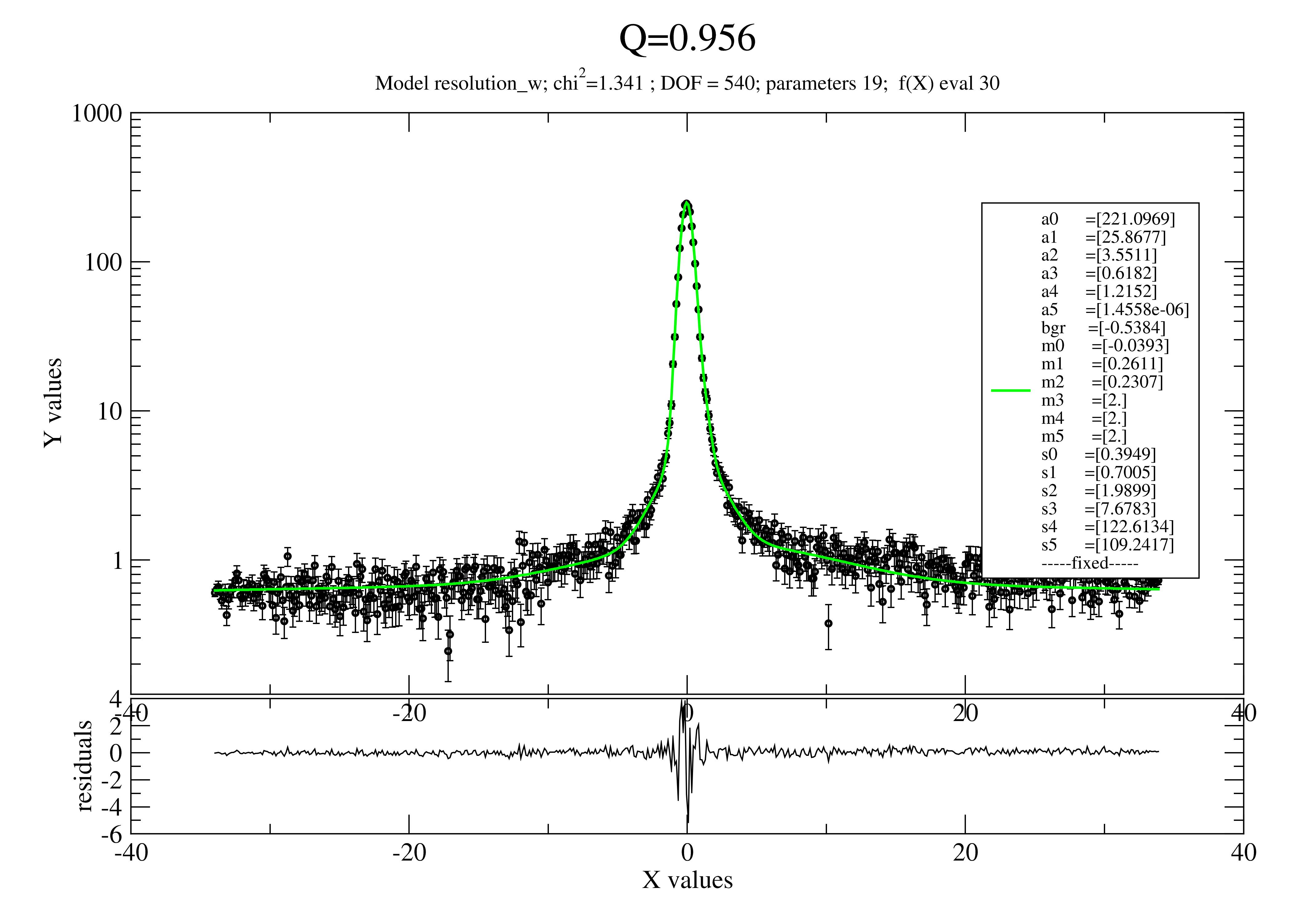
jscatter.dynamic.ringChainORZ(t, q, N=100, l=1, fa=None, Dcm=None, Dcmfkt=None, viscosity=1, T=293, reducedfriction=0.25, tintern=0)[source]

Dynamics of a ring polymer using optimized Rouse-Zimm approximation (ORZ).

The ring dynamic structure factor is calculated in analogy to the star described by Guenza [1].

The ring chain dynamics is decribed within the more general optimized Rouse-Zimm (ORZ) approximation introduced by Bixon and Zwanzig [3] [4] . See solveOptimizedRouseZimm().

We extend this here using bead scattering lengths for partial matching and allow individual bond correlations.

To speedup fitting use the memoize function as described in memoize().

Parameters:

tarray

timepoints in units ns.

qarray

Scattering vectors in units 1/nm.

Nint

Number of beads .

lfloat, default = 0.38 nm (amino acid)

Bond length or Kuhn length in units nm.

faNone, list of float

Scattering length of bead/monomer $fa_i$. Can be used to match parts of the star to the solvent.

None : Equal 1 for all beads.
list: length N as scattering length of beads in sequence

Dcmfloat

Center of mass diffusion in units nm**2/ns. If None the calculated value D_ORZ is used.

Dcmfktarray 2xN, function

Function f(q) or array with [qi, f(qi) ] as correction for Dcm like Diff = Dcm*f(q). e.g. for inclusion of structure factor or hydrodynamic function with f(q)=H(Q)/S(q). Missing values are interpolated.

viscosityfloat, default=1 (H2O@20C )

$\eta$ in units cPoise=mPa*s e.g. water $visc(T=293 K) =1 mPas$

Tfloat, default 273+20

Temperature in Kelvin.

reducedfrictionfloat, default 0.25

Reduced friction $\zeta_r = \zeta/6\pi\eta_sl$ in hydrodynamic tensor H.

=0 : free draining limit, no HI, Rouse dynamics.
>0 : with HI typically <0.5. For h>0.5 we get negative eigenvalues.

See solveOptimizedRouseZimm().

During fits use limits(reducedfriction=[0,0.43,0.,0.5]) to avoid singular matrices.

tinternfloat>0, default 0

Relaxation time due to internal friction between neighboring beads in ns.

Returns:

sqtdataList

Intermediate scattering function of a star for given q.

[times; Sqt; Sqt only diffusion; Sqt cumulant]
columnname = ‘t;Sqt;Sqt_inf;Sqt_cum’
.q : scattering vector
.D_ORZcum : diffusion coefficinet in initial slope (cumulant)
.D_ORZ : translational diffusion ORZ model
.Dcm : used center of friction/mass diffusion
.Fq : form factor
.Fq_inf : form factor t=inf
.beadfriction : bead friction
.bondrateconstant : bondrateconstant in 1/ns
.moderelaxationtimes : used moderelaxationtimes in ns [4] equ 2.17
.mode_rmsd : used mode rmsd as math:`l/mu^{0.5} # [4] equ 2.19
.reducedfriction : reducedfriction
.eigenvalues : all evals
.mu : all mu
.l : bondlength l
.N : Number of beads
.Rg : radius of gyration in nm
.Rg_red : reduced radius of gyration

Notes

See solveOptimizedRouseZimm() for a description of the ORZ model with respective parameters and the dynamic structure factor $S(q,t)/S(q,0)$ .

Here we use a ring chain with N beads of uncorelated beads with costheta=0 .

The structural matrix has diagonal elements, $A_{ii}=2$ and $A_{i\neq j}=-1$ if the ith and jth monomers are connected to each other or zero otherwise.

References

[1]

Static and Dynamic Structure Factors for Star Polymers in θ Conditions. Guenza, M. & Perico, A. Macromolecules 26, 4196–4202 (1993). https://doi.org/10.1021/ma00068a020

[2]

A Local Approach to the Dynamics of Star Polymers. Guenza, M., Mormino, M. & Perico, A. Macromolecules 24, 6168–6174 (1991). https://doi.org/10.1021/ma00023a018

[3]

Theoretical basis for the Rouse‐Zimm model in polymer solution dynamics. Zwanzig, R. The Journal of Chemical Physics 60, 2717–2720 (1974) https://doi.org/10.1063/1.1681433

[4]

A hierarchy of models for the dynamics of polymer chains in dilute solution. Perico, A., Ganazzoli, F. & Allegra, G. The Journal of Chemical Physics 87, 3677–3686 (1987). https://doi.org/10.1063/1.452966

[5]

Rubinstein, M. & Colby, R. H. Polymer Physics. (OUP Oxford, 2003).

[6]

Intramolecular relaxation dynamics in semiflexible dendrimers. Kumar, A. & Biswas, P. Journal of Chemical Physics 134, (2011). https://doi.org/10.1063/1.3598336

Examples

Here we examine how HI changes dynamics.

import jscatter as js
import numpy as np

q= np.r_[0.01,0.1:2:0.2]
t = np.r_[0:1:0.02,1:20:1,20:100:5]

p = js.grace()
p.xaxis(label='t / ns')

sqt = js.dynamic.ringChainORZ(t, q, 100, l=0.5, reducedfriction=0)
for c,sq in enumerate(sqt,1):
    p.plot(sq.X,sq._Sqt,li=[1,1,c],sy=0,le=f'{sq.q:.2f} nm\\S-1')

sqt = js.dynamic.ringChainORZ(t, q, 100, l=0.5, reducedfriction=0.05)
for c,sq in enumerate(sqt,1):
    p.plot(sq.X,sq._Sqt,li=[3,1,c],sy=0,le='')

p.yaxis(label='S(Q,t),S(Q,0)',scale='log',min=0.1,max=1)
p.legend(charsize=0.7)
p.title('rings with and without HI ')
p.subtitle('solid: no HI; broken: with HI')

# p.save(js.examples.imagepath+'/ORZ_ringHI.png',size=(1.5,1.5),dpi=300)

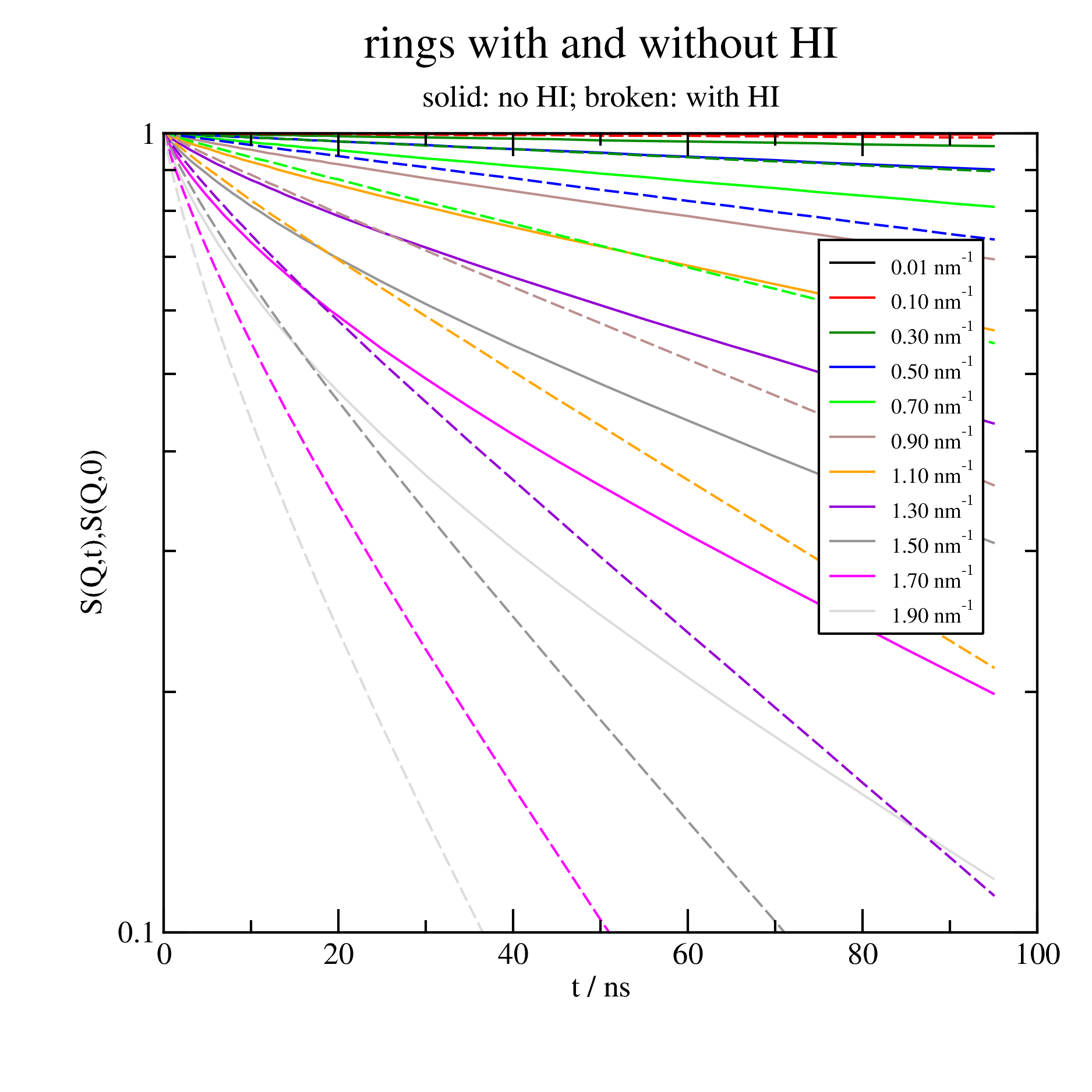
jscatter.dynamic.rotDiffusion_w(w, q, cloud, Dr, lmax='auto')[source]

Rotational diffusion of an object (dummy atoms); dynamic structure factor in w domain.

A cloud of dummy atoms can be used for coarse graining of a non-spherical object e.g. for amino acids in proteins. On the other hand its just a way to integrate over an object e.g. a sphere or ellipsoid. We use [2] for an objekt of arbitrary shape modified for incoherent scattering.

Parameters:

warray

Frequencies in 1/ns

qfloat

Wavevector in units 1/nm

cloudarray Nx3, Nx4 or Nx5 or float

A cloud of N dummy atoms with positions cloud[:3] that describe an object.
If given, cloud[3] is the incoherent scattering length $b_{inc}$ otherwise its equal 1.
If given, cloud[4] is the coherent scattering length otherwise its equal 1.
If cloud is single float the value is used as radius of a sphere with 10x10x10 grid.

Drfloat

Rotational diffusion constant in units 1/ns.

lmaxint

Maximum order of spherical bessel function. ‘auto’ -> lmax > 2pi*r.max()*q/6.

Returns:

dataArray: Columns [w; Iqwinc; Iqwcoh] Input parameters as attributes.

Notes

See transRotDiffusion() for more details. The Fourier transform of the exp function is a Lorentzian so the exp should be changed to a Lorentzian.

References

[1]

Incoherent scattering law for neutron quasi-elastic scattering in liquid crystals. Dianoux, A., Volino, F. & Hervet, H. Mol. Phys. 30, 37–41 (1975).

[2]

Effect of rotational diffusion on quasielastic light scattering from fractal colloid aggregates. Lindsay, H., Klein, R., Weitz, D., Lin, M. & Meakin, P. Phys. Rev. A 38, 2614–2626 (1988).

Examples

import jscatter as js
import numpy as np
R=2;NN=10
Drot=js.formel.Drot(R)
ql=np.r_[0.5,2:18.:3]
w=np.r_[-100:100:0.1]
grid=js.ff.superball(ql,R,p=1,nGrid=NN,returngrid=True)
p=js.grace()
iqwR1=js.dL([js.dynamic.rotDiffusion_w(w,q,grid.XYZ,Drot) for q in ql])
p.plot(iqwR1,le=f'NN={NN:.0f} q=$wavevector nm\S-1')
p.yaxis(scale='l',label=r'S(\xw\f{}) / a.u.',min=1e-4,max=1e4)
p.xaxis(label=r'\xw\f{} / ns\S-1',min=-100,max=100)
p.legend(x=30,y=9000,charsize=0.8)
# p.save(js.examples.imagepath+'/transRotDiffusion_w.jpg', size=(2,2))

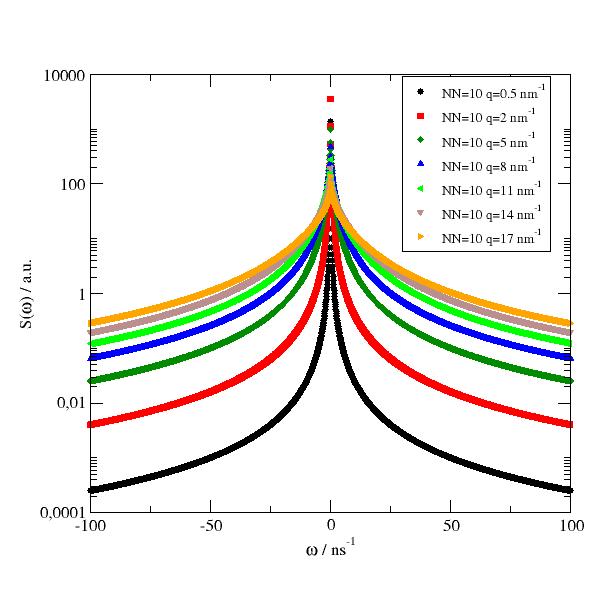
jscatter.dynamic.shiftAndBinning(data, w=None, w0=None, Qname='Q')[source]

Shift w spectrum and average (binning) in intervals.

The intention is to shift and average over intervals in frequency space. - Shift models to data.

For model results it should be used after convolution with the instrument resolution, when singular values at zero are smeared by resolution. Binning is like detector average.

Experimental data peaks can be shifted to zero. Binning including error bars is liek average over several detectors.

Parameters:

datadataArray, dataList

Data to be shifted and averaged.

warray

New X values (e.g. from experiment) after shifting to w0. .Y values are averaged over both side half intervalls around new values.

If w is None original is used values are used.

If zeros in eY no weight is applied (equal weight).

w0float, dataList default None

Shift by w0 that w_new = w_old - w0

If shifted by resolution with w0 attribute the w0 from resolution measurement is used at correct Q.
If w0 is None the center of intensity between lower and upper FWHM is used e.g. for resolution measurement.

Qnamestring, default ‘Q’

Attribute name of the scattering vector.

Returns:

resultdataArray

.w0 is original center of peak as center of intensity between FWHM.

Examples

See also frequency2timeFF()

import jscatter as js
import numpy as np

w = np.r_[-100:100:0.5]
start = {'s0':6,'m0':0,'a0':1,'s1':None,'m1':0,'a1':1,'bgr':0.00}
resolution = js.dynamic.resolution_w(w,**start)

p = js.grace(1,0.6)
p.plot(resolution, le='original')

wnew = np.r_[-100:100:1.5]
p.plot(js.dynamic.shiftAndBinning(resolution,w=wnew,w0=20),le='explicit w0')
p.plot(js.dynamic.shiftAndBinning(resolution,w=wnew,w0=None),le='find w0')

p.legend()
p.yaxis(label='S(w) / a.u.')
p.xaxis(label=r'w / ns\S-1')
# p.save(js.examples.imagepath+'/shiftAndBinning.jpg', size=(2,2))

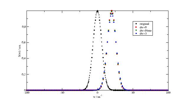
jscatter.dynamic.simpleDiffusion(t, gamma=None, q=None, D=None, s=0, beta=1, type='lognorm')[source]

Intermediate scattering function [g1(t)] for diffusing particles from distribution of relaxation rates.

\[I(q,t,D, \sigma ) = \beta \int g(\Gamma, \Gamma_0, \sigma ) e^{-\Gamma t}\]

and relaxation rate $\Gamma_0=q^2D$.

Parameters:

tfloat, array

Times

gammafloat

Mean relaxation rate in inverse t units. Overrides q and D if given. If q and D given gamma=q*q*D

qfloat, array

Wavevector

betafloat

Intercept $\beta$ in DLS. The amplitude prefactor.

Dfloat

Mean diffusion coefficient.

sfloat

Relative standard deviation of the diffusion coefficient distribution from e.g. polydispersity. In absolute units $\sigma=s*q^2*D=w\Gamma$. For a typical DLS experiment s≈0.25 just from instrument noise (e.g. noise ≈ 1e-3 Zetasizer Nano, Malvern)

For s=0 a single exponential is used.

type‘truncnorm’, default ‘lognorm’

Distribution shape.

‘lognorm’ lognorm istribution as normal distribution on a log scale.

\[g(x, \m, \sigma) = \frac{ 1 }{\ x\sigma\sqrt{2\pi}} exp(-\frac{\ln(x- \mu)^2}{ 2 \sigma^2 })\]

This is approximatly what you get from CONTIN or NNLS algorithm in DLS.
‘truncnorm’ normaldistribution cut at zero.

\[g(x, \mu, \sigma)= e^{-0.5(\frac{x-\mu}{\sigma})^2} / (\sigma\sqrt{2\pi}) \ \text{ for x>0}\]

Returns:

outdataArray

intermediate scattering function or $g_1$

.D, .wavevector, .beta respective input parameters
pdf : Probability of the distribution in the interval around pdf[0,i] (half distance to neighboring points) that sum(pdf[2])==1 similar to CONTIN results.

Notes

Units of q, t and D result in unit-less [q*q*D*t] like q in 1/cm, t in s -> D in cm*cm/s .

Remember that $g_2(t)$ (intensity correlation for DLS) is $g_1^2(t)=g_2(t)-1$.

Examples

import jscatter as js
import numpy as np

t = js.loglist(1e-6,10,1000) # in seconds

# ≈ a protein with a MW of 140kDa
D = 3e-7  # unit cm^2/s
q = 4*np.pi/633e-7*np.sin(np.pi/4)  # 90º HeNe laser in DLS

p=js.grace(1.8,1)
p.multi(1,2)
p[0].xaxis(label=r't / s ',scale='log')
p[0].yaxis(label=r'g\s1\N(t) ')
p[1].xaxis(label=r'\xG\f{} / 1/s ',scale='log')
p[1].yaxis(label=[r'P(\xG\f{})',1,'opposite'],)

for c,s in enumerate([0.25,0.5,1,2],1):
   dls = js.dynamic.simpleDiffusion(t=t,q=q,D=D,s=s)
   p[0].plot(dls,sy=0,li=[1,3,c],le=f's={s}')
   p[1].plot(dls.pdf[0], 20 * dls.pdf[1],sy=0,li=[1,3,c])

p[0].legend(x=0.01,y=0.8)
p[0].title('DLS correlation')
p[1].title('rate distribution')
# p.save(js.examples.imagepath+'/simpleDiffusion.jpg',size=(1.8,1))

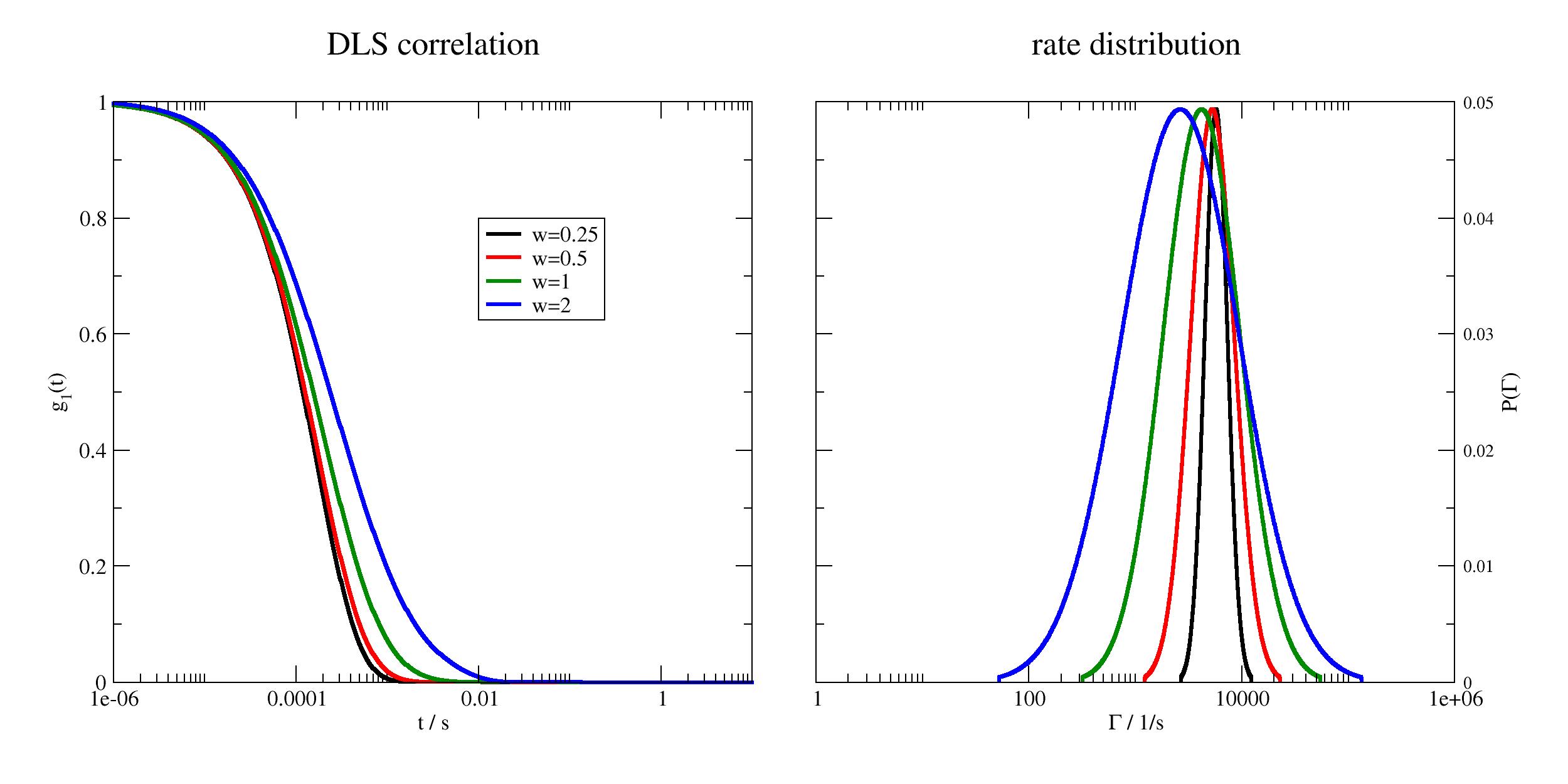
jscatter.dynamic.solveOptimizedRouseZimm(A, reducedfriction=0.25)[source]

Solve optimized Rouse-Zimm (ORZ) approximation to the diffusion equation of a polymer in solution.

From [1] : A generalization of some work by Bixon on the theoretical foundations of the Rouse-Zimm model in polymer solution dynamics. In particular, a procedure is described for constructing the “best possible” Rouse-Zimm model for an arbitrary polymer, starting from the equilibrium distribution of polymer conformations and using either Kirkwood’s generalized diffusion dynamics or stochastic dynamics. The method is based on an application of linear response theory to the calculation of certain time correlation functions for polymer dynamics.

Parameters:

A[N,N] array

Structural matrix.

reducedfrictionfloat

Reduced friction $\zeta_r= \zeta/6\pi\eta_s l$ in matrix of the preaveraged hydrodynamic interactions $H_{ij}=\delta_{ij} + \zeta_r \langle l/R_{ij}\rangle (1-\delta_{ij})$. The default 0.25 is in accordance with experimental data for theta solvents [2].

=0 : free draining limit, no HI, Rouse dynamics. H is identity matrix that $HA=A$.

>0 : with HI typically <0.5. For h>0.5 we may get negative eigenvalues.

[3] : The value of $\zeta_r = 0.25$ ensures that the matrix [H] is positive definite and does not show any instabilities related to the appearance of negative unphysical eigenvalues. Such eigenvalues occur when the parameter $\zeta_r$ exceeds a critical value $\zeta_r^*$ which corresponds to the non-overlapping condition $r/b=\frac{bead radius}{bond length} ≤ 0.5$ for the monomers.

[6] : The abrupt change in $\phi_{max}$ at r/b~O.43 indicates that a large perturbation takes place in the modes. Therefore, this value has to be considered an upper limit to the strength of the hydrodynamic interaction. More restrictive conditions, physically reasonable though arbitrary, fall in the range of r/b lower than 0.43 but do not apparently give rise to anomalies in the modes. In the application to intrinsic viscosity in ideal solvents, presented in Sec. III, we shall therefore take r/b in the range 0-0.40.

Returns:

evalHA, evecHA, A, loverR, Rg2_red, Rij2_redarray’s

evalHA1D array: Eigenvalues $\lambda_a$ of $HA$.
evecHA2D array: Eigenvectors $Q_{ia}$ of $HA$.
mu1D array: Diagonal elements $\mu_a = (Q^TAQ)_{aa}$
loverR2D array: Adimensional mean inverse distance matrix equ. 25 in [4] : $\langle l/R_{ij}\rangle =l(6/\pi)^{1/2}(\langle R^2_{ij}\rangle )^{-1/2}$ .
Rg2_redfloat: Reduced radius of gyration (equ 3.2 in [2]) $R_g^2/l^2 = \sum_{ij} \langle R^2_{ij}\rangle / (2N^2)$
Rij2_red2D array: Reduced second moments for the distance between any two chain atoms equ. 3.1 in [2] :

\[\langle R^2_{ij}\rangle /l^2= \sum_{k=1}^{N} (Q_{ik} - Q_{jk})^2/\lambda_k\]
A2D array: Dimesionless structural matrix $A = M[1:,:].T * U * M[1:,:]$ (or force constant matrix as $3kT/l^2 A$ or connectivity matrix)

Notes

In the ORZ approximation to the Kirkwood configurational diffusion equation, the bead coordinates of a chain of N beads (or monomers) of friction coefficient $\zeta$ jointed by equal links of mean square length $l^2$ and forceconstant $\kappa$ obey a Langevin equation of the form

\[\begin{split}\zeta \frac{\partial}{\partial t} R_i(t) + \kappa \sum_{j} (HA)_{ij} R_j(t) = v_i(t) \\ \frac{\partial}{\partial t} R_i(t) + \sigma \sum_{j} (HA)_{ij} R_j(t) = v_i(t)\end{split}\]

were $v_i$ is the random velocity, $\sigma=\kappa/\zeta=3kT/l^2\zeta$ as bond rate constant [4] and bead coordinates $R_i$. $\zeta=6\pi\eta_0l$ is the bead friction with the surrounding/solvent.

The structural matrix $A$ depends on the actual shape of the polymer (e.g. linear, star or ring).

The matrix H is the preaveraged hydrodynamic matrix with elements

\[H_{ij} = \delta_{ij} + \zeta_r\langle l/R_{ij}\rangle (1-\delta_{ij})\]

with $R_{ij}$ as distance between beads i and j, reduced friction per chain atom $\zeta_r=\zeta/6\pi\eta_0l$ and $\eta_0$ as solvent viscosity.

The structural matrix A of a linear polymer is

\[\begin{split}A = M^T \left( \begin{array}{cc} 0 & 0 \\ 0 & U \end{array} \right) M = M[1:,:]^T U M[1:,:]\end{split}\]

with the transfer matrix M in dimsionless form (the first row is not needed)

\[\begin{split}M = \left ( \begin{array}{cccc} 1/N & 1/N & ... & 1/N \\ -1 & 1 & 0 & 0..0 \\ 0 & -1 & 1 & 0..0 \\ ... \end{array} \right )\end{split}\]

In the first dimension is the center of mass that is basically not needed.

Elements of $M_{ij}$ are −1 if the bond vector $l_i$ starts at monomer i and +1 if bond vector $l_i$ points to bead i, else 0.

U can be retrieved from (depends on the model: freely jointed chain (FJC), free rotating chain (FRC), RIS,…)

\[U^{-1}_{ij} = \langle l_i\cdot l_j\rangle /l^2\]

Freely jointed linear chain and bead spring model:

\[\langle l_i\cdot l_j\rangle /l^2 = \delta_{ij} \Rightarrow \langle R^2_{ij}\rangle = l^2 |i-j|\]
Free rotating linear chain with bond angles $g=-cos(\theta)$ ($\theta=\pi$ is rigid rod)

\[\langle l_i\cdot l_j\rangle/l^2 = g^{|i-j|} \Rightarrow \langle R^2_{ij}\rangle = l^2 |i-j| [\frac{1+g}{1-g} -\frac{2g}{|i-j|}\frac{1-g^{|i-j|}}{(1-g)^2}]\]

Persistence length is $nl=l/(1-g)$ and $\langle R^2_{ij}\rangle$ from [5]. For $g=0$ we yield the FJC.

The solution of a ORZ model can be described by normal modes and corresponding eigenvalues $Q_a, \lambda_a$ of the matrix $HA$ yielding normal coordinates $\Xi_k$, mode relaxation times $\tau_a$ and mean square displacements $\langle \xi^2_a \rangle$ and

\[\xi_k(t) = Q_{ki} R_i(t)\]

\[\tau_a=(\sigma \lambda_a)^{-1}\]

\[\langle \xi^2_a\rangle = l^2 \mu_a^{-1}\]

where $\mu_a= (Q^TAQ)_{aa}$. For free draining ($\zeta_r=0$) $\mu_a=\lambda_a$

According to the usual Zimm notation, the mode $a=0$ describes the translational mode of the center of resistance, always characterized by a constant eigenvector $Q_{k,0} = N^{-1/2}$ and a zero relaxation rate $\lambda_0 = 0$

The dynamic correlation between beads i and j is [1] :

\[\begin{split}\langle |R_i(t) -R_j(0)|^2\rangle &= l^2 \sum_{a=1}^{N-1} \mu_a^{-1} [|Q_{ia}|^2+|Q_{ja}|^2 - (Q_{ia}Q_{ka}^* + Q_{ia}Q_{ka}^*) exp(-\sigma\lambda_at)] \\ &= l^2 \sum_{a=1}^N \mu_a^{-1} [|Q_{ia}|^2+|Q_{ja}|^2 - 2Q_{ia}Q_{ka} exp(-\sigma\lambda_at)] \\ &= l^2 d_{ij}^2\end{split}\]

where the first refers to complex eigenvectors [2] and the later to real eigenvectors [4].

The dynamic structure factor (measured by DLS or NSE) is [4] (here extended by bead scattering amplitudes $f_{i}$):

\[\begin{split}S(q,t)/S(q,0) &= \frac{1}{F(q)} \sum_{ij}^{N} f_{i}f_{j} exp(-q^2/6\langle |R_i(t) -R_j(0)|^2\rangle ) \\ &= \frac{1}{F(q)} exp(-q^2Dt) \sum_{ij}^{N} f_{i}f_{j }exp(-q^2l^2/6 \cdot d_{ij}^2)\end{split}\]

with the form factor $F(q)$ and (equ. 8 in [4])

\[d_{ij}^2 = \sum_{a=1}^N \mu_a^{-1} [|Q_{ia}|^2+|Q_{ja}|^2 - 2Q_{ia}Q_{ka} exp(-\sigma\lambda_at))]\]

Note

One should recognize the similarity in the description to normal modes of biomacromolecules reprectively proteins as described in the Ornstein-Uhlenbeck process jscatter.bio.intScatFuncOU(). The difference is the explicit usage of coordinates in jscatter.bio.intScatFuncOU() while in the ORZ model statistical averages of $d_{ij}$ without explicit coordinates are used.

We yield the static form factor as for $t \rightarrow 0$

\[\begin{split}F(Q) &= S(q,0) =& \sum_{ij}^N f_{i}f_{j}exp(-\frac{q^2}{6}\langle R_{ij}^2\rangle ) \\ \hat{F}(Q) &= & \frac{1}{N^2}\sum_{ij}^N exp(-\frac{q^2}{6}\langle R_{ij}^2\rangle )\end{split}\]

where the second line is the normalized form factor equ. 2 in [4] with $f_i=1$.

The translational diffusion coefficient is equ. 24 in [4]:

\[D = kT/N\zeta [1 + \frac{\zeta_r}{N}\sum_{ij} (1-\delta_{ij}) \langle l/R_{ij}\rangle ]\]

The first cumulant observed in an experiment at short times (initial slope $\Omega(q)=-(d/dt)ln(S(q,t))|_{t=0}=\Omega(q)$) is equ. 13 in [4] for $f_i=1$:

\[\Omega(q) = q^2D_{cum} = q^2 \frac{\sigma l^2}{3N} \frac{1}{\hat{F}(q)} [1 + \frac{\zeta_r}{N} \sum_{ij} (1-\delta_{ij}) \langle l/R_{ij}\rangle exp(-q^2l^2/6 \cdot d_{ij}^2(0) )]\]

The prefactor is $\sigma l^2/(3N)=kT/N\zeta$ as in the equation above.

Taking into account the scattering amplitudes $f_i$ we yield with the NOT normalized form factor $F(q)$

\[\Omega(q) = q^2 D_{cum} = q^2 \frac{\sigma l^2}{3} \frac{1}{F(q)F(0)} [\sum_{i=j}f_i^2 + \sum_{i\neq j} f_i f_j \zeta_r \langle l/R_{ij}\rangle exp(-q^2l^2/6 \cdot d_{ij}^2(0) )]\]

Here we see that specific bead/arm contributions can be suppressed if the respective beads are matched to the surrounding solvent. Nevertheless, the overall tranlational diffusion will not change by matching.

The dynamic intrinsic viscosity can be calculated from the relaxation times equ. 21 in [5] :

\[[\eta(\omega)] = \frac{N_akT}{M\eta_0} \sum_{a} \frac{\tau_a}{1+i\omega\tau_a}\]

with M as molecular weight and $N_a$ as Avogadro constant.

Note

It should be pointed out that the matrix $U^{-1}$ geht highly singular if the model is applied to more rigid chains or rodlike parts resulting in negative eigenvalues.

Internal friction

Internal friction $\zeta_{int}$ between neigboring beads can be included in analogy to Soranno [7]

\[\zeta \frac{\partial}{\partial t} R_i(t) + \kappa \sum_{j} (HA)_{ij} R_j(t) + \zeta_{int} \frac{\partial}{\partial t} (HA)_{ij} R_j(t) = v_i(t)\]

with the additional friction term. Using the above eigenvectors of $HA$ this leads to

\[\begin{split}\zeta \frac{\partial}{\partial t} \xi_k(t) + \kappa \lambda_k \xi_k(t) + \zeta_{int} \frac{\partial}{\partial t} \lambda_k \xi_k(t) &= w_k(t) \\ [(\zeta +\zeta_{int} \lambda_k)\frac{\partial}{\partial t}\xi_k(t) = - \kappa \lambda_k \xi_k(t) + w_k(t)\end{split}\]

and result in same eigenvectors but changed relaxation times $\tau_{a,int}=(\sigma \lambda_a)^{-1} + \tau_{int} = \tau_a + \tau_{int}$ with $\tau_{int} = \zeta_{int}/\kappa$ as presented by Sorrano for standard Rouse/Zimm model [7]. The additional internal friction is here independent of the modes and has a stronger effect on higher modes.

In above corrrelation functions we need to change

\[\begin{split}&exp(-\sigma\lambda_a t)=exp(- \frac{t}{\tau_a}) \rightarrow \\ &exp(-\frac{\sigma \lambda_a}{1+\sigma \lambda_a \tau_{int}}t)=exp(-\frac{t}{\tau_a+\tau_{int}})\end{split}\]

Here $\tau_a$ contains implicitly the mode dependence $\tau_{zp}=\tau_zp^{-3\nu}$ for Zimm or $\tau_{rp}=\tau_zp^{-2}$ for Rouse like systems (see finiteRouse(), finiteZimm()) but the additional mode independent internal friction is the same. Correspondingly in the cumulant a correction is needed $\langle l/R_{ij}\rangle \rightarrow \langle l/R_{ij}\rangle \sum_a 1/(1+\sigma\lambda_a \tau_{int})$

References

[1] (1,2)

Theoretical basis for the Rouse‐Zimm model in polymer solution dynamics. Zwanzig, R. The Journal of Chemical Physics 60, 2717–2720 (1974) https://doi.org/10.1063/1.1681433

[2] (1,2,3,4,5)

A hierarchy of models for the dynamics of polymer chains in dilute solution. Perico, A., Ganazzoli, F. & Allegra, G. The Journal of Chemical Physics 87, 3677–3686 (1987). https://doi.org/10.1063/1.452966

[3]

Intramolecular relaxation dynamics in semiflexible dendrimers. Kumar, A. & Biswas, P. Journal of Chemical Physics 134, (2011). https://doi.org/10.1063/1.3598336

[4] (1,2,3,4,5,6)

Static and Dynamic Structure Factors for Star Polymers in θ Conditions. Guenza, M. & Perico, A. Macromolecules 26, 4196–4202 (1993). https://doi.org/10.1021/ma00068a020

[5] (1,2)

Optimized Rouse–Zimm theory for stiff polymers M. Bixon; R. Zwanzig J. Chem. Phys. 68, 1896–1902 (1978) https://doi.org/10.1063/1.435916

[6] (1,2,3)

Dynamics of chain molecules. I. Solutions to the hydrodynamic equation and intrinsic viscosity. Perico, A., Piaggio, P. & Cuniberti, C. The Journal of Chemical Physics 62, 4911–4918 (1975). https://doi.org/10.1063/1.430404

[7] (1,2)

Internal friction in an intrinsically disordered protein - Comparing Rouse-like models with experiments A. Soranno, F. Zosel, H. Hofmann J. Chem. Phys. 148, 123326 (2018) http://aip.scitation.org/doi/10.1063/1.5009286

Examples

Example to reproduce Fig 6 of [2] (only left subplot) but in simpler model (not RIS) just using bead-spring (FJC) and free rotating chain models for linear polymers:

Non-vanishing bond correlations increase size. Draining increases relaxation times but not the msd of the movements.

import jscatter as js
import numpy as np

p = js.grace(1.9,1.)
p.multi(1,3,hgap=0.25)
p[0].yaxis(label=r'\xl\f{}\sa')
p[1].yaxis(label=r'\xt\f{}\sa\N\xs',scale='log',ticklabel=['power',0])
p[2].yaxis(label=r'\x<z\f{}\S2\N\sa\N>/l\S2',scale='log',ticklabel=['power',0])
p[0].xaxis(label=r'a')
p[1].xaxis(label=r'a',scale='log')
p[2].xaxis(label=r'a',scale='log')

# matrices for linear chain
N=100
M = np.diag([1.]*(N+1)) +  np.diag([-1.]*N,-1)
U = np.diag([1.]*N)
A = M[1:,:].T @ U @ M[1:,:]
ev, evec, mu = js.dynamic.solveOptimizedRouseZimm(A, reducedfriction=0.25)[:3]
a = np.r_[1:ev.shape[0]]
p[0].plot(a, ev[1:],le='FJC partial draining')
p[1].plot(a, 1/ev[1:],le='FJC partial draining')
p[2].plot(a, 1/mu[1:],le='FJC partial draining')

ev, evec, mu = js.dynamic.solveOptimizedRouseZimm(A, reducedfriction=0)[:3]
a = np.r_[1:ev.shape[0]]
p[0].plot(a, ev[1:],le='FJC free draining')
p[1].plot(a, 1/ev[1:],le='FJC free draining')
p[2].plot(a, 1/mu[1:],le='FJC free draining')

# matrices for linear chain but non-vanishing bond correlation
costheta = 0.65
i,j = np.indices([N,N])
Uinv = costheta**np.abs(i-j)
U = np.linalg.inv(Uinv)
A = M[1:,:].T @ U @ M[1:,:]
ev, evec, mu = js.dynamic.solveOptimizedRouseZimm(A, reducedfriction=0.25)[:3]
a = np.r_[1:ev.shape[0]]
p[0].plot(a, ev[1:],le='FRC partial draining')
p[1].plot(a, 1/ev[1:],le='FRC partial draining')
p[2].plot(a, 1/mu[1:],le='FRC partial draining')

ev, evec, mu = js.dynamic.solveOptimizedRouseZimm(A, reducedfriction=0)[:3]
a = np.r_[1:ev.shape[0]]
p[0].plot(a, ev[1:],le='FRC free draining')
p[1].plot(a, 1/ev[1:],le='FRC free draining')
p[2].plot(a, 1/mu[1:],le='FRC free draining')

p[0].subtitle('eigenvalue spectra')
p[1].subtitle('relaxation times')
p[2].subtitle('mean square displacements')
p[1].title('model FJC + FRC free draining and partial draining')
p[1].legend(x=1.4,y=1,charsize=0.8)
# p.save(js.examples.imagepath+'/ORZeigenvalue.jpg',size=(1.9,1.),dpi=200)

Correctness of the solution can be verified by comparing to Table I of [6]. The parameter h in [6] corresponds to reducedfriction $=r/b= (\pi/(3N))^{1/2}h \approx 0.1023 h$

Today the eigenvalue problem can be solved directly and is more accurate.

import jscatter as js
import numpy as np

# matrices for linear chain
N=100
M = np.diag([1.]*(N+1)) +  np.diag([-1.]*N,-1)
U = np.diag([1.]*N)
A = M[1:,:].T @ U @ M[1:,:]
# for h=1 or 2 compare to :math:`\lambda_k` (second and 4th column) and :math:`\mu_k` for h=0 to exact solution.
ev, evec, mu = js.dynamic.solveOptimizedRouseZimm(A, reducedfriction=0.2)[:3]
ev[-1]  # ~ 2.66
mu[-1]  # ~ 3.99
ev, evec, mu = js.dynamic.solveOptimizedRouseZimm(A, reducedfriction=0.1)[:3]
ev[-1]  # ~ 3.33
mu[-1]  # ~ 3.99

jscatter.dynamic.stretchedExp(t, gamma, beta, amp=1)[source]

Stretched exponential function.

\[I(t) = amp\, e^{-(t\gamma)^\beta}\]

Parameters:

tarray: Times
gammafloat: Relaxation rate in units 1/[unit t]
betafloat: Stretched exponent
ampfloat default 1: Amplitude

Returns:

dataArray

jscatter.dynamic.stretchedExp_beta05_w(w, gamma)[source]

KWW in frequency domain as analytic Fourier tranform of stretched exponential with beta=0.5.

Same as Kohlrausch–Williams–Watts (KWW) in frequency domain as Fourier tranform of stretched exponential with beta=1. We use here the normalized form $\int_{-\infty}^{\infty} \tilde{\phi}(\omega) = 1$

Parameters:

wfloat or array-like: Frequency
gammafloat: Relaxation rate $\gamma$ in units 1/[unit t] with characteristic time $\tau=1/\gamma$ .

Returns:

float or ndarray, always >= 0

Notes

Analytical derivation of the cosine Fourier transform of the Kohlrausch–Williams–Watts (KWW) stretched exponential with $\beta = 1/2$, expressed in closed form via Fresnel integrals.

The solution can be found in [deGennes19] equ. 11. We write here in a normalized form $\int_{-\infty}^{\infty} \tilde{\phi}(\omega) = 1$ Below the derivation is given with missing prefactor $\frac{1}{\pi}$ :

\[\tilde{\phi}(\omega) = \frac{1}{\pi} \sqrt{\frac{\pi}{2\omega^3\tau}} \left[ \left(\tfrac{1}{2} - S(\theta)\right)\sin\theta + \left(\tfrac{1}{2} - C(\theta)\right)\cos\theta \right], \qquad \theta = \frac{1}{4|\omega|\tau}.\]

Valid for all real $\omega$. The function is even in $\omega$, non-negative, and satisfies:

$\tilde{\phi}(0) = 2\tau/\pi$ (mean relaxation time)
$\tilde{\phi}(\omega) \propto \omega^{-1/2}$ as $\omega\tau \to \infty$

Note the elegant structure: $C$ and $S$ are both evaluated at $\theta$, the same argument as $\sin\theta$ and $\cos\theta$.

Fresnel Integral Convention

The Fresnel integrals are defined here as (analog to ref 8 in [deGennes19])

\[C(x) = \sqrt{\frac{2}{\pi}}\int_0^{\sqrt{x}} \cos(t^2)\,\mathrm{d}t, \qquad S(x) = \sqrt{\frac{2}{\pi}}\int_0^{\sqrt{x}} \sin(t^2)\,\mathrm{d}t,\]

with common limit

\[C(\infty) = S(\infty) = \tfrac{1}{2}.\]

Relation to the SciPy convention scipy.special.fresnel() (denoted $C_s$, $S_s$, which use $\cos(\pi t^2/2)$):

\[C(x) = C_s\!\left(\sqrt{\tfrac{2x}{\pi}}\right), \qquad S(x) = S_s\!\left(\sqrt{\tfrac{2x}{\pi}}\right).\]

The Kohlrausch–Williams–Watts (KWW) stretched exponential is

\[\phi(t) = \exp\!\left[-\left(\frac{t}{\tau}\right)^{\!\beta}\right], \qquad t \geq 0,\]

where $\tau > 0$ is the characteristic time and $\beta = 1/2$. The mean relaxation time (first relaxation time) is

\[\langle\tau\rangle = \int_0^\infty \phi(t)\,\mathrm{d}t = \frac{\tau}{\beta}\,\Gamma\!\left(\frac{1}{\beta}\right) \;\xrightarrow{\;\beta=1/2\;}\; 2\tau.\]

The cosine Fourier transform convention used here is

\[\tilde{\phi}(\omega) = \int_0^\infty \cos(\omega t)\,\phi(t)\,\mathrm{d}t.\]

Derivation

Step 1 — Substitution $s=\sqrt{t}$

Set $s = \sqrt{t}$, so $t = s^2$, $\mathrm{d}t = 2s\,\mathrm{d}s$ and $\phi(t) = e^{-s/\sqrt{\tau}}$:

\[\tilde{\phi}(\omega) = 2\int_0^\infty s\,\cos(\omega s^2)\,e^{-s/\sqrt{\tau}}\,\mathrm{d}s.\]

Step 2 — Integration by Parts

Using $\tfrac{\mathrm{d}}{\mathrm{d}s}\sin(\omega s^2) = 2\omega s\cos(\omega s^2)$, the boundary term vanishes and

\[\tilde{\phi}(\omega) = \frac{1}{\omega\sqrt{\tau}} \underbrace{ \int_0^\infty \sin(\omega s^2)\,e^{-s/\sqrt{\tau}}\,\mathrm{d}s }_{K(\omega,\,\tau)}.\]

Step 3 — Reduction to a Laplace–Fresnel Integral

Substitute $t = s\sqrt{\omega}$, so $\omega s^2 = t^2$ and $s/\sqrt{\tau} = \beta t$ with

\[\beta = \frac{1}{\sqrt{\omega\tau}}.\]

Then $K = (1/\sqrt{\omega})\,\mathrm{Im}\,G(\beta)$, giving

(1)\[\tilde{\phi}(\omega) = \frac{\mathrm{Im}\,G(\beta)}{\omega^{3/2}\sqrt{\tau}}, \qquad G(\beta) = \int_0^\infty e^{it^2 - \beta t}\,\mathrm{d}t.\]

Step 4 — Contour Evaluation of $G(\beta)$

Complete the square in the exponent,

\[it^2 - \beta t = i\!\left(t + \tfrac{i\beta}{2}\right)^{\!2} + \tfrac{i\beta^2}{4},\]

and substitute $v = t + i\beta/2$. The path of $v$ is a horizontal line at height $\mathrm{Im}(v) = \beta/2$. Since $|e^{iv^2}| = e^{-2\,\mathrm{Re}(v)\,\mathrm{Im}(v)} \to 0$ as $\mathrm{Re}(v) \to \infty$, Cauchy’s theorem allows deformation to the real axis:

\[G(\beta) = e^{i\beta^2/4} \left[ \int_0^\infty e^{iv^2}\,\mathrm{d}v - \int_0^{i\beta/2} e^{iv^2}\,\mathrm{d}v \right].\]

The first integral equals $C(\infty) + iS(\infty) = (1+i)/2$. For the imaginary-axis segment, parametrise $v = iy$ with $y: 0 \to \beta/2$, $\mathrm{d}v = i\,\mathrm{d}y$:

\[\int_0^{i\beta/2} e^{iv^2}\,\mathrm{d}v = i\int_0^{\beta/2} e^{-iy^2}\,\mathrm{d}y = S\!\left(\tfrac{\beta}{2}\right) + i\,C\!\left(\tfrac{\beta}{2}\right).\]

Since $\beta/2 = \sqrt{\theta}$ where $\theta \equiv \beta^2/4$, the Fresnel integrals with argument $\beta/2$ are related to those with argument $\theta$ by

\[\int_0^{\beta/2} \cos(t^2)\,\mathrm{d}t = \sqrt{\tfrac{\pi}{2}}\,C(\theta), \qquad \int_0^{\beta/2} \sin(t^2)\,\mathrm{d}t = \sqrt{\tfrac{\pi}{2}}\,S(\theta).\]

Assembling all pieces:

\[G(\beta) = e^{i\theta} \left[ \left(\tfrac{1}{2} - S(\theta)\right) + i\left(\tfrac{1}{2} - C(\theta)\right) \right].\]

Final Result in not normalized form

Taking $\mathrm{Im}\,G(\beta)$ and inserting into (1):

\[\tilde{\phi}(\omega) = \sqrt{\frac{\pi}{2\omega^3\tau}} \left[ \left(\tfrac{1}{2} - S(\theta)\right)\sin\theta + \left(\tfrac{1}{2} - C(\theta)\right)\cos\theta \right], \qquad \theta = \frac{1}{4|\omega|\tau}.\]

Valid for all real $\omega$. The function is even in $\omega$, non-negative, and satisfies:

$\tilde{\phi}(0) = 2\tau$ (mean relaxation time)
$\tilde{\phi}(\omega) \propto \omega^{-1/2}$ as $\omega\tau \to \infty$

Note the elegant structure: $C$ and $S$ are both evaluated at $\theta$, the same argument as $\sin\theta$ and $\cos\theta$.

Asymptotic Limits

Low frequency: $\omega\tau \ll 1$

As $\omega \to 0$, $\theta \to \infty$ and $C(\theta), S(\theta) \to 1/2$, so both bracket terms vanish. The prefactor $\omega^{-3/2}$ is compensated and one recovers

\[\tilde{\phi}(\omega) \;\xrightarrow{\;\omega\tau \to 0\;}\; 2\tau.\]

High frequency: $\omega\tau \gg 1$

As $\omega \to \infty$, $\theta \to 0$, $C(\theta) \approx S(\theta) \approx 0$, $\cos\theta \to 1$, $\sin\theta \to 0$, so

\[\tilde{\phi}(\omega) \;\xrightarrow{\;\omega\tau \to \infty\;}\; \frac{1}{2}\sqrt{\frac{\pi\tau}{\omega}} \;\propto\; \omega^{-1/2}.\]

This $\omega^{-1/2}$ power law is the hallmark of Rouse-mode dynamics and arises naturally because $\beta = 1/2$ is produced by Fresnel-type integrals over Gaussian chain modes (de Gennes, 1979).

References

[KWW1854]

R. Kohlrausch, Theorie des elektrischen Rückstandes in der Leidener Flasche, Ann. Phys. Chem. 91, 179 (1854).

[WW1970]

G. Williams and D. C. Watts, Non-symmetrical dielectric relaxation behaviour arising from a simple empirical decay function, Trans. Faraday Soc. 66, 80 (1970).

[deGennes1979]

P.-G. de Gennes, Scaling Concepts in Polymer Physics, Cornell University Press, Ithaca (1979).

[AS1972]

M. Abramowitz and I. A. Stegun, Handbook of Mathematical Functions, Dover, New York (1972), Chap. 7.

[deGennes19] (1,2)

Quasi-Elastic Scattering of Neutrons by Dilute Polymer Solutions: I. Free-Draining Limit. de Gennes, P.-G. Physics Physique Fizika 1967, 3 (1), 37–45. https://doi.org/10.1103/PhysicsPhysiqueFizika.3.37.

jscatter.dynamic.stretchedExp_w(w, gamma, beta, tfactor=7)[source]

KWW in frequency domain as Fourier tranform of stretched exponential.

\[I(\omega) = FFT(I(t)) = FFT(e^{-(t\gamma)^\beta}) \text{ with normalization} \int_{-\infty}^{\infty} I(\omega) = 1\]

Parameters:

warray: Frequencies in 1/ns
gammafloat: Relaxation rate in units 1/[unit t]
betafloat: Stretched exponent
tfactorfloat: Power factor ``2**tfactor``to expand time range and time steps in FFT to improve accuracy.

Returns:

dataArray

Examples

import jscatter as js
import numpy as np

w = np.r_[-80:80:0.1]
p = js.grace()
g=2

sqw1 = js.dynamic.stretchedExp_w(w, gamma=g, beta=1)
sqwL = js.dynamic.lorentz_w(w, hwhm = g)

maxerr = (np.abs(sqw1.Y-sqwL.Y)/sqwL.Y).max()
p.plot(sqw1,sy=[1,0.4,1],le=fr'stretched beta=1 max rel err :{maxerr:.4g}')
p.plot(sqwL,sy=0,li=[1,1,11],le='Lorentz analytic')

sqw05 = js.dynamic.stretchedExp_w(w, gamma=g, beta=0.5,tfactor=23)
sqw05a = js.dynamic.stretchedExp_beta05_w(w,g)

maxerr = (np.abs(sqw05.Y-sqw05a.Y)/sqw05a.Y).max()
p.plot(sqw05,sy=[1,0.4,2],le=fr'stretched beta=0.5 max rel err :{maxerr:.4g}')
p.plot(sqw05a,sy=0,li=[1,1,5],le='stretched beta=0.5 analytic')

p.yaxis(label='S(w)',scale='log',min=1e-4,max=1)
p.xaxis(label='w / 1/ns',scale='norm',min=-80,max=80)
p.legend(x=15,y=sqw05.Y.max(),charsize=0.7)
p.title('Comparison FFT(stretched exp.) to analytic result')

# p.save(js.examples.imagepath+'/stretchedExp_w.png',size=(1.5,1.5),dpi=300)

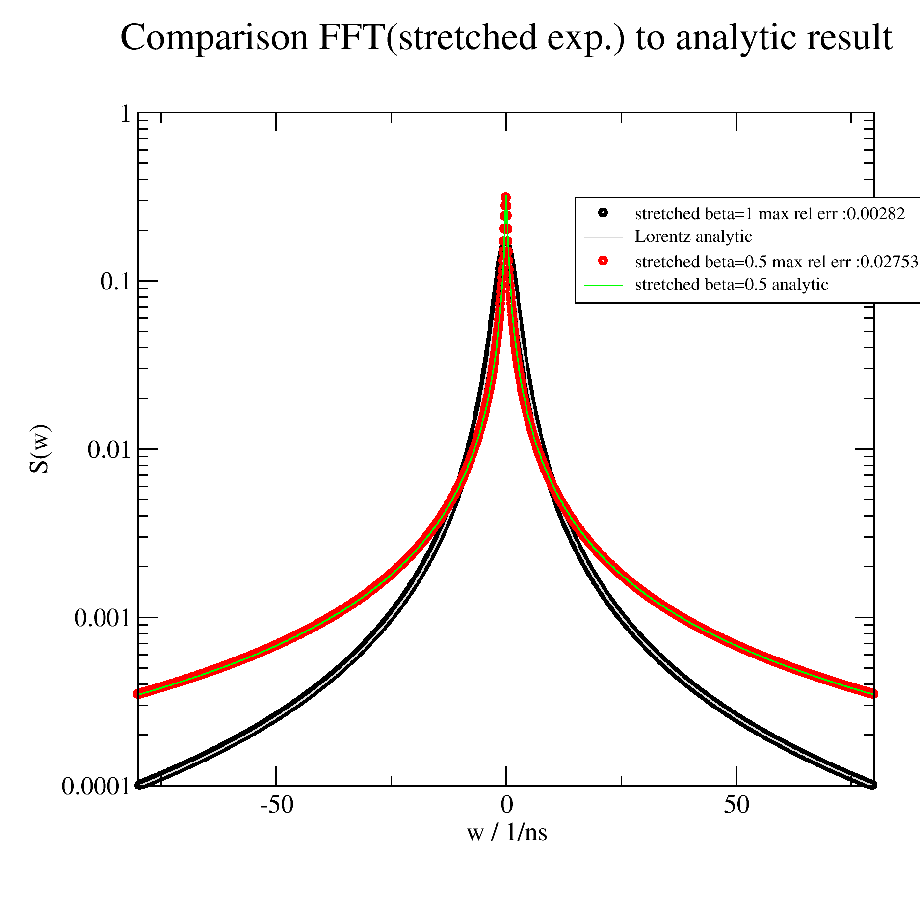
jscatter.dynamic.threeLorentz_w(w, Q, g1, a1, resolution, g2=1, a2=0, g3=1, a3=0, a0=0, bgr=0, u2=0, wmax=None)[source]

Three Lorents functions with elastic contribution and resolution smearing.

A convenience function that allows to directly fit experimental data.

Parameters:

warray

Frequencies 1/ns

Qfloat

Wavevector in 1/nm for selecting the correct resolution.

g1,g2, g3float

FWHM units 1/ns.

a1,a2,a3float

Amplitudes of the Lorentz functions.

a0float

Amplitude elastic contribution. If the resolution is normalized it is directly the elastic contribution.

resolutiondataList

Measured or calculated resolution function with same Q as in the data to fit.

Normalize the resolution before usage that the elastic amplitude a0 gets meaningful.
In general it is assumed that the resolution and data w are equidistant.
A fitted resolution can be used to smooth noise in a measured resolution. See resolution_w() how to fit and use the ‘.lastfit’ .

bgrfloat

Background.

u2float , default=0

Means square displacement $\langle u^2\rangle$ for the Debye-Waller factor in 1/Q**2 units. Only useful if several Q are fitted simultaneous.

The used Debye-Waller factor is $DWF(Q,\langle u^2\rangle) = exp(-Q^2\langle u^2\rangle /3)$

wmaxfloat, default None

Cutoff frequency for resolution. Not needed for fitted resolution.

Returns:

modeldataArray: Q : wavevector

Notes

We sum here three Lorentz functions with amplitudes and add an elastic contribution. For Lorentz see lorentz_w() that are convoluted with the resolution cut at wmax. As elastic contribution we use the given resolution cut at wmax and multiplied by value elastic.

For independent process j the inelastic measurement is often expressed by an elastic and an inelastic term as

\[S_j(Q,\omega) \propto [B_{0j}(Q)\delta(Q) + (1-B_{0j}(Q)) L_j(Q,\omega)] \otimes R(Q,\omega)\]

with the resolution function $R(Q, \omega)$ and the Lorentzian

\[L_j(Q,\omega) = \frac{1}{\pi} \frac{\Gamma_j(Q)}{\omega^2+\Gamma^2_j(Q)}\]

For several processes the summed intensity including a Debye-Waller factor is

\[\begin{split}I(Q,\omega) = [ exp(-Q^2\langle u^2\rangle) \big( &A_0(Q)\delta(Q) + \\ \sum_j &A_j(Q) L_j(Q,\omega) \big) ] \otimes R(Q,\omega)\end{split}\]

where the elastic contributions are summed in a single term $A_{0}(Q)\delta(Q)$

Examples

import jscatter as js
import numpy as np

def readEMUdat(filename, wavelength=6.27084, temperature=0):
    # Read data form EMU@ANSTO as direct output from Mantid (No .inx converison needed)
    data = js.dL(filename, delimiter=',')
    for da in data:
        da.Q = np.round(float(da.comment[0]),4)
        da.temperature = temperature
        da.wavelength = wavelength
    # cut the zero at the end
    for i in range(len(data)):
        data[i] = data[i,:,:-1]
    return data

vanae = readEMUdat(js.examples.datapath + '/sample_5K_Q.dat.gz', temperature=5)
vana = js.dynamic.convert_e2w(vanae, 0, unit='meV')
# convert resolution to normalized data that elastic has meaning
for va in vana:
    va.integral = np.trapezoid(va.Y,va.X)
    va.Y = va.Y/va.integral  # normalise resolution
    va.eY = va.eY/va.integral  # normalise resolution

# read new data and convert to 1/ns
same = readEMUdat(js.examples.datapath + '/sample_413K_Q.dat.gz',temperature=413)
sam = js.dynamic.convert_e2w(same, 293, unit='meV')

# Fit one after the other
for n in np.r_[0:len(sam)]:
    #sam[n].makeErrPlot(yscale='log', title=str(sam[1].Q) + ' A\S-1')
    sam[n].setlimit()  # removes limits
    sam[n].setlimit(a0=[0, 1], bgr=[0., 0.01])
    sam[n].setlimit(a1=[0],a2=[0],a3=[0])  # no negative amplitudes
    sam[n].setlimit(g1=[0,100],g2=[0,100],g3=[0,100])  # no negative and some max
    sam[n].fit(js.dynamic.threeLorentz_w,
        {'a0': 1, 'bgr': 1e-5, 'a1': 0.2,'g1':16,'a2': 0.2,'g2':6,   },
        {'wmax':8, 'a3':0,'g3': 1,'resolution':vana},
        {'w': 'X'},
        method='lm',max_nfev=20000)
    #sam[n].killErrPlot()  # close it , or uncomment to have them open

# look at one single errplot
n=3
sam[n].showlastErrPlot(title=str(sam[n].Q) , yscale='log')
sam[n].errPlot(sam[n].lastfit.X,sam[n].lastfit._lo1,sy=0,li=[1,2,3],le='lo 1')  # add
sam[n].errPlot(sam[n].lastfit.X,sam[n].lastfit._lo2,sy=0,li=[1,2,4],le='lo 2')
sam[n].errPlot(sam[n].lastfit.X,sam[n].lastfit._lo3,sy=0,li=[1,2,6],le='lo 3')
sam[n].errPlot(sam[n].lastfit.X,sam[n].lastfit._el,sy=0,li=[1,2,5],le='elastic')

# sam[n].errplot.save(js.examples.imagepath+'/threeLorentz_w.jpg', size=(2,2))

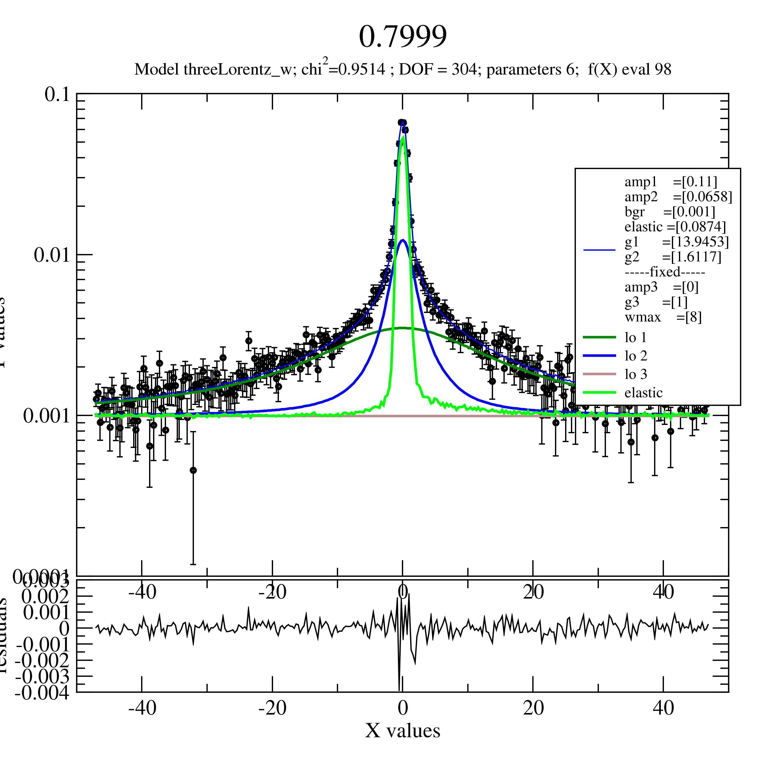
jscatter.dynamic.time2frequencyFF(timemodel, resolution, w=None, tfactor=7, **kwargs)[source]

Fast Fourier transform from time domain to frequency domain for inelastic neutron scattering.

Shortcut t2fFF calls this function.

Parameters:

timemodelfunction, None

Model for I(t,q) in time domain. t in units of ns. The values for t are determined from w as $t=[0..n_{max}]\Delta t$ with $\Delta t=1/max(|w|)$ and $n_{max}=w_{max}/\sigma_{min} tfactor$. $\sigma_{min}$ is the minimal width of the Gaussians given in resolution. If None a constant function (elastic scattering) is used.

resolutiondataArray, float

dataArray : dataArray that describes the resolution function as multiple Gaussians.

Use resolution_w() for fitting the resolution measurement. A nonzero bgr in resolution is ignored.
float : Gives the width of a single Gaussian in units 1/ns (w is needed below).

Resolution width is in the range of 6 1/ns (IN5 TOF) to 1 1/ns (Spheres BS).
anything else: no resolution.

warray

Frequencies for the result, e.g. from experimental data. If w is None the frequencies resolution.X are used. This allows to use the fit of a resolution to be used with same w values.

kwargskeyword args

Additional keyword arguments that are passed to timemodel.

tfactorfloat, default 7

Factor to determine max time for timemodel to minimize spectral leakage. tmax=1/(min(resolution_width)*tfactor) determines the resolution to decay as $e^{-tfactor^2/2}$. The time step is dt=1/max(|w|). A minimum of len(w) steps is used (which might increase tmax). Increase tfactor if artifacts (wobbling) from the limited time window are visible as the limited time interval acts like a window function (box) for the Fourier transform.

Returns:

dataArrayA symmetric spectrum of the Fourier transform is returned.

.Sq $\rightarrow S(q)=\int_{-\omega_{min}}^{\omega_{max}} S(Q,\omega)d\omega \approx \int_{-\infty}^{\infty} S(Q,\omega)d\omega = I(q,t=0)$

Integration is done by a cubic spline in w domain on the ‘raw’ fourier transform of timemodel.

.Iqt timemodel(t,kwargs) dataArray as returned from timemodel.

Implicitly this is the Fourier transform to time domain after a successful fit in w domain. Using a heuristic model in time domain as multiple Gaussians or stretched exponential allows a convenient transform to time domain of experimental data.

Notes

We use Fourier transform with real signals. The transform is defined as

\[F(f(t)) = \frac{1}{\sqrt{2\pi}} \int_{-\infty}^{\infty} f(t) e^{-i\omega t} dt\]

\[F(f(w)) = \frac{1}{\sqrt{2\pi}} \int_{-\infty}^{\infty} f(\omega) e^{i\omega t} d\omega\]

The resolution function is defined as (see resolution_w)

\[ \begin{align}\begin{aligned}\begin{split}R_w(w,m_i,s_i,a_i)&= \sum_i a_i e^{-\frac{1}{2}(\frac{w-m_i}{s_i})^2} = F(R_t(t)) \\\end{split}\\&=\frac{1}{\sqrt{2\pi}} \int_{-\infty}^{\infty} \sum_i{a_i s_i e^{-\frac{1}{2}s_i^2t^2}} e^{-i\omega t} dt\end{aligned}\end{align} \]

using the resolution in time domain with same coefficients $R_t(t,m_i,s_i,a_i)=\sum_i a_i s_i e^{-\frac{1}{2}s_i^2 t^2}$

The Fourier transform of a timemodel I(q,t) is

\[I(q,w) = \frac{1}{\sqrt{2\pi}} \int_{-\infty}^{\infty} I(q,t) e^{-i\omega t} dt\]

The integral is calculated by Fast Fourier transform as

\[I(q,m\Delta w) = \frac{1}{\sqrt{2\pi}} \Delta t \sum_{n=-N}^{N} I(q,n\Delta t) e^{-i mn/N}\]

$t_{max}=tfactor/min(s_i)$. Due to the cutoff at $t_{max}$ a wobbling might appear indicating spectral leakage. Spectral leakage results from the cutoff, which can be described as multiplication with a box function. The corresponding Fourier Transform of the box is a sinc function visible in the frequency spectrum as wobbling. If the resolution is included in time domain, it acts like a window function to reduce spectral leakage with vanishing values at $t_{max}=N\Delta t$. The second possibility (default) is to increase $t_{max}$ (increase tfactor) to make the sinc sharp and with low wobbling amplitude.

Mixed domain models

Associativity and Convolution theorem allow to mix models from frequency domain and time domain. After transformation to frequency domain the w domain models have to be convoluted with the FFT transformed model.

Examples

Other usage example with a comparison of w domain and transformed from time domain can be found in A comparison of different dynamic models in frequency domain or in the example of diffusionHarmonicPotential_w().

Compare transDiffusion transform from time domain with direct convolution in w domain.

import jscatter as js
import numpy as np
w=np.r_[-100:100:0.5]
start={'s0':6,'m0':0,'a0':1,'s1':None,'m1':0,'a1':1,'bgr':0.00}
resolution=js.dynamic.resolution_w(w,**start)

p=js.grace(1,1)
D=0.035;qq=3  # diffusion coefficient of protein alcohol dehydrogenase (140 kDa) is 0.035 nm**2/ns
p.title('Inelastic spectrum IN5 like')
p.subtitle(r'resolution width about 6 ns\S-1\N, Q=%.2g nm\S-1\N' %(qq))

# compare diffusion with convolution and transform from time domain
diff_ffw=js.dynamic.time2frequencyFF(js.dynamic.simpleDiffusion,resolution,q=qq,D=D)
diff_w=js.dynamic.transDiff_w(w, q=qq, D=D)
p.plot(diff_w,sy=0,li=[1,3,3],le=r'diffusion D=%.3g nm\S2\N/ns' %(D))
p.plot(diff_ffw,sy=[2,0.3,2],le='fft from time domain')
p.plot(diff_ffw.X,diff_ffw.Y+diff_ffw.Y.max()*1e-3,sy=[2,0.3,7],le=r'fft from time domain with bgr')

# resolution has to be normalized in convolve
diff_cw=js.dynamic.convolve(diff_w,resolution,normB=1)
p.plot(diff_cw,sy=0,li=[1,3,4],le='after convolution in w domain')
p.plot(resolution.X,resolution.Y/resolution.integral,sy=0,li=[1,1,1],le='resolution')

p.yaxis(min=1e-6,max=5,scale='l',label='S(Q,w)')
p.xaxis(min=-100,max=100,label=r'w / ns\S-1')
p.legend(x=10,y=4)
p.text(string=r'convolution edge ==>\nmake broader and cut',x=10,y=8e-6)
# p.save(js.examples.imagepath+'/dynamic_t2f_examples.jpg', size=(2,2))

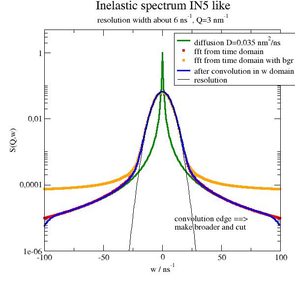
Compare the resolutions direct and from transform from time domain.

p=js.grace()
fwres=js.dynamic.time2frequencyFF(None,resolution)
p.plot(fwres,le='fft only resolution')
p.plot(resolution,sy=0,li=2,le='original resolution')

Compare diffusionHarmonicPotential to show simple usage

import jscatter as js
import numpy as np
t2f=js.dynamic.time2frequencyFF
dHP=js.dynamic.diffusionHarmonicPotential
w=np.r_[-100:100]
ql=np.r_[1:14.1:6j]
iqw=js.dL([js.dynamic.diffusionHarmonicPotential_w(w=w,q=q,tau=0.14,rmsd=0.34,ndim=3) for q in ql])
# To move spectral leakage out of our window we increase w and interpolate.
# The needed factor (here 23) depends on the quality of your data and background contribution.
iqt=js.dL([t2f(dHP,'elastic',w=w*13,q=q, rmsd=0.34, tau=0.14 ,ndim=3,tfactor=14).interpolate(w) for q in ql])

p=js.grace()
p.multi(2,3)
p[1].title('Comparison direct and FFT  for ndim= 3')
for i,(iw,it) in enumerate(zip(iqw,iqt)):
    p[i].plot(iw,li=1,sy=0,le='q=$wavevector nm\S-1')
    p[i].plot(it,li=2,sy=0)
    p[i].yaxis(min=1e-5,max=2,scale='log')
    if i in [1,2,4,5]:p[i].yaxis(ticklabel=0)
    p[i].legend(x=5,y=1, charsize=0.7)

jscatter.dynamic.transDiff(t, q, D)[source]

Translational diffusion intermediate scattering function in t domain.

\[I(t,q) = e^{-q^2Dt}\]

Parameters:

tarray: Frequencies in 1/ns
qfloat: Wavevector in nm**-1
Dfloat: Diffusion constant in nm**2/ns

Returns:

dataArray

jscatter.dynamic.transDiff_w(w, q, D)[source]

Translational diffusion; dynamic structure factor in w domain.

Parameters:

warray: Frequencies in 1/ns
qfloat: Wavevector in nm**-1
Dfloat: Diffusion constant in nm**2/ns

Returns:

dataArray

Notes

Equ 33 in [1]

\[I(\omega,q) = \frac{1}{\pi} \frac{Dq^2}{(Dq^2)^2 + \omega^2}\]

References

[1]

Scattering of Slow Neutrons by a Liquid Vineyard G Physical Review 1958 vol: 110 (5) pp: 999-1010

Examples

import jscatter as js
import numpy as np
ql = np.r_[0.5,2:18.:3]
w = np.r_[-100:100:0.1]
p = js.grace()
iqwD = js.dL([js.dynamic.transDiff_w(w,q,0.02) for q in ql])
p.plot(iqwD,le=f'q=$wavevector nm\S-1')

p.yaxis(scale='l',label=r'S(\xw\f{}) / a.u.',min=1e-7,max=100)
p.xaxis(label=r'\xw\f{} / ns\S-1',min=-100,max=100)
p.legend(x=30,y=100,charsize=0.8)
# p.save(js.examples.imagepath+'/transDiff_w.jpg', size=(2,2))

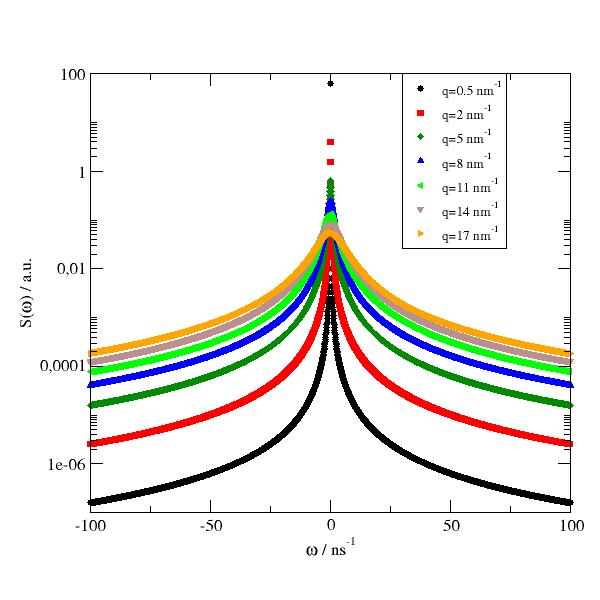
jscatter.dynamic.transRotDiffusion(t, q, cloud, Dr, Dt=0, lmax='auto')[source]

Translational + rotational diffusion of an object (dummy atoms); dynamic structure factor in time domain.

A cloud of dummy atoms can be used for coarse graining of a non-spherical object e.g. for amino acids in proteins. On the other hand its just a way to integrate over an object e.g. a sphere or ellipsoid (see example). We use [2] for an objekt of arbitrary shape modified for incoherent scattering.

Parameters:

tarray

Times in ns.

qfloat

Wavevector in units 1/nm

cloudarray Nx3, Nx4 or Nx5 or float

A cloud of N dummy atoms with positions cloud[:3] in units nm that describe an object .
If given, cloud[3] is the incoherent scattering length $b_{inc}$ otherwise its equal 1.
If given, cloud[4] is the coherent scattering length $b_{coh}$ otherwise its equal 1.
If cloud is single float the value is used as radius of a sphere with 10x10x10 grid points.

Drfloat

Rotational diffusion constant (scalar) in units 1/ns.

Dtfloat, default=0

Translational diffusion constant (scalar) in units nm²/ns.

lmaxint

Maximum order of spherical bessel function. ‘auto’ -> lmax > 2π r.max()*q/6.

Returns:

dataArray

Columns [t; Iqtinc; Iqtcoh; Iqttrans]

.radiusOfGyration
.Iq_coh coherent scattering (formfactor)
.Iq_inc incoherent scattering
.wavevector
.rotDiffusion
.transDiffusion
.lmax

Notes

We calculate the field autocorrelation function given in equ 24 in [2] for an arbitrary rigid object without additional internal dynamic as

\[I(q,t) = e^{-q^2D_tt} I_{rot}(q,t) = e^{-q^2D_tt} \sum_l S_{l,i/c}(q)e^{-l(l+1)D_rt}\]

where $I_{rot}(q,t)$ is the rotational diffusion contribution and

\[ \begin{align}\begin{aligned}\begin{split}S_{l,c}(q) &= 4\pi \sum_m |\sum_i b_{i,coh} j_l(qr_i) Y_{l,m}(\Omega_i)|^2 & coherent scattering \\\end{split}\\\begin{split}S_{l,i}(q) &= \sum_m \sum_i (2l+1) b_{i,inc}^2 |j_l(qr_i)|^2 & incoherent scattering\\\end{split}\end{aligned}\end{align} \]

and coh/inc scattering length $b_{i,coh/inc}$, position vector $r_i$ and orientation of atoms $\Omega_i$, spherical Bessel function $j_l(x)$, spherical harmonics $Y_{l,m}(\Omega_i)$.

The incoherent intermediate scattering function is res.Y/res.Iq_inc or res._Iqtinc/res.Iq_inc
The coherent intermediate scattering function is res._Iqtcoh/res.Iq_coh
For real scattering data as backscattering or spinecho coherent and incoherent have to be mixed according to the polarisation conditions of the experiment accounting also for spin flip probability of coherent and incoherent scattering. For the simple case of non-polarised measurement we get

\[I(q,t)/I(q,0) = \frac{I_{coh}(q,t)+I_{inc}(q,t)}{I_{coh}(q,0)+I_{inc}(q,0)}\]

References

[1]

Incoherent scattering law for neutron quasi-elastic scattering in liquid crystals. Dianoux, A., Volino, F. & Hervet, H. Mol. Phys. 30, 37–41 (1975).

[2] (1,2)

Effect of rotational diffusion on quasielastic light scattering from fractal colloid aggregates. Lindsay, H., Klein, R., Weitz, D., Lin, M. & Meakin, P. Phys. Rev. A 38, 2614–2626 (1988).

Examples

A bit artificial look at only rotational diffusion of a superball build from dummy atoms. (rotational diffusion should only show if also translational diffusion is seen) Change p to change from spherical shape (p=1) to cube (p>10) or star like (p<0.5) (use grid.show() to take a look at the shape) The coherent contribution is suppressed for low q if the particle is spherical .

import jscatter as js
import numpy as np
R=2;NN=10
ql=np.r_[0.4:2.:0.3,2.1:15:2]
t=js.loglist(0.001,50,50)
# get superball
p2=1
grid=js.ff.superball(ql,R,p=p2,nGrid=NN,returngrid=True)
Drot=js.formel.Drot(R)
Dtrans=js.formel.Dtrans(R)
p=js.grace(1.5,1)
p.new_graph(xmin=0.23,xmax=0.43,ymin=0.25,ymax=0.55)
iqt=js.dL([js.dynamic.transRotDiffusion(t,q,grid.XYZ,Drot,lmax=30) for q in ql])

for i,iiqt in enumerate(iqt,1):
    p[0].plot(iiqt.X,iiqt.Y/iiqt.Iq_inc,li=[1,3,i],sy=0,le=f'q={iiqt.wavevector:.1f} nm\S-1')
    p[0].plot(iiqt.X,iiqt._Iqtcoh/iiqt.Iq_coh,li=[3,3,i],sy=0,le=f'q={iiqt.wavevector:.1f} nm\S-1')

p[1].plot(iqt.wavevector,iqt.Iq_coh.array/grid.numberOfAtoms(),li=1)
p[1].plot(iqt.wavevector,iqt.Iq_inc.array/grid.numberOfAtoms(),li=1)
p[0].xaxis(scale='l',label='t / ns',max=200,min=0.001)
p[0].yaxis(scale='n',label='I(q,t)/I(q,0)')
p[1].xaxis(scale='n',label='q / nm\S-1')
p[1].yaxis(scale='l',label='I(q,t=0)')

p[0].legend(x=60,y=1.1,charsize=0.7)
p[0].title(f'rotational diffusion of superball with p={p2:.2f}')
p[0].subtitle(f'coh relevant only at high q for sphere')
p[1].subtitle('coh + inc scattering')
p[0].text(x=0.0015,y=0.8,string=r'lines inc\ndashed coh',charsize=1.5)
#p.save(js.examples.imagepath+'/rotDiffusion.jpg')

# Second example
# non-polarized experiment
p=js.grace(1.5,1)
grid=js.ff.superball(ql,R,p=1.,nGrid=10,returngrid=True)
iqt=js.dL([js.dynamic.transRotDiffusion(t,q,grid.XYZ,Drot,Dtrans,lmax=30) for q in ql])
for i,iiqt in enumerate(iqt,1):
    p.plot(iiqt.X,(iiqt._Iqtinc+iiqt._Iqtcoh)/(iiqt.Iq_inc+iiqt.Iq_coh),li=[1,3,i],sy=0,le=f'q={iiqt.wavevector:.1f} nm\S-1')
    p.plot(iiqt.X,iiqt._Iqtcoh/iiqt.Iq_coh,li=[3,3,i],sy=0,le=f'q={iiqt.wavevector:.1f} nm\S-1')

p.xaxis(scale='l',label='t / ns',max=200,min=0.001)
p.yaxis(scale='n',label='I(q,t)/I(q,0)')
p[0].legend(x=60,y=1.1,charsize=0.7)
p[0].title(f'translational/rotational diffusion of superball with p={p2:.2f}')
p[0].text(x=0.0015,y=0.5,string=r'lines coh+inc\ndashed only coh',charsize=1.5)
#p.save(js.examples.imagepath+'/transrotDiffusion.jpg')

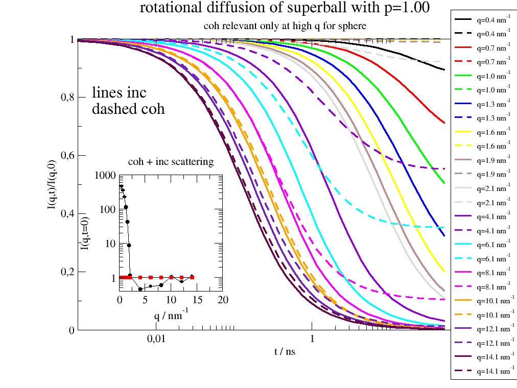
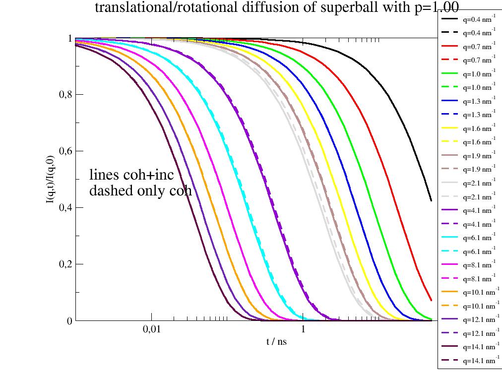
jscatter.dynamic.u2Debye(T, thetaD, amass=1)[source]

u2 based on Debye density of states.

Parameters:

Tfloat: Temperature in K.
thetaDfloat: Debye temperature in K.
amassfloat: Mass of contributing atom in atomic mass units.

Returns:

msd(T)dataArray

Notes

In harmonic approximation the msd has the form

\[<u^2> = \frac{3\hbar}{2m} \int_0^{\omega_m} \frac{1}{\omega} cth(\hbar\omega/2kT)g(\omega) d\omega\]

with m as atomic mass,:mat:hbar as reduced Planck constant, k as Boltzmann constant and $\omega$ as phonon frequencies.

The Debye model assumes $g_D(\omega)=3\omega^2/\omega_D^3$ with the maximum frequency $\omega_D$ related by tothe debye temperatur $\Theta_D=\omega\hbar/k$.

Combination yields

\[msd = <u^2> = \frac{9\hbar^2}{\Theta_D mk} (\frac{1}{4}+\frac{\phi(x_D)}{x_D^2})\]

\[\phi(x_D) = \int_0^{x_D} \frac{x}{e^x-1}dx\]

References

[1]

Bée, M. Quasielastic Neutron Scattering; Adam Hilger, 1988.

jscatter.dynamic.zilmanGranekBicontinious(t, q, xi, kappa, eta, mt=1, amp=1, eps=1, nGauss=60)[source]

Dynamics of bicontinuous micro emulsion phases. Zilman-Granek model as equ B10 in [1]. Coherent scattering.

On very local scales (however larger than the molecular size) Zilman and Granek represent the amphiphile layer in the bicontinuous network as consisting of an ensemble of independent patches at random orientation of size equal to the correlation length xi. Uses Gauss integration and multiprocessing.

Parameters:

tarray: Time values in ns
qfloat: Scattering vector in 1/A
xifloat: Correlation length related to the size of patches which are locally planar and determine the width of the peak in static data. unit A A result of the teubnerStrey model to e.g. SANS data. Determines kmin=eps*pi/xi .
kappafloat: Apparent single membrane bending modulus, unit kT
etafloat: Solvent viscosity, unit kT*A^3/ns=100/(1.38065*T)*eta[unit Pa*s] Water about 0.001 Pa*s = 0.000243 kT*A^3/ns
ampfloat, default = 1: Amplitude scaling factor
epsfloat, default=1: Scaling factor in range [1..1.3] for kmin=eps*pi/xi and rmax=xi/eps. See [1].
mtfloat, default 0.1: Membrane thickness in unit A as approximated from molecular size of material. Determines kmax=pi/mt. About 12 Angstrom for tenside C10E4.
nGaussint, default 60: Number of points in Gauss integration

Returns:

dataList

Notes

See equ B10 in [1] :

\[S(q,t) = \frac{2\pi\xi^2}{a^4} \int_0^1 d\mu \int_0^{r_{max}} dr rJ_0(qr\sqrt{1-\mu^2}) e^{-kT/(2\pi\kappa)q^2\mu^2 \int_{k_{min}}^{k_{max}} dk[1-J_0(kr)e^{w(k)t}]/k^3}\]

with $\mu = cos(\sphericalangle(q,surface normal))$ , $J_0$ as Bessel function of order 0

For technical reasons, in order to avoid numerical difficulties, the real space upper (rmax integration) cutoff was realized by multiplying the integrand with a Gaussian having a width of eps*xi and integrating over [0,3*eps*xi].

References

[1] (1,2,3)

Dynamics of bicontinuous microemulsion phases with and without amphiphilic block-copolymers M. Mihailescu, M. Monkenbusch et al J. Chem. Phys. 115, 9563 (2001); http://dx.doi.org/10.1063/1.1413509

Examples

import jscatter as js
import numpy as np
t=js.loglist(0.1,30,20)
p=js.grace()
iqt=js.dynamic.zilmanGranekBicontinious(t=t,q=np.r_[0.03:0.2:0.04],xi=110,kappa=1.,eta=0.24e-3,nGauss=60)
p.plot(iqt)

# to use the multiprocessing in a fit of data use memoize
data=iqt                          # this represent your measured data
tt=list(set(data.X.flatten))      # a list of all time values
tt.sort()

# use correct values from data for q     -> interpolation is exact for q and tt
zGBmem=js.formel.memoize(q=data.q,t=tt)(js.dynamic.zilmanGranekBicontinious)
def mfitfunc(t, q, xi, kappa, eta, amp):
   # this will calculate in each fit step for for Q (but calc all) and then take from memoized values
   res= zGBmem(t=t, q=q, xi=xi, kappa=kappa, eta=eta, amp=amp)
   return res.interpolate(q=q,X=t)[0]
# use mfitfunc for fitting with multiprocessing

jscatter.dynamic.zilmanGranekLamellar(t, q, df, kappa, eta, mu=0.001, eps=1, amp=1, mt=0.1, nGauss=40)[source]

Dynamics of lamellar microemulsion phases. Zilman-Granek model as Equ 16 in [1]. Coherent scattering.

Oriented lamellar phases at the length scale of the inter membrane distance and beyond are performed using small-angle neutrons scattering and neutron spin-echo spectroscopy.

Parameters:

tarray

Time in ns

qfloat

Scattering vector

dffloat

film-film distance. unit A
This represents half the periodicity of the structure, generally denoted by d=0.5df which determines the peak position and determines kmin=eps*pi/df

kappafloat

Apparent single membrane bending modulus, unit kT

mufloat, default 0.001

Angle between q and surface normal in unit rad. For lamellar oriented system this is close to zero in NSE.

etafloat

Solvent viscosity, unit kT*A^3/ns = 100/(1.38065*T)*eta[unit Pa*s] Water about 0.001 Pa*s = 0.000243 kT*A^3/ns

epsfloat, default=1

Scaling factor in range [1..1.3] for kmin=eps*pi/xi and rmax=xi/eps

ampfloat, default 1

Amplitude scaling factor

mtfloat, default 0.1

Membrane thickness in unit A as approximated from molecular size of material. Determines kmax=pi/mt About 12 Angstrom for tenside C10E4.

nGaussint, default 40

Number of points in Gauss integration

Returns:

dataList

Notes

See equ 16 in [1] :

\[S(q,t) \propto \int_0^{r_{max}} dr r J_0(q_{\perp}r) exp \Big( -\frac{kT}{2\pi\kappa} q^2\mu^2 \int_{k_{min}}^{k_{max}} \frac{dk}{k^3} [1-J_0(kr) e^{w^\infty(k)t}] \Big)\]

with $w^{\infty(k) = k^3\kappa/4\overline{\eta}}$, $\mu = cos(\sphericalangle(q,surface normal))$ ,: $J_0$ as Bessel function of order 0. For details see [1].

The integrations are done by nGauss point Gauss quadrature, except for the kmax-kmin integration which is done by adaptive Gauss integration with rtol=0.1/nGauss k< kmax/8 and rtol=1./nGauss k> kmax/8.

References

[1] (1,2,3)

Neutron scattering study on the structure and dynamics of oriented lamellar phase microemulsions M. Mihailescu, M. Monkenbusch, J. Allgaier, H. Frielinghaus, D. Richter, B. Jakobs, and T. Sottmann Phys. Rev. E 66, 041504 (2002)

Examples

import jscatter as js
import numpy as np
t=js.loglist(0.1,30,20)
ql=np.r_[0.08:0.261:0.03]
p=js.grace()
iqt=js.dynamic.zilmanGranekLamellar(t=t,q=ql,df=100,kappa=1,eta=2*0.24e-3)
p.plot(iqt)
p.yaxis(label=r'I(Q,t)',min=1e-6,max=1)
p.xaxis(label=r'Q / nm\S-1')
# p.save(js.examples.imagepath+'/zilmanGranekLamellar.jpg', size=(2,2))

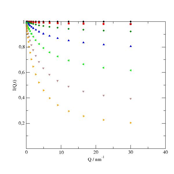
jscatter.dynamic.fft.k = 0.08617333262145178: Boltzmann constant in meV/K

jscatter.dynamic.fft.h = 4.135667696923859: Planck constant in µeV*ns = meV*ps

jscatter.dynamic.fft.hbar = 0.6582119569509066: h/2π reduced Planck constant in µeV*ns = meV*ps