1. Beginners Guide / Help
Analysis of data consists of several steps that can be done with Jscatter :
Reading of measured data
Define a model
Fit your model (test if it describes data)
Save results !!!
These are described in the following.
Some places to start with Python/Numpy/SciPy :
Python-Numpy-Tutorial A crash course with contents as :
Basic data types, Containers (Lists, Dictionaries, Sets, Tuples), Functions, Classes
Numpy, Arrays, indexing, Datatypes, Array math, Broadcasting
How to use, get help and command expansion
Jscatter works in a terminal/shell (open it) as basis without a graphical user interface (GUI).
For convenience we use Ipython (colors highlighting, history, …), start it typing “ipython” in a terminal.
Optionally Jscatter can also be run in an environment like Jupyter-lab (see Jupyter Notebook).
Give it a try using a live demo in a Jupyter Notebook at ![]() to test Jscatter.
to test Jscatter.
In a shell some simple things help the user.
The Python docstring of a function can be retrieved by help(command)
The ‘TAB’ can be used to expand a command or get the list of possible methods/attributes
Just typing the name of an object returns a short representation e.g. the content of a dataArray.
js.showDoc() opens the documentation in a web browser.
import jscatter as js
i5 = js.dL(js.examples.datapath + '/iqt_1hho.dat')

# try with some data from below
help(i5.fit)

# command completion by *TAB*
i5.a    # write this and press 2x *TAB* to get *append, aslist, attr*

# show string representation
i5

js.showDoc()
1.1. What are dataArray/dataList
dataArray is a container for matrix like data like a spreadsheet.
Additional to the entries in the spreadsheet we have attributes describing metadata
(like wavevector, temperature related to the dataArray accessible as data.wavevector.
Additional attributes data.X, data.Y or data.eY allow easy access to X,Y or error Y columns.
This tells plot and fit commands which data to use.
See setColumnIndex() how to change respective columns and more.
Consequently, if calculating something, we use these attributes e.g. to caluclate new Y values as
data.Y = data.Y * (1+data.X)**2 or combining with other dataArrays of same length.
dataList is a container for a list of dataArrays with variable size e.g. for repeated measurements as a temperature scan or a set of measurements for simultaneous fitting.
In most cases experimental data are read from a file, as it was stored from a measurement/instrument. On the other hand model results are in a dataArray/dataList together with attributes used for calulation.
See dataArray and dataList how to create and use both. In short:
import jscatter as js
import numpy as np

x=np.r_[0.1:10:0.5]                                    # creates a 1dim numpy array
array = np.c_[x, x**2, 0.5*np.random.randn(len(x))].T  # creates an array with columns as first index
data = js.dA(array)                                    # creates dataArray from above array

data.temperature = 273.15                              # adds attribute temperature
data.Y = np.log(data.Y) / data.X * data.temperature    # manipulate content

data1 = js.dL()                                        # empty dataList
for i in [1,2,3,4,5]:                                  # add several dataArrays
   # internal a dataArray is created as above and appended to dataList
   data1.append(np.c_[x, x**2+i, 1.234*np.sin(i*3.141*x)].T)
dataArray/dataList have additional methods to treat the contained data. This might be simple mathematical operations like add a value to a column or summing, averaging, adding another array of data as inherited from numpy arrays or methods for fitting and interpolation.
1.2. First basic examples
This shows the basic reading and fitting of some data as a starting point.
Details of all commands are explained later or in respective chapters.
Open an Ipython shell or Jupyter notebook and paste line by line (or block if indented).
A code block has a symbol for copy in the upper right corner to copy.
In Ipython use the magic word paste to paste the previous copied block.
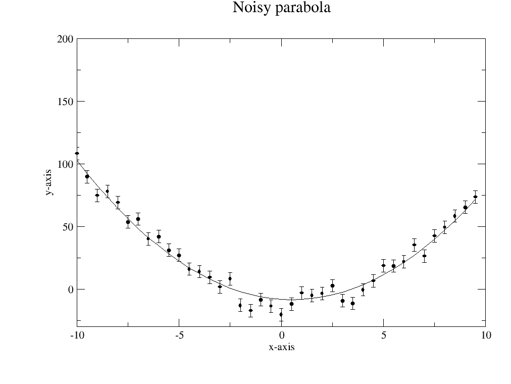
1.2.1. A parabolic fit
A simple 1D example without additional stuff as a skeleton. Additional possibilities are shown later.
Multidimensional examples may use an attribute as second dimension (see Fitting 1D, 2D 3D …)
import jscatter as js
import numpy as np
# load data into a dataArray
data=js.dA(js.examples.datapath+'/exampledata0.dat')
# Look at the data to get an overview
p=js.grace(1,1)
p.plot(data)
# Look at some attributes that were stored in the read data
data.attr # shows a list of attributes as below
data.temperature # contains the temperature found in the file
data.comment # contains a comment
# define model like a mathematical function y = f(q,a,b,c)
# test this using e.g parabola(data.X,1,2,3)
def parabola(q,a,b,c):
# q values as numpy array (a list of values), the model returns an array (the y values)
y = (q-a)**2+b*q+c
return y
# fit the data defining free parameters, fixed parameters and map model names to data names.
# (map data 'X' values (array) to model 'q' parameter.)
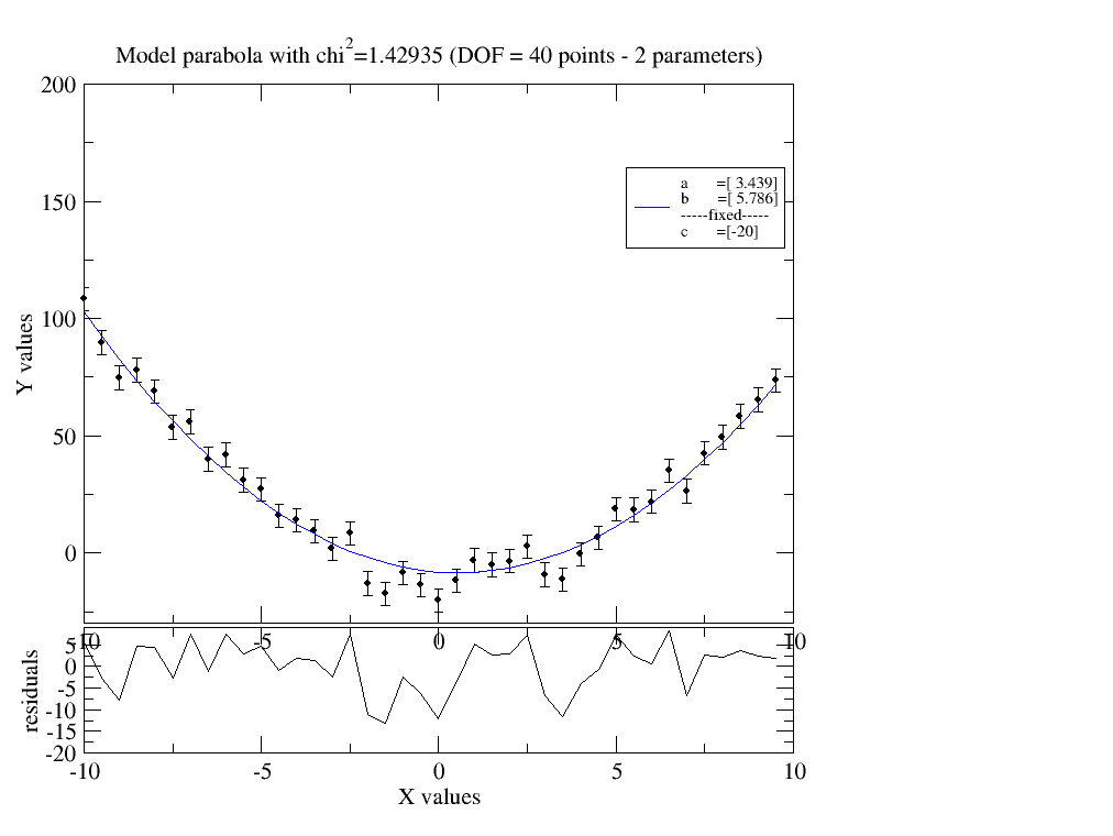
data.fit( model=parabola ,freepar={'a':2,'b':4}, fixpar={'c':-20}, mapNames={'q':'X'})
data.showlastErrPlot()
# map additionally the 'temperature' in the data for parameter 'c'.
# using parameter 'temperature' instead of 'c' in the model will do an automatic mapping.
data.fit( model=parabola ,freepar={'a':2,'b':4}, fixpar={}, mapNames={'q':'X','c':'temperature'})
# make nice plot with data and fit
p=js.grace(1,1)
p.plot(data)
p.plot(data.lastfit,line=1,symbol=0) # add result in lastfit
p.title('Noisy parabola')
# save errplot with residuals and parameters
data.savelastErrPlot('errplot.agr')
1.2.2. A bit more complex data
Here we introduce more possibilities and concepts how to treat the data and introduce models.
Use a model from the libraries or change it to your needs.
Fit with a condition
Simulate fit result with changed parameters.
Use a vectorized quadrature to include the distribution of a parameter.
Access the fit result
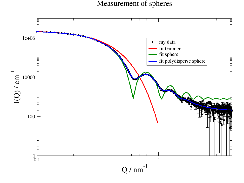
The used data relate to small angle scattering of spherical particles in solvent with a polydispersity in radius.
import jscatter as js
import numpy as np

# load data
data=js.dA(js.examples.datapath+'/exampledata.dat')

# plot data
p=js.grace(1,1)
p.plot(data,le='my data')
p.yaxis(scale='l',label='I(Q) / cm\S-1',size=1.5)
p.xaxis(min=0.1,max=4,scale='l',label='Q / nm\S-1',size=1.5)
p.title('Measurement of spheres')

# use Guinier model from module formfactor (shortcut ff) as first size estimate in limited range q<1/Rg
# fit it (with start values) and show result
data.fit(js.ff.guinier,freepar={'Rg':5,'A':1e6},
                       fixpar={},
                       mapNames={'q':'X'},
                       condition=lambda a:a.X<1/7)

# show fit result (The ErrPlot is reused in next fits)
data.showlastErrPlot(yscale='log',fitlinecolor=5)

# compare to full dataset in above plot
# modelValues recalcs fit result with optional changed parameters (here larger q range)
p.plot( data.modelValues(q=np.r_[0.1:1:0.02]), line=[1,3,2], symbol=0, legend='fit Guinier')
p.legend(x=0.8,y=1e6)          # update legend with position

# define monodisperse sphere model adding amplitude and background
# jscatter models return dataArray with X, Y and more attributes
# you may return just an array
def sphere(q,R,A,bgr):
   result=A*js.ff.sphere(q=q,radius=R).Y+bgr
   return result

# use sphere model (keywords as *freepar* can be dropped if order of keywords is preserved)
data.fit(sphere,{'R':5,'A':1,'bgr':50},{},{'q':'X'})

p.plot(data.modelValues(q=data.X), li=[1,3,3], sy=0, le='fit sphere')
p.legend()

# define better sphere model with polydisperse radius
# here we reuse the returned dataArray (which includes attributes) and add bgr attribute.
def psphere(q,R,A,bgr,dR):
   # dR is radius width of a Gaussian centered at R (see doc of pDA)
   result=js.formel.pDA(js.ff.sphere,dR,'radius',q=q,radius=R)
   result.Y = A * result.Y + bgr
   result.bgr = bgr
   return result

# use the polydisperse sphere model
data.fit(psphere,{'R':5,'A':1,'bgr':50,'dR':1},{},{'q':'X'})

p.plot(data.modelValues(q=np.r_[0.1:4:0.04]), li=[1,3,4], sy=0, le='fit polydisperse sphere')
p.legend(x=0.8,y=1e6)
p.xaxis(min=0.1,max=4)
# p.save('myevaluation.agr')
# p.save('myevaluation.png')

# look at result with parameters with errors
data.lastfit          # model data
data.lastfit.R        # fit parameter
data.lastfit.R_err    # fit parameter 1-sigma error
data.lastfit.dR
data.lastfit.dR_err

# save the fit result including the fit parameters, errors and covariance matrix
data.lastfit.save('myevaluationfitresult.dat')
1.3. Reading ASCII files
A common problem is how to read ASCII files with data. The data format is often not very intuitive designed. Often there is additional metadata before or after a matrix like block or in the filename.
Jscatter uses a simple concept to classify/interpret lines :
2 numbers at the beginning of a line are data (matrix like data block).
a name followed by at least one number (and more) is an attribute with name and content (everything after the name).
everything else is comment (but can later be converted to an attribute).
The filename is always stored in attribute
.name
A new dataArray is created if, while reading a file, a data block with an attribute block (preceded or appended) is found or a keyword indicates it (see
dataListparameter block).
Even complex ASCII files can be read with a few changes given as options to fit into this concept (e.g. deleting needless characters like separating ‘:’ or ‘;’ ).
New attributes can be generated from content of the comments if not detected automatically. This can be done during reading using some simple options in dataArray/dataList creation:
dataArray (short: js.dA) reads one dataset from a file.
# create single dataArray from file
dat = js.dA('singledatafilename.dat')            # take dataset in file
dat = js.dA('multidatafilename.dat',index=2)     # take dataset index=3 in file (indices start with 0)
dataList (short: js.dL) reads all datasets from one/multiple files (which may differ in shape)
# create dataList
data = js.dL('../data/latest_0001.dat')          # read all dataset in file
data = js.dL('../data/latest_0001.dat',index=2)  # select only the second dataset in the file
data.append(dat)                                 # append single dataArray read from above
Read all, filter later Create dataList from multiple files (uses glob.glob(pathname,recursive=True) patterns)
data = js.dL('./data/lat*.dat')              # reads all '.dat' files starting with 'lat' in data folder.
data = js.dL('./data/a*/lat*.dat')           # same but reads in subfolders of data folder starting with 'a'
data = js.dL('./data/**/lat*.dat')           # same but recursively reads in all subfolders of data folder

# same with glob (using name patterns as ?, *, **)
import glob
data=js.dL()  # empty dataList
for filename in glob.glob('../data/latest*.dat'):
   data.append(filename)                            # you may add options
   data[-1].Q = float(filename.split('_')[2])       # add attributes from filename (== data[-1].name)
Filter large dataList according to content. The full filename including the path is in
.name# filter according to attributes or name data2 = data.filter(lambda a:a.name.startswith('latest_conc2') & (a.Temp>100)) data3 = data[1:-1:3] # drop first and last and use only each 3rd # add attributes e.g. from filename or comments for dat in data: dat.Temp = float(dat.name.split('_')[2]) # extract attribute from name (which is always the filename read from) dat.pressure = dat.comment[1].split()[1] # if second comment line contains 'pressure 1000 mbar'
Options to change file contents (examples below).
See dataArray() for all options and how to use them. :
replace={‘old’:’new’, ’,’:’.’, 'None':''}==> replace char and strings in text lines before interpretationskiplines=lambda words: any(w in words for w in [‘’,’ ‘,’NAN’,’*’])==> skip complete bad linestakeline='ATOM'==> select specific linesignore='#'==> skip lines starting with this characterusecols=[1,2,5]==> select specific columns e.g. for inhomogenous shaped datalines2parameter=[2,3,4]==> use these data lines as comment and not as data. E.g. for header lines of numbers.
If there is more information in comments or filename this can be extracted by using the comment lines.
data.getfromcomment('nameatfirstcolumn')==> extract a list of words in this linedata.name==> filename, see below examples.
Set columns for X,.Y,.Z,.W and respective errors by
data.setColumnIndex(ix=2,iy=4,iey=None)to pick the columns that are for interest. See Manipulating dataArray/dataList
How to extract information from comment lines and filenames
Lines as pressure 1013 14 are used automatically to set an attribute as .pressure.
Filenames (saved on .name) can be used to save attributes during measurements
(Use speaking filenames during your measurement!)
# data.name is a string as 'adh_Temp273_conc02.dat' extract Temp and conc like
temp=data.name.split('_')  # a list of strings
data.Temp = float(temp[1][4:])
data.conc = float(temp[2][4:6])
#
# if same line is in comment use
temp = data.comment[0].split('_')
# or use data.getfromComment(...)
Some examples and how to read them
filename: data1_10mM.dat (similar to Instrument JNSE (Phoenix), Garching or CHRNS NSE (NIST, Washington)). This data structure was the original design goal.
Sample2 Thu Dec  5 12:55:32 2013
Sampl_10 Sqt/Sq  vs tau/ns     16890000
parameter
q               0.080000
trans_fak       0.877193
volf_bgr        1.000000
temp          273.000000
ref            16790
bgr            16903 1 3
detectorsetting up

0.854979E-01  0.178301E+03  0.383044E+02
0.882382E-01  0.156139E+03  0.135279E+02
0.909785E-01  0.150313E+03  0.110681E+02
0.937188E-01  0.147430E+03  0.954762E+01
0.964591E-01  0.141615E+03  0.846613E+01
....
Read by
data=js.dA('data1_273K_10mM.dat')
# optional ::
data.getfromComment('detectorsetting')           # creates attribute detectorsetting with string value 'up' found in comments
data.conc=float(data.name.split('_')[2][:-2])    # extract from filename
data.q                                           # use Q value  # this was created automatically
data.temp                                        # use temperature value   # th
NSE measurement from IN15 at ILL Grenoble (filename is ‘017112345.txt’). An older version, meanwhile Amplitude and Polarisation are in a different file.
ftime          E_SUM           EERR_SUM        EQ_0.0596       EERRQ_0.0596    EQ_0.0662       EERRQ_0.0662    EQ_0.0728       EERRQ_0.0728    EQ_0.0793       EERRQ_0.0793    EQ_0.0859       EERRQ_0.0859
Amplitude       -1.0000e+00      0.0000e+00      3.3149e+00      1.9984e-03      3.4203e+00      2.0375e-03      3.2560e+00      1.9803e-03      2.7188e+00      1.8161e-03      1.8634e+00      1.5032e-03
Polarisation    -1.0000e+00      0.0000e+00      2.3719e+00      4.4403e-03      2.3723e+00      4.6673e-03      2.1675e+00      4.6726e-03      1.7156e+00      4.4392e-03      1.1127e+00      3.7890e-03
 0.0000e+00      1.0000e+00      1.0318e-03      1.0000e+00      1.9261e-03      1.0000e+00      2.0252e-03      1.0000e+00      2.2186e-03      1.0000e+00      2.6615e-03      1.0000e+00      3.4992e-03
 2.2428e-01      9.7447e-01      3.4201e-03      9.7363e-01      6.3708e-03      9.7026e-01      6.6990e-03      9.8392e-01      7.3605e-03      9.8819e-01      8.8623e-03      9.5632e-01      1.1831e-02
 2.9474e-01      9.8425e-01      3.3694e-03      9.9020e-01      6.1962e-03      9.7785e-01      6.5809e-03      9.9125e-01      7.2723e-03      9.8005e-01      8.8698e-03      9.9022e-01      1.1909e-02
 3.6520e-01      9.7910e-01      3.3071e-03      9.8269e-01      6.0875e-03      9.8190e-01      6.4363e-03      9.7275e-01      7.1155e-03      9.8566e-01      8.7117e-03      9.7766e-01      1.1829e-02
 5.0612e-01      9.7927e-01      3.2226e-03      9.7898e-01      5.9112e-03      9.7517e-01      6.2379e-03      9.8108e-01      6.9563e-03      9.8669e-01      8.5569e-03      9.8611e-01      1.1557e-02
 ...
Read by
# column 1,2 are averages over following columns. First line contains q values
data=js.dL()   # empty dataList
temp=js.dA('017112345.txt')         # read all then sort later
for i in [3,5,7,9]:
   data.append(temp[[0,i,i+1]])
   data[-1].Amplitude=temp.Amplitude[i-1:i+1]
   data[-1].Polarisation=temp.Polarisation[i-1:i+1]
   data[-1].q=float(temp.comment[0].split()[i].split('_')[1])
.inx files used at backscattering and TOF instruments
Not everything is given in these files and its difficult to find documentation and different versions exist. Ask you local contact how it was used.
First line: number_of_channels - - - - - number_of_lines
Second line: angle_or_Q incident_energy Q - - -
Position in line is important (prepared to have >1000 chanels) so spaces count for block.
typically such a block for each detector without separation.
A first space is missing below. Inspect the file in the example.
This is from SPHERES@MLZ :
562    1   2   0   0   0   0 559
  title...
   0.1659    2.0802    0.0000    0.0000    0.0000    0.0000
 0.0000000       0.000000       0.000000
   1 -22.24000 1.85168e+00 7.18052e-02
   2 -22.16000 1.90019e+00 1.11010e-01
   3 -22.08000 1.70560e+00 1.20304e-01
   .....
 558  22.32000 1.72710e+00 1.00386e-01
 559  22.40000 1.62634e+00 8.61959e-02
Another version of the format of .inx files used at backscattering and TOF instruments at ILL. Now we have different spaces obviously different meanings but roughly the same structure.
  943    1    2    0    0    0    0  940
Local segmental dynamics in polymer
 2.4600   2.272  1.0472  353.030   1.0 0
                  0.0000  9.7656  0.0000
     -49.37293  0.00000e+00 -1.0000e+00
     -48.58932  0.00000e+00 -1.0000e+00
     -47.82341  0.00000e+00 -1.0000e+00
     -47.07465  0.00000e+00 -1.0000e+00
  943    1    2    0    0    0    0  940
Local segmental dynamics in polymer
 2.4800   2.272  1.0472  353.030   1.0 0
                  0.0000  9.7656  0.0000
      -49.37293  0.00000e+00 -1.0000e+00
      -48.58932  0.00000e+00 -1.0000e+00
      -47.82341  0.00000e+00 -1.0000e+00
      -47.07465  0.00000e+00 -1.0000e+00
      -46.34256  0.00000e+00 -1.0000e+00
Read using this function to extract additional parameters using lines2parameter
import jscatter as js
import numpy as np

def readinx(filename, block=' 562 '):
    # reusable function for inx reading
    # neutron scatterers use strange data formats like .inx
    # the blocks start with  number of channels.
    # Spaces are important (' 562 ') to find the starting line.
    # this might dependent on instrument and somtimes there are additional lines in same experiment
    data = js.dL(filename,
                 block=block,                    # this finds the starting of the blocks of all angles or Q
                 usecols=[1,2,3],                # ignore the numbering at each line
                 lines2parameter=[-1,-2,-3,-4])  # catch the parameters at beginning
    for da in data:
        da.channels = da.line_1[0]
        da.Q = da.line_3[0]                       # angle but sometimes also Q
        da.incident_energy = da.line_3[1]         # in meV
        da.QQ = da.line_3[2]                       # here should be Q
        da.temperature = da.line_3[3]              # in K if given
    return data

    # read data
    vana = readinx(js.examples.datapath +'/Vana.inx.gz',block=' 562 ')
aspirin.pdb: Atomic coordinates for aspirin (AIN from Protein Data Bank, PDB ):
Header
Remarks blabla
Remarks in pdb files are sometimes more than 100 lines
ATOM      1  O1  AIN A   1       1.731   0.062  -2.912  1.00 10.00           O
ATOM      2  C7  AIN A   1       1.411   0.021  -1.604  1.00 10.00           C
ATOM      3  O2  AIN A   1       2.289   0.006  -0.764  1.00 10.00           O
ATOM      4  C3  AIN A   1      -0.003  -0.006  -1.191  1.00 10.00           C
ATOM      5  C4  AIN A   1      -1.016   0.010  -2.153  1.00 10.00           C
ATOM      6  C5  AIN A   1      -2.337  -0.015  -1.761  1.00 10.00           C
ATOM      7  C6  AIN A   1      -2.666  -0.063  -0.416  1.00 10.00           C
ATOM      8  C1  AIN A   1      -1.675  -0.085   0.544  1.00 10.00           C
ATOM      9  C2  AIN A   1      -0.340  -0.060   0.168  1.00 10.00           C
ATOM     10  O3  AIN A   1       0.634  -0.083   1.111  1.00 10.00           O
ATOM     11  C8  AIN A   1       0.314   0.035   2.410  1.00 10.00           C
ATOM     12  O4  AIN A   1      -0.824   0.277   2.732  1.00 10.00           O
ATOM     13  C9  AIN A   1       1.376  -0.134   3.466  1.00 10.00           C
ATOM     14  HO1 AIN A   1       2.659   0.080  -3.183  1.00 10.00           H
ATOM     15  H4  AIN A   1      -0.765   0.047  -3.203  1.00 10.00           H
ATOM     16  H5  AIN A   1      -3.119   0.001  -2.505  1.00 10.00           H
ATOM     17  H6  AIN A   1      -3.704  -0.082  -0.117  1.00 10.00           H
ATOM     18  H1  AIN A   1      -1.939  -0.123   1.591  1.00 10.00           H
ATOM     19  H91 AIN A   1       0.931  -0.004   4.453  1.00 10.00           H
ATOM     20  H92 AIN A   1       1.807  -1.133   3.391  1.00 10.00           H
ATOM     21  H93 AIN A   1       2.158   0.610   3.318  1.00 10.00           H
CONECT    1    2   14 may appear at the end
HETATOM lines may appear at the end
END
Read by (several methods):
# 1.
# take 'ATOM' lines, but only column 6-8 as x,y,z coordinates.
js.dA(js.examples.datapath+'/AIN_ideal.pdb',takeline='ATOM',replace={'ATOM':'0'},usecols=[6,7,8])
# 2.
# replace 'ATOM' string by number and set XYZ for convenience
js.dA(js.examples.datapath+'/AIN_ideal.pdb',replace={'ATOM':'0'},usecols=[6,7,8],XYeYeX=[0,1,None,None,2])
# 3.
# only the Oxygen atoms
js.dA(js.examples.datapath+'/AIN_ideal.pdb',takeline=lambda w:(w[0]=='ATOM') & (w[2][0]=='O'),replace={'ATOM':'0'},usecols=[6,7,8])
# 4.
# using regular expressions we can decode the atom specifier into a scattering length
import re
rHO=re.compile('HO\d') # 14 is HO1
rH=re.compile('H\d+')  # represents something like 'H11' or 'H1' see regular expressions
rC=re.compile('C\d+')
rO=re.compile('O\d+')
# replace atom specifier by number and use it as last column
ain=js.dA(js.examples.datapath+'/AIN_ideal.pdb',replace={'ATOM':'0',rC:1,rH:5,rO:2,rHO:5},usecols=[6,7,8,2],XYeYeX=[0,1,None,None,2])
# 5.
# read only atoms and use it to retrieve atom data from js.formel.Elements
atoms=js.dA('AIN_ideal.pdb',replace={'ATOM':'0'},usecols=[2],XYeYeX=[0,1,None,None,2])[0].array
al=[js.formel.Elements[a[0].lower()] for a in atoms]
A file with a lot of errors.
data2.txt:
# this is just a comment or description of the data
# temp     ;    293
# pressure ; 1013 14  bar
# name     ; temp1bsa
&doit
0,854979E-01  0,178301E+03  0,383044E+02
0,882382E-01  0,156139E+03  0,135279E+02
0,909785E-01  *             0,110681E+02
0,937188E-01  0,147430E+03  0,954762E+01
0,964591E-01  0,141615E+03  0,846613E+01
nan           nan           0
Read by
# ignore is by default '#', so switch it of
# skip lines with non numbers in data
# replace some char by others or remove by replacing with empty string ''.
js.dA('data2.txt',replace={'#':'',';':'',',':'.'},skiplines=[‘*’,'nan'],ignore='' )
pdh format used in some SAXS instruments (first real data point is line 4):
SAXS BOX
      2057         0         0         0         0         0         0         0
  0.000000E+00   3.053389E+02   0.000000E+00   1.000000E+00   1.541800E-01
  0.000000E+00   1.332462E+00   0.000000E+00   0.000000E+00   0.000000E+00
-1.069281E-01   2.277691E+03   1.168599E+00
-1.037351E-01   2.239132E+03   1.275602E+00
-1.005422E-01   2.239534E+03   1.068182E+00
-9.734922E-02   2.219594E+03   1.102175E+00
......
Read by:
# this saves the prepended lines in attribute line_2,...
empty=js.dA('exampleData/buffer_averaged_corrected_despiked.pdh',usecols=[0,1],lines2parameter=[2,3,4])
# next just ignores the first lines (and last 50) and uses every second line,
empty=js.dA('exampleData/buffer_averaged_corrected_despiked.pdh',usecols=[0,1],block=[5,-50,2])
Read csv data by (comma separated list)
js.dA('data2.txt',replace={',':' '})
# If tabs separate the columns
js.dA('data2.txt',replace={',':' ','\t':' '})
Get a list of files in a folder or recursive in all subfolders with path + names
import glob
# current folder
files = glob.glob('latest*.dat')     # files starting with 'latest' and ending '.dat' in current folder
files = glob.glob('lat???.dat')   # files starting with 'lat' and ending '.dat' and 3 char in between; current folder

# subfolders
files = glob.glob('dir1/*.dat')   # '.dat' files in 'dir1' folder
files = glob.glob('dir*/*.dat')   # '.dat' files in all folders starting with 'dir'

# recursive subfolders, filter after reading according to names and attributes
files = glob.glob('di/**/*.dat',recursive=True)  # '.dat' files in all recursive subfolders of 'di'

# filter it before reading to select a subset
ifwsfiles = list(filter(lambda a:'IFWS' in a,files))

# read all the files
alldata = js.dL(files)
IFWSdata = js.dL(ifwsfiles)
If you get errors it might be that single files have a strange format that the dL options need to be adapted.
1.4. Creating from numpy arrays
This demonstrates how to create dataArrays with calculated data and corresponding errors:
x=np.r_[0:10:0.5]                 # a list of values
D,A,q=0.45,0.99,1.2               # parameters
data=js.dA(np.vstack([x,  np.exp(-q**2*D*x)+np.random.rand(len(x))*0.05,  x*0+0.05]))
data.diffusioncoefficient=D
data.amplitude=A
data.wavevector=q

# alternative (diffusion with noise and error )
data=js.dA(np.c_[x,np.exp(-q**2*D*x)*0.05,x*0+0.05].T)
# or
def diffusion(t,D0,Q,e):
   return np.exp(-Q**2*D0*t)+np.random.rand(len(t))*e
data=js.dA(np.c_[x,diffusion(t=x,D0=D,Q=q,e=0.05),np.zeros_like(x)+0.05].T)

# save data
data.save('my_simulated_data.dat')
# read later
data = js.dA('my_simulated_data.dat')
1.5. Manipulating dataArray/dataList
Changing values uses the same syntax as in numpy arrays with all available methods and additional .X,.Y…
The columns used for .X,.Y,.Z,.W and respective errors can be changed by .setColumnIndex(ix=2,iy=4,iey=None) . Later .Y is used during fits as dependent variable.
Default ix,iy,iey = 0,1,2 as one expects this
When writing data the attribute line
XYeYeX 0 1 2 - - - - -is used to save the column indices in sequence as given inprotectedNames()-> X, Y, eY, eX, Z, eZ, W, eW. When reading the file this attribut information is used to recover the column indices. If the line is missing the default0 1 2is used.
dataList elements should be changed individually as dataArray (this can be done in loops)
i7=js.dL(js.examples.datapath+'/polymer.dat')
for ii in i7:
   ii.X/ = 10                 # change scale
   ii.Y/ = ii.conc            # normalising by concentration
   ii.Y = -np.log(ii.Y)*2     # take log

# attributes can be accessed from dataList as list or array
i7.Temp
Tmean = i7.Temp.array.mean()

i1=js.dA(js.examples.datapath+'/a0_336.dat')
# all the same to multiply .X by 2
i1.X *= 2
i1[0] *= 2
i1[0] = i1[0]*2        # most clear writing

# multiply each second Y value by 2 (using advanced numpy indexing)
i1[1,::2]=i1[1,::2]*2
# now more strange: each second gets the value from following *2+1
# unlimited possibilities to manipulate data :-)
i1[1,::2]=i1[1,1::2]*2+1 + i1[2,1::2]

# making a Kratky plot
p=js.grace()
i1k=i1.copy()
i1k.Y=i1k.Y*i1k.X**2
p.plot(i1k)
# or
p.plot(i1.X*10,i1.Y*i1.X**2)
1.6. Indexing dataArray/dataList and reducing
Basic Slicing and Indexing/Advanced Indexing/Slicing works as described at numpy indexing .
This means accessing parts of the dataArray/dataList by indexing with integers, boolean masks or arrays to extract/manipulate a subset of the data.
[A,B,C] in the following describes A dataList, B dataArray columns and C values in columns.
The start:end:step notation is used. With missing value start equals 0, end the last and step 1.
i5=js.dL(js.examples.datapath+'/iqt_1hho.dat')
# remove first 2 and last 2 datapoints in all dataArrays
i6=i5[:,:,:2:-2]
# remove first column and use 1,2,3 columns in all dataArrays
i6=i5[:,1:4,:]
# use each second element in dataList and remove last 2 datapoints in all dataArrays
i6=i5[::2,:,:-2]
# You can loop over the dataArrays
for dat in i5:
   dat.X=dat.X*10
# select a subset by explicit list
i7=i5[[2,3,5,6,]]
Reducing data to a lower number of values can be done by above fancy indexing (loosing data)
or using data.prune (see dataList )
prune reduces e.g by 2000 points by averaging in intervals to get 100 points.
i7=js.dL(js.examples.datapath+'/a0_336.dat')
# mean values in interval [0.1,4] with 100 points distributed on logscale
i7_2=i7.prune(lower=0.1,upper=4,number=100,kind='log') #type='mean' is default
dataList can be filtered to use a subset e.g. with restricted attribute values as .q>1 or temp>300 .
i5=js.dL(js.examples.datapath+'/iqt_1hho.dat')
i6=i5.filter(lambda a:a.q<2)
i6=i5.filter(lambda a:a.q in [1,2,3,4,5])
i6=i5.filter(temp=300)         # automatically sorted for these attributes
This demonstrates how to filter data values according to some rule.
x=np.r_[0:10:0.5]
D,A,q=0.45,0.99,1.2               # parameters
rand=np.random.randn(len(x))      # the noise on the signal
data=js.dA(np.vstack([x,np.exp(-q**2*D*x)+rand*0.05,x*0+0.05,rand])) # generate data with noise
# select like this
newdata=data[:,data[3]>0]         # take only positive noise in column 3
newdata=data[:,data.X>2]          # X>2
newdata=data[:,data.Y<0.9]        # Y<0.9
1.7. Fitting experimental data
We need:
Data need to be read and prepared.
Data may be a single dataset (usually in a dataArray) or several of these (in a dataList) like multiple measurements with same or changing parameters (e.g. wavevectors). Coordinates are in .X and values in .Y See 1D fits with attributes and 2D fit with attributes
2D data (e.g. a detector image with 2 dimensions) need to be transformed to coordinates .X, .Z with values in .Y. This also gives pixels coordinates in an image a physical interpretation as e.g. wavevectors. See examples 2D fitting using .X, .Z, .W and Fitting the 2D scattering of a lattice
Attributes need to be extracted from read data (from comments or filename or from a list). In the below example the temperature is stored in the data as attribute.
A model, which can be defined in different ways. See below or in How to build simple models for different ways.
Lists as parameters are NOT allowed as list are used to discriminate between common parameters (a single float) and individual fit parameters (a list of float for each) in dataList.
Fit algorithm We use mainly methods from scipy.optimize that are incorporated in the .fit method of dataArray/dataList. Additional emcee for Baysian fits is used. The intention is to have the same interface for different fit methods to switch easily still allowing fine tuning if needed.
Most important .fit algorithms are (see
fit()for examples and differences) :
method=’lm’ (default) is what you usually expect by “fitting” including error bars (and a covariance matrix for experts….). It is a wrapper around MINPACK’s lmdif and lmder, which is a modification of the Levenberg-Marquardt algorithm. Errors are 1-sigma errors as they are calculated from the covariance matrix and not directly depend on the errors of the .eY. Still the relative weight of values according to .eY is relevant. Here a numerical approximation for the gradient is used to determine the next step. Methods ‘trf’ and ‘dogbox’ are variants with bounds.
method=’Nelder-Mead’ Nelder-Mead (downhill simplex method) algorithm is a direct search method based on function comparison and sometimes converges when gradient methods fail (or stuck in local minima). However, the Nelder–Mead technique is a heuristic search method that can converge to non-stationary point. It returns no error and is slower than ‘leastsquare’. Nelder-Mead is able to fit data with integer parameters where a gradient method fails.
method=’differential_evolution’ Differential_evolution is a global optimization method using iterative improving candidate solutions. In general it needs a large number of function calls but may find a global minimum.
method=’bayes’ uses Bayesian inference for modeling and the MCMC algorithms for sampling. See emcee for a detailed description of the algorithm. Requires a larger amount of function evaluations but returns errors from Bayesian statistical analysis.
method=’BFGS’ Broyden–Fletcher–Goldfarb–Shanno (BFGS) algorithm. Also a gradient method like ‘lm’. Not as fast as ‘lm’ but gives also error bars.
method=’CG’, ….. and other from scipy.optimize.minimize. These are slower converging than ‘lm’ and most give no error bars. Some require an explicit gradient function ore more. They are more for advanced users if someone really knows why using it in special cases.
Regularized_least_squares use regularisation to constrain the problem by a penalty function e.g. to include prior knowledge about parameters and is connected to Baysian prior . Here above \(\chi^2 minimization\) methods can be used with additional penalty function. For Ridge regression \(\mathbf{\chi_{red}^2} + \lambda \sum_i w_i^2)\) is minimized where for \(\lambda=0\) the conventional \(\chi_{red}^2 minimization\) is retrieved. See Regularisation for fitting for details.
Warning
Save results !!!
Save the fit result !!! I regularly have to ask PhD students “What are the errors ?” and they repeat all their work again. Fit results without errors are often meaningless.
Resulting model Y, parameters with errors are in .lastfit; use data.lastfit.save(‘result.dat’)
errPlot can be saved by data.savelastErrPlot(‘errplot.agr’) or as ‘.jpg’.
If the fit finishes it tells if there was success or if it failed. For error messages the final parameters are no valid fit results!!! Please always check this.
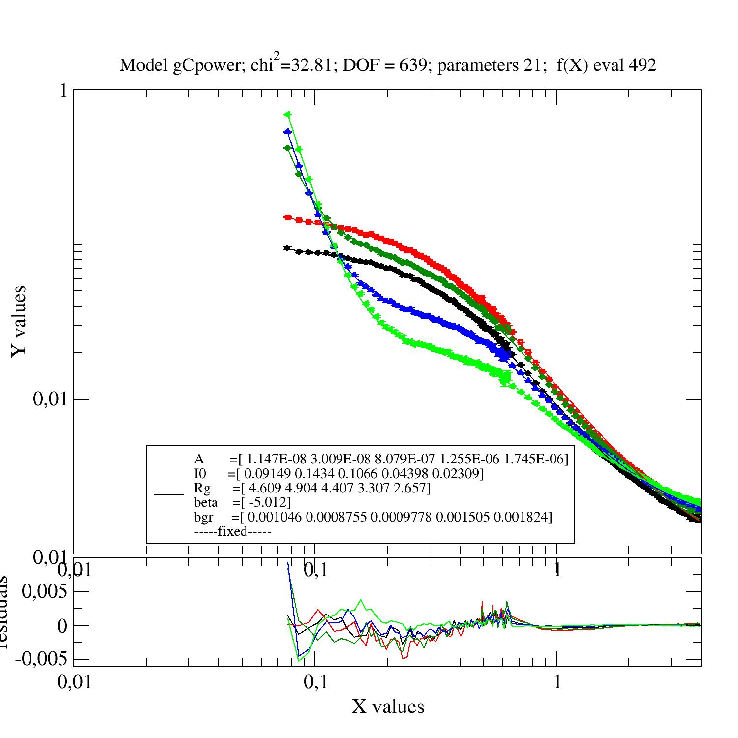
Example A typical example of several datasets from a SAXS measurement.
These are real data of a polymer in solution measured at different temperatures. We observe the collapse of the polymer chain and aggregation.
The first model can still be improved to include the chain stiffness within the wormlikeChain model. In a Kratky plot (YX² vs. X) the characteristic high Q increase is observed. One may limit the Q range to lower Q where the chain stiffness is not visible.
import jscatter as js
import numpy as np
# read data
data=js.dL(js.examples.datapath+'/polymer.dat')
# merge equal Temperatures each measured with two detector distances
data.mergeAttribut('Temp',limit=0.01,isort='X')
# define model
# q will get the X values from your data as numpy ndarray.
def gCpower(q,I0,Rg,A,beta,bgr):
"""Model Gaussian chain + power law and background"""
gc=js.ff.gaussianChain(q=q,Rg=Rg)
# add power law and background
gc.Y=I0*gc.Y+A*q**beta+bgr
# add attributes for later documentation, these are additional content of lastfit (see below)
gc.A=A
gc.I0=I0
gc.bgr=bgr
gc.beta=beta
gc.comment=['gaussianChain with power law and bgr','a second comment']
return gc
data.makeErrPlot(yscale='l',xscale='l') # additional errorplot with intermediate output
data.setlimit(bgr=[0,1]) # upper and lower soft limit
# here we use individual parameter ([]) for all except a common beta ( no [] )
# please try removing the [] and play with it :-)
# mapNames tells that q is *.X* (maps model names to data names )
# condition limits the range to fit (may also contain something like (a.Y>0))
data.fit(model=gCpower,
freepar={'I0':[0.1],'Rg':[3],'A':[1],'bgr':[0.01],'beta':-3},
fixpar={},
mapNames={'q':'X'},
condition =lambda a:(a.X>0.05) & (a.X<4))
# or in short form without condition
data.fit(gCpower,{'I0':[0.1],'Rg':[3],'A':[1],'bgr':[0.01],'beta':-3},{},{'q':'X'})
data.errplot.legend(x=0.02,y=0.005)
# to save errplot
# data.savelastErrPlot(js.examples.imagepath+'/polymerexample.jpg',size=(1.2,1.2)) # to save errplot
# inspect a resulting parameter and error and plot it
data.lastfit.Rg
data.lastfit.Rg_err
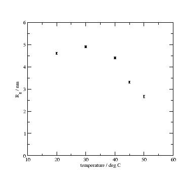
p=js.grace()
p.plot(data.Tempmean,data.lastfit.Rg,data.lastfit.Rg_err,le='radius of gyration')
p.xaxis(label=r'temperature / deg C', min=10, max =60)
p.yaxis(label=r'R\sg\N / nm', min=0, max =6 )
# p.save(js.examples.imagepath+'/polymerexampleRgvsT.jpg',size=(1.2,1.2))
# as result dataArray
result=js.dA(np.c_[data.Tempmean,data.lastfit.Rg,data.lastfit.Rg_err].T)
p.plot(result,le='Rg')
# save the fit result including parameters, errors and covariance matrix
# and your model description
data.lastfit.save('polymer_fitDebye.lastfit.dat')
Errplot with residuals and Rg vs. temperature
In the above example one may fix a parameter. Move it (here ‘bgr’) to the fixpar dict (bgr is automatically extended to correct length).
data.fit(model=gCpower,
         freepar={'I0':[0.1],'Rg':[3],'A':[1]},
         fixpar={'bgr':[0.001, 0.0008, 0.0009],'beta':-4},
         mapNames={'q':'X'},
         condition =lambda a:(a.X>0.05) & (a.X<4))
You may want to fit dataArray in a dataList individually. Do it in a loop.
# from the above
for dat in data:
   dat.fit(model=gCpower,
        freepar={'I0':0.1,'Rg':3,'A':1,},
        fixpar={'bgr':0.001,'beta':-3},
        mapNames={'q':'X'},
        condition =lambda a:(a.X>0.05) & (a.X<4))

# each dataArray has its own .lastfit, .errPlot and so on
data[0].showlastErrPlot()
# for saving with individual names
for dat in data:
   dat.lastfit.save(f'fitresult_Temp{dat.Tempmean:.2f}.dat')
Simulate using the fit result
To simulate how a certain parameter influences the result we may simulate changes in the best fit parameters to observe how model values are changing.
To simulate we may use .modelValues to get an explicit result or use .showlastErrPlot to observe the changes in an errPlot. We just add the new parameter when using these functions. Without parameters we get the original values.
# after a fit we may use it like this
simulated_data = data.modelValues(Rg=4)
# plot it in the errplot with residuals
data.showlastErrPlot(Rg=4,A=2)
1.8. Why Fits may fail
If your fit fails it is most not an error of the fit algorithm even if it sticks somewhere. Read the message at the end of the fit it gives a hint what happened.
If your fit results in a not converging solution or maximum steps reached then its not a valid fit result. Decrease tolerance (‘ftol’, ‘gtol’, ‘tol’), increase ‘max_nfev’ or reduce number of parameter to get a valid result. Try more reasonable start parameters.
Your model may have dependent parameters. Then the gradient cannot be evaluated (and the covariance matrix cannot be calculated). Think of it as a valley with a flat ground. Then you have a line as minimum but you ask for a point. Try a method without gradient.
Your starting parameters are way of and within the first try the algorithm finds no improvement as the steps are quite small. This may happen if you have a dominating function of high power and bad starting parameters. Choose better ones or
diff_step=0.01which increases the first steps.You may run into a local minimum which also depends on the noise in your data. Try :
different start parameters
For ‘lm’ e.g increase step width e.g.
diff_step=0.01(like jumping over the noise/local minima) and with the solution as new start parameters decreasediff_step.Use a more robust method like ‘Nelder-Mead’
or a global optimization method.
Play with the starting parameters and get an idea how parameters influence your function. This helps to get an idea what goes wrong.
And finally :
You have chosen the wrong model ( not correlated to your measurement), units are wrong by orders of magnitude, missing contributions, ….. So read the docs of the models and maybe choose a better one.
1.9. Plot experimental data and fit result
# plot data
p=js.grace()
p.plot(data,legend='measured data')
p.xaxis(min=0.07,max=4,scale='l',label='Q / nm\S-1')
p.yaxis(scale='l',label='I(Q) / a.u.')
# plot the result of the fit
p.plot(data.lastfit,symbol=0,line=[1,1,4],legend='fit Rg=$radiusOfGyration I0=$I0')
p.legend()

p1=js.grace()
# Tempmean because of previous mergeAttribut; otherwise data.Temp
p1.plot(data.Tempmean,data.lastfit.Rg,data.lastfit.Rg_err)
p1.xaxis(label='Temperature / C')
p1.yaxis(label='Rg / nm')
1.10. Save data and fit results
Jscatter saves files in a ASCII format including attributes that can be reread including the attributes (See first example above and dataArray help). In this way no information is lost.
data.save('filename.dat')
# later read them again
data=js.dA('filename.dat')  # retrieves all attributes
If needed, the raw numpy array can be saved (see numpy.savetxt). All attribute information is lost.
np.savetxt('test.dat',data.array.T)
Save fit results by saving the .lastfit attribute (it is in general NOT automatically saved with the above)
data.lastfit.save('fitresult.filename.dat')
1.11. Additional stuff
Creating grids as list of points in 3D [Nx3] e.g. for 2D scattering images or for integration
# inspect the later grids by
js.mpl.scatter3d(qxyz)

N = 10  # number of points
d = 0.1 # distance between grid points

# traditional numpy way
# create 2D lattice and append 3rd dimension (2N+1 points in each direction)
qxy = np.mgrid[-d:d:N*1j, -d:d:N*1j].reshape(2,-1).T
qxyz = np.c_[qxy,np.zeros(qxy.shape[0])]

# 2D using 3D lattice
qxyz = js.sf.sqLattice(d,[N,N]).XYZ     # 2D lattice from square lattice
qxyz = js.sf.scLattice(d,[N,N,0]).XYZ   # 3D lattice Z collapsed
qxyz = js.sf.hexLattice(d,1,[N,N,0]).XYZ  # 3D lattice hexagonal Z collapsed

# quasi 2D, collapsed dimension but multiple atoms in unit cell
# cube grid with second point in unit cell (2.5D if second point has Z dimension)
qxyz = js.sf.rhombicLattice([[1,0,0],[0,1,0],[0,0,1]],[3,3,0],[[-0.1,-0.1,0],[0.1,0.1,0]],[1,2]).XYZ

# 3D grid
qxyz = js.sf.scLattice(d,[N,N,N]).XYZ

# grid of pseudorandom points
qxyz = js.formel.randomPointsInCube(100, dim=3)  # 3D
qxyz = np.c_[js.formel.randomPointsInCube(N**2,dim=2),np.zeros(N**2)]  # 2D plane in 3D
points = js.formel.randomPointsOnSphere(1500)
qxyz = js.formel.rphitheta2xyz(points[points[:,1]>0])  # select half sphere

# rotate if needed
rotaxis = [0,0,1]       # rotation around y axis
R = js.formel.rotationMatrix(rotaxis,np.deg2rad(120))    # 120° rotation matrix
Rqxyz = np.einsum('ij,kj->ki',R,qxyz)
# or
Rqxyz = R @ qxyz.T