11.2. mpl
This is a rudimentary interface to matplotlib to use dataArrays/sasImage easier. The standard way to use matplotlib is full available without using this module and recommended for more complicated use cases. Nevertheless, the source can be used as template to be adapted.
The intention is to allow fast/easy plotting (one command to plot) with some convenience function in relation to dataArrays and in a non-blocking mode of matplotlib. E.g. to include automatically the value of an attribute (qq in example) in the legend for daily work and inspection of your data
fig = js.mplot()
fig[0].Plot(mydataArray, legend='sqr=$qq',sy=[2,3,-1], li=0)
fig[0].Plot(mydataList , legend='sqr=$qq',sy=[2,3,-1], li=0)
We have some shortcuts to determine the marker (sy=symbol) and line (li) and legend (le). Matplotlib is quite slow, for faster 2D plotting use xmgrace (e.g. updates during fits are much faster). For 3D plotting we have some simple plot functions to get a result in one line.
js.usempl(True)switches to mpl in fitting and examples.The new methods introduced all start with a big Letter to allow still the access of the original matplotlib methods.
By indexing subplots can be accessed as figure[i] which is figure.axes[i].
Same for axes with lines figure[0][i] is figure.axes[0].lines[i].
The
axoption of later commands allows to plot in a multi plot.
Example 1 For interactive plots in Ipython the event loop needs to be defined by calling %matplotlib
%matplotlib
import jscatter as js
import numpy as np

# get some data
i5=js.dL(js.examples.datapath+'/iqt_1hho.dat')
x,z=np.mgrid[-4:8:0.1,-3:5:0.1]
xyz=js.dA(np.c_[x.flatten(),z.flatten(),0.3*np.sin(x*z/np.pi).flatten()].T)
xyz.setColumnIndex(ix=0,iy=2,iz=1)

# plot it
p=js.mplot(20,10)  # with size in cm
p.Multi(1,2)
p[0].Plot(i5,sy=[-1,0.2,-1,-1],li=1,legend='Q= $q')
js.mpl.contourImage(xyz,invert_yaxis=True,ax=p[1])

# pretty up for paper or presentation
p[0].Yaxis(scale='l',max=1.1,min=0.05)
p[0].Title('Some unrelated data')
p[0].Legend(x=1.43,y=1,charsize=0.8) # x,y in relative units of the plot
p[0].Yaxis(label='I(Q,t)/I(Q,0)',min=0.01)
p[0].Xaxis(label='Q / 1/nm',max=120)

# p.savefig(js.examples.imagepath+'/lineandcontourImage.jpg', dpi=100)

Save in given size and resolution, e.g. 3.25 inch JACS column width with 600 dpi
# the factor 3 is only to get a reasonable screen size with reasonable char sizes
p.set_size_inches(3.25*3, 1.6*3)
p.savefig('lineandcontourImage.jpg', dpi=200)
See another Example test()
Some short hints for matplotlib
Dont use the pyplot interface as it hides how most things work and e.g. how to access lines later.
See THIS .
After fitting the errorplot can be accessed as data.errplot.
fig=js.mplot()                         # access figure properties from fig
fig.axes[0]                            # access to axes properties first axes
fig.axes[1].lines[3]                   # access properties of 3rd line in axes 1
fig.axes[0].lines[1].set_color('b')    # change color
fig.axes[0].legend(...)                # set legend
data.errplot.axes[0].set_yscale('log') # set log scale in errplot
# for more read matplotlib documentation for object oriented access
- jscatter.mpl.is_terminal() bool[source]
Detect if Python is running in a terminal. Returns True if Python is running in a terminal or False if not.
- jscatter.mpl.gf = 20
gracefactor to get same scaling as in grace set to 10
- class jscatter.mpl.jspaperAxes(*args, **kwargs)[source]
Bases:
AxesBuild an Axes in a figure.
- Parameters:
- fig~matplotlib.figure.Figure
The Axes is built in the .Figure fig.
- *args
*argscan be a single(left, bottom, width, height)rectangle or a single .Bbox. This specifies the rectangle (in figure coordinates) where the Axes is positioned.*argscan also consist of three numbers or a single three-digit number; in the latter case, the digits are considered as independent numbers. The numbers are interpreted as(nrows, ncols, index):(nrows, ncols)specifies the size of an array of subplots, andindexis the 1-based index of the subplot being created. Finally,*argscan also directly be a .SubplotSpec instance.- sharex, sharey~matplotlib.axes.Axes, optional
The x- or y-~.matplotlib.axis is shared with the x- or y-axis in the input ~.axes.Axes. Note that it is not possible to unshare axes.
- frameonbool, default: True
Whether the Axes frame is visible.
- box_aspectfloat, optional
Set a fixed aspect for the Axes box, i.e. the ratio of height to width. See ~.axes.Axes.set_box_aspect for details.
- forward_navigation_eventsbool or “auto”, default: “auto”
Control whether pan/zoom events are passed through to Axes below this one. “auto” is True for axes with an invisible patch and False otherwise.
- **kwargs
Other optional keyword arguments:
Properties: adjustable: {‘box’, ‘datalim’} agg_filter: a filter function, which takes a (m, n, 3) float array and a dpi value, and returns a (m, n, 3) array and two offsets from the bottom left corner of the image alpha: float or None anchor: (float, float) or {‘C’, ‘SW’, ‘S’, ‘SE’, ‘E’, ‘NE’, …} animated: bool aspect: {‘auto’, ‘equal’} or float autoscale_on: bool autoscalex_on: unknown autoscaley_on: unknown axes_locator: Callable[[Axes, Renderer], Bbox] axisbelow: bool or ‘line’ box_aspect: float or None clip_box: ~matplotlib.transforms.BboxBase or None clip_on: bool clip_path: Patch or (Path, Transform) or None facecolor or fc: :mpltype:`color` figure: ~matplotlib.figure.Figure or ~matplotlib.figure.SubFigure forward_navigation_events: bool or “auto” frame_on: bool gid: str in_layout: bool label: object mouseover: bool navigate: bool navigate_mode: unknown path_effects: list of .AbstractPathEffect picker: None or bool or float or callable position: [left, bottom, width, height] or ~matplotlib.transforms.Bbox prop_cycle: ~cycler.Cycler rasterization_zorder: float or None rasterized: bool sketch_params: (scale: float, length: float, randomness: float) snap: bool or None subplotspec: unknown title: str transform: ~matplotlib.transforms.Transform url: str visible: bool xbound: (lower: float, upper: float) xinverted: unknown xlabel: str xlim: (left: float, right: float) xmargin: float greater than -0.5 xscale: unknown xticklabels: unknown xticks: unknown ybound: (lower: float, upper: float) yinverted: unknown ylabel: str ylim: (bottom: float, top: float) ymargin: float greater than -0.5 yscale: unknown yticklabels: unknown yticks: unknown zorder: float
- Returns:
- ~.axes.Axes
The new ~.axes.Axes object.
- name = 'paper'
- SetView(xmin=None, ymin=None, xmax=None, ymax=None)[source]
This sets the bounding box of the axes.
- Parameters:
- xmin,xmax,ymin,ymaxfloat
view range
- plot(*datasets, **kwargs)[source]
Plot dataArrays/dataList or array in matplotlib axes.
Parameters are passed to matplotlib.axes.Axes.plot
- Parameters:
- datasetsdataArray/dataList or 1D arrays
- Datasets to plot.
Can be several dataArray/dataList (with .X, .Y and .eY) or 1D arrays (a[1,:],b[2,:]), but don’t mix it.
If dataArray/dataList has .eY errors a errorbars are plotted.
If format strings are found only the first is used. symbol, line override this.
Only a single line for 1D arrays is allowed.
- symbol,syint, list of float
[symbol,size,color,fillcolor,fillpattern] as [1,1,1,-1];
single integer to chose symbol e.g.symbol=3; symbol=0 switches off
negative increments from last
symbol => see Line2D.filled_markers
size => size in pixel
color => int in sequence = wbgrcmyk
fillcolor=None see color
fillpattern=None 0 empty, 1 full, ….test it
- line,liint, list of float or Line object
[linestyle,linewidth,color] as [1,1,’’];
negative increments
single integer to chose linestyle line=1; line=0 switches of
linestyle int ‘-‘,’–‘,’-.’,’:’
linewidth float increasing thickness
color see symbol color
- errorbar,erint or list of float or Errorbar object
[color,size] as [1,1]; no increment, no repeat
color int see symbol color, non-integer syncs to symbol color
size float default 1.0 ; smaller is 0.5
- legend,lestring
determines legend for all datasets
string replacement: attr name prepended by ‘$’ (eg. ‘$par’) is replaced by value str(par1.flatten()[0]) if possible. $(par) for not unique names
- errorbar,erfloat
errorbar thickness, zero is no errorbar
- Plot(*datasets, **kwargs)
Plot dataArrays/dataList or array in matplotlib axes.
Parameters are passed to matplotlib.axes.Axes.plot
- Parameters:
- datasetsdataArray/dataList or 1D arrays
- Datasets to plot.
Can be several dataArray/dataList (with .X, .Y and .eY) or 1D arrays (a[1,:],b[2,:]), but don’t mix it.
If dataArray/dataList has .eY errors a errorbars are plotted.
If format strings are found only the first is used. symbol, line override this.
Only a single line for 1D arrays is allowed.
- symbol,syint, list of float
[symbol,size,color,fillcolor,fillpattern] as [1,1,1,-1];
single integer to chose symbol e.g.symbol=3; symbol=0 switches off
negative increments from last
symbol => see Line2D.filled_markers
size => size in pixel
color => int in sequence = wbgrcmyk
fillcolor=None see color
fillpattern=None 0 empty, 1 full, ….test it
- line,liint, list of float or Line object
[linestyle,linewidth,color] as [1,1,’’];
negative increments
single integer to chose linestyle line=1; line=0 switches of
linestyle int ‘-‘,’–‘,’-.’,’:’
linewidth float increasing thickness
color see symbol color
- errorbar,erint or list of float or Errorbar object
[color,size] as [1,1]; no increment, no repeat
color int see symbol color, non-integer syncs to symbol color
size float default 1.0 ; smaller is 0.5
- legend,lestring
determines legend for all datasets
string replacement: attr name prepended by ‘$’ (eg. ‘$par’) is replaced by value str(par1.flatten()[0]) if possible. $(par) for not unique names
- errorbar,erfloat
errorbar thickness, zero is no errorbar
- Yaxis(min=None, max=None, label=None, scale=None, size=None, charsize=None, tick=None, ticklabel=None, **kwargs)[source]
Set xaxis
- Parameters:
- labelstring
Label
- scale‘log’, ‘normal’
Scale
- min,maxfloat
Set min and max
- sizeint
Pixelsize of label
- Xaxis(min=None, max=None, label=None, scale=None, size=None, charsize=None, tick=None, ticklabel=None, **kwargs)[source]
Set xaxis
- Parameters:
- labelstring
Label
- scale‘log’, ‘normal’
Scale
- min,maxfloat
Set min and max of scale
- sizeint
Pixelsize of label
- Resetlast()[source]
- Legend(**kwargs)[source]
Show/update legend.
- Parameters:
- charsize, fontsizeint, default 12
Font size of labels
- labelspacingint , default =12
Spacing of labels
- locint [0..10] default 1 ‘upper right’
Location specifier - ‘best’ 0, ‘upper right’ 1, ‘upper left’ 2, ‘lower left’ 3, ‘lower right’ 4,‘center left’ 6,
- x,yfloat [0..1]
Determines, if both given, loc and sets position in axes coordinates. Sets bbox_to_anchor=(x,y). Values outside [0,1] are ignored.
- kwargskwargs of axes.legend
Any given kwarg overrides the previous
- Title(title, size=None, **kwargs)[source]
set figure title
- Subtitle(subtitle, size=None, **kwargs)[source]
Append subtitle to title
- Clear()[source]
Clear data of this axes.
To clear everything use clear().
- Text(string, x, y, **kwargs)[source]
- linlog(*args, **kwargs)[source]
- loglin(*args, **kwargs)[source]
- Arrow(x1=None, y1=None, x2=None, y2=None, linewidth=None, arrow=None)[source]
Plot an arrow or line.
- Parameters:
- x1,y1,x2,y2float
Start/end coordinates in box units [0..1].
- linewidthfloat
Linewidth
- arrowint or [‘-‘,’->’,’<-‘,’<->’]
Type of arrow. If int it selects from [‘-‘,’->’,’<-‘,’<->’]
- Returns:
- Autoscale(**kwargs)[source]
Autoscale, see matplotlib.axes.Axes.autoscale_view() .
- set(*, adjustable=<UNSET>, agg_filter=<UNSET>, alpha=<UNSET>, anchor=<UNSET>, animated=<UNSET>, aspect=<UNSET>, autoscale_on=<UNSET>, autoscalex_on=<UNSET>, autoscaley_on=<UNSET>, axes_locator=<UNSET>, axisbelow=<UNSET>, box_aspect=<UNSET>, clip_box=<UNSET>, clip_on=<UNSET>, clip_path=<UNSET>, facecolor=<UNSET>, forward_navigation_events=<UNSET>, frame_on=<UNSET>, gid=<UNSET>, in_layout=<UNSET>, label=<UNSET>, mouseover=<UNSET>, navigate=<UNSET>, path_effects=<UNSET>, picker=<UNSET>, position=<UNSET>, prop_cycle=<UNSET>, rasterization_zorder=<UNSET>, rasterized=<UNSET>, sketch_params=<UNSET>, snap=<UNSET>, subplotspec=<UNSET>, title=<UNSET>, transform=<UNSET>, url=<UNSET>, visible=<UNSET>, xbound=<UNSET>, xinverted=<UNSET>, xlabel=<UNSET>, xlim=<UNSET>, xmargin=<UNSET>, xscale=<UNSET>, xticklabels=<UNSET>, xticks=<UNSET>, ybound=<UNSET>, yinverted=<UNSET>, ylabel=<UNSET>, ylim=<UNSET>, ymargin=<UNSET>, yscale=<UNSET>, yticklabels=<UNSET>, yticks=<UNSET>, zorder=<UNSET>)
Set multiple properties at once.
a.set(a=A, b=B, c=C)
is equivalent to
a.set_a(A)
a.set_b(B)
a.set_c(C)
In addition to the full property names, aliases are also supported, e.g.
set(lw=2)is equivalent toset(linewidth=2), but it is an error to pass both simultaneously.The order of the individual setter calls matches the order of parameters in
set(). However, most properties do not depend on each other so that order is rarely relevant.Supported properties are
- Properties:
adjustable: {‘box’, ‘datalim’} agg_filter: a filter function, which takes a (m, n, 3) float array and a dpi value, and returns a (m, n, 3) array and two offsets from the bottom left corner of the image alpha: float or None anchor: (float, float) or {‘C’, ‘SW’, ‘S’, ‘SE’, ‘E’, ‘NE’, …} animated: bool aspect: {‘auto’, ‘equal’} or float autoscale_on: bool autoscalex_on: unknown autoscaley_on: unknown axes_locator: Callable[[Axes, Renderer], Bbox] axisbelow: bool or ‘line’ box_aspect: float or None clip_box: ~matplotlib.transforms.BboxBase or None clip_on: bool clip_path: Patch or (Path, Transform) or None facecolor or fc: :mpltype:`color` figure: ~matplotlib.figure.Figure or ~matplotlib.figure.SubFigure forward_navigation_events: bool or “auto” frame_on: bool gid: str in_layout: bool label: object mouseover: bool navigate: bool navigate_mode: unknown path_effects: list of .AbstractPathEffect picker: None or bool or float or callable position: [left, bottom, width, height] or ~matplotlib.transforms.Bbox prop_cycle: ~cycler.Cycler rasterization_zorder: float or None rasterized: bool sketch_params: (scale: float, length: float, randomness: float) snap: bool or None subplotspec: unknown title: str transform: ~matplotlib.transforms.Transform url: str visible: bool xbound: (lower: float, upper: float) xinverted: unknown xlabel: str xlim: (left: float, right: float) xmargin: float greater than -0.5 xscale: unknown xticklabels: unknown xticks: unknown ybound: (lower: float, upper: float) yinverted: unknown ylabel: str ylim: (bottom: float, top: float) ymargin: float greater than -0.5 yscale: unknown yticklabels: unknown yticks: unknown zorder: float
- class jscatter.mpl.jsFigure(*args, **kwargs)[source]
Bases:
FigureCreate figure with Axes as jspaperAxes projection.
This is used from mplot and should not be called directly.
Examples
%matplotlib
import jscatter as js
import numpy as np
i5=js.dL(js.examples.datapath+'/iqt_1hho.dat')
p=js.mplot()
p[0].Plot(i5,sy=[-1,0.4,-1],li=1,legend='Q= $q')
p[0].Yaxis(scale='l')
p[0].Title('intermediate scattering function')
p[0].Legend(x=1.13,y=1) # x,y in relative units of the plot
p[0].Yaxis(label='I(Q,t)/I(Q,0)',min=0.01, max=1.1)
p[0].Xaxis(label='Q / 1/nm',min=0,max=120)
- Multi(n, m)[source]
Creates multiple subplots on grid n,m. with projection “jspaperAxes”.
Subplots can be accesses as fig[i]
- Addsubplot(bbox=(0.2, 0.2, 0.6, 0.6), *args, **kwargs)[source]
Add a subplot in the foreground using jscatter paper default layout.
To use matplotlib default use add_subplot.
To change order of drawing (stacking) use the zorder attribute as fig.axes[1].set_zorder(3)
- Parameters:
- bboxrect [left, bottom, width, height]
Bounding box position and size.
- args,kwargs
See all arguments for matplotlib subplot except projection.
Examples
- ::
%matplotlib import jscatter as js fig=js.mplot() fig.Addsubplot() # a default position (dont repeat same positions) fig.Addsubplot([0.3,0.3,0.3,0.3])
- Clear()[source]
Clear content of all axes
to clear axes use fig.clear()
- Save(filename, format=None, dpi=None, **kwargs)[source]
Save with filename
Same options as matplotlib savefig.
- is_open()[source]
Is the figure window still open.
- Exit()[source]
- Close()[source]
Close the figure
- plot(*args, **kwargs)[source]
- Plot(*args, **kwargs)
- Xaxis(*args, **kwargs)[source]
- Yaxis(*args, **kwargs)[source]
- Legend(*args, **kwargs)[source]
- Title(*args, **kwargs)[source]
- Subtitle(*args, **kwargs)[source]
- Text(*args, **kwargs)[source]
- Line(*args, **kwargs)[source]
- show(*args, **kwargs)[source]
If using a GUI backend with pyplot, display the figure window.
If the figure was not created using ~.pyplot.figure, it will lack a ~.backend_bases.FigureManagerBase, and this method will raise an AttributeError.
Warning
This does not manage a GUI event loop. Consequently, the figure may only be shown briefly or not shown at all if you or your environment are not managing an event loop.
Use cases for .Figure.show include running this from a GUI application (where there is persistently an event loop running) or from a shell, like IPython, that install an input hook to allow the interactive shell to accept input while the figure is also being shown and interactive. Some, but not all, GUI toolkits will register an input hook on import. See cp_integration for more details.
If you’re in a shell without input hook integration or executing a python script, you should use matplotlib.pyplot.show with
block=Trueinstead, which takes care of starting and running the event loop for you.- Parameters:
- warnbool, default: True
If
Trueand we are not running headless (i.e. on Linux with an unset DISPLAY), issue warning when called on a non-GUI backend.
- Show(*args, **kwargs)
If using a GUI backend with pyplot, display the figure window.
If the figure was not created using ~.pyplot.figure, it will lack a ~.backend_bases.FigureManagerBase, and this method will raise an AttributeError.
Warning
This does not manage a GUI event loop. Consequently, the figure may only be shown briefly or not shown at all if you or your environment are not managing an event loop.
Use cases for .Figure.show include running this from a GUI application (where there is persistently an event loop running) or from a shell, like IPython, that install an input hook to allow the interactive shell to accept input while the figure is also being shown and interactive. Some, but not all, GUI toolkits will register an input hook on import. See cp_integration for more details.
If you’re in a shell without input hook integration or executing a python script, you should use matplotlib.pyplot.show with
block=Trueinstead, which takes care of starting and running the event loop for you.- Parameters:
- warnbool, default: True
If
Trueand we are not running headless (i.e. on Linux with an unset DISPLAY), issue warning when called on a non-GUI backend.
- set(*, agg_filter=<UNSET>, alpha=<UNSET>, animated=<UNSET>, canvas=<UNSET>, clip_box=<UNSET>, clip_on=<UNSET>, clip_path=<UNSET>, constrained_layout=<UNSET>, constrained_layout_pads=<UNSET>, dpi=<UNSET>, edgecolor=<UNSET>, facecolor=<UNSET>, figheight=<UNSET>, figwidth=<UNSET>, frameon=<UNSET>, gid=<UNSET>, in_layout=<UNSET>, label=<UNSET>, layout_engine=<UNSET>, linewidth=<UNSET>, mouseover=<UNSET>, path_effects=<UNSET>, picker=<UNSET>, rasterized=<UNSET>, size_inches=<UNSET>, sketch_params=<UNSET>, snap=<UNSET>, tight_layout=<UNSET>, transform=<UNSET>, url=<UNSET>, visible=<UNSET>, zorder=<UNSET>)
Set multiple properties at once.
a.set(a=A, b=B, c=C)
is equivalent to
a.set_a(A)
a.set_b(B)
a.set_c(C)
In addition to the full property names, aliases are also supported, e.g.
set(lw=2)is equivalent toset(linewidth=2), but it is an error to pass both simultaneously.The order of the individual setter calls matches the order of parameters in
set(). However, most properties do not depend on each other so that order is rarely relevant.Supported properties are
- Properties:
agg_filter: a filter function, which takes a (m, n, 3) float array and a dpi value, and returns a (m, n, 3) array and two offsets from the bottom left corner of the image alpha: float or None animated: bool canvas: FigureCanvas clip_box: ~matplotlib.transforms.BboxBase or None clip_on: bool clip_path: Patch or (Path, Transform) or None constrained_layout: unknown constrained_layout_pads: unknown dpi: float edgecolor: :mpltype:`color` facecolor: :mpltype:`color` figheight: float figure: unknown figwidth: float frameon: bool gid: str in_layout: bool label: object layout_engine: {‘constrained’, ‘compressed’, ‘tight’, ‘none’, .LayoutEngine, None} linewidth: number mouseover: bool path_effects: list of .AbstractPathEffect picker: None or bool or float or callable rasterized: bool size_inches: (float, float) or float sketch_params: (scale: float, length: float, randomness: float) snap: bool or None tight_layout: unknown transform: ~matplotlib.transforms.Transform url: str visible: bool zorder: float
- jscatter.mpl.show(**kwargs)[source]
Updates figures or saves figures in noninteractive mode (headless)
In headless mode all figures are save to lastopenedplots{i}.png .
- Parameters:
- kwargsargs
Passed to pyplot.show added by block=False
- jscatter.mpl.close(*args, **kwargs)[source]
Close figure/s. See matplotlib.pyplot.close .
- jscatter.mpl.mplot(width=None, height=None, **kwargs)[source]
Open matplotlib figure in paper layout with figure/axes methods to display dataArray/dataList.
Paper layout means white background, black axis. Plot separates X,Y, eY of dataList automatically. In interactive mode the figure is shown, in headless these can be saved after plotting.
- Parameters:
- width,heightfloat
Size of plot in cm.
- kwargs
Keyword args of matplotlib.pyplot.figure .
- Returns:
- matplotlib figure
Notes
By indexing as the axes subplots can be accessed as figure[i] which is figure.axes[i].
Same for axes with lines figure[0][i] is figure.axes[0].lines[i].
Some methods with similar behavior as in grace are defined (big letter commands)
matplotlib methods are still available (small letters commands)
- jscatter.mpl.figure(**kwargs)[source]
Opens matplotlib figure using pyplot.
Arguments are passed to matplotlib
- jscatter.mpl.regrid(x, y, z, shape=None)[source]
Make a meshgrid from XYZ data columns.
- Parameters:
- x,y,zarray like
Array like data should be quadratic or rectangular.
- shapeNone, shape or first dimension size
If None the number of unique values in x is used as first dimension. If integer the second dimension is guessed from size.
- Returns:
- 2dim arrays for x,y,z
- jscatter.mpl.surface(x, y, z, shape=None, levels=8, colorMap='jet', lineMap=None, alpha=0.7, ax=None)[source]
Surface plot of x,y,z, data
If x,y,z differ because of numerical precision use the shape parameter to give the shape explicitly.
- Parameters:
- x,y,zarray
Data as array
- shapeinteger, 2x integer
Shape of image with len(x)=shape[0]*shape[1] or only first dimension. See regrid shape parameter.
- levelsinteger, array
Levels for contour lines as number of levels or array of specific values.
- colorMapstring
Color map name, see showColors.
- lineMapstring
- Color name for contour lines
b: blue g: green r: red c: cyan m: magenta y: yellow k: black w: white
- alphafloat [0,1], default 0.7
Transparency of surface
- axfigure axes, default None
Axes to plot inside. If None a new Figure is opened.
- Returns:
- figure
Examples
%matplotlib
import jscatter as js
import numpy as np
R=8
N=50
qxy=np.mgrid[-R:R:N*1j, -R:R:N*1j].reshape(2,-1).T
qxyz=np.c_[qxy,np.zeros(qxy.shape[0])]
sclattice= js.lattice.scLattice(2.1, 5)
ds=[[20,1,0,0],[5,0,1,0],[5,0,0,1]]
sclattice.rotatehkl2Vector([1,0,0],[0,0,1])
ffs=js.sf.orientedLatticeStructureFactor(qxyz,sclattice,domainsize=ds,rmsd=0.1,hklmax=2)
fig=js.mpl.surface(qxyz[:,0],qxyz[:,1],ffs[3].array)
- jscatter.mpl.scatter3d(x, y=None, z=None, pointsize=3, color='k', ax=None)[source]
Scatter plot of x,y,z data points.
- Parameters:
- x,y,zarrays
Data to plot. If x.shape is Nx3 these points are used.
- pointsizefloat
Size of points
- colorstring
Colors for points
- axaxes, default None
Axes to plot inside. If None a new figure is created.
- Returns:
- figure
Examples
# ellipsoid with grid build by mgrid
%matplotlib
import jscatter as js
import numpy as np
# cubic grid points
ig=js.formel.randomPointsInCube(200)
fig=js.mpl.scatter3d(ig.T)
- jscatter.mpl.contourImage(x, y=None, z=None, levels=None, fontsize=10, colorMap='jet', scale='norm', lineMap=None, axis=None, origin='upper', block=False, invert_yaxis=False, invert_xaxis=False, linthresh=1, linscale=1, badcolor=None, ax=None)[source]
Image with contour lines of 3D dataArrays or sasImage/image array.
This is a convenience function to easily plot dataArray/sasImage content and covers not all matplotlib options. The first pixel is at upper left corner and X is vertical as for images which is sometimes not intuitive for dataArrays. Use invert_?axis and origin as needed or adapt the source code to your needs.
- Parameters:
- x,y,zarrays
x,y,z coordinates for z display in x,y locations. If x is image_array or sasImage this is used ([0,0] pixel upper left corner). If x is dataArray we plot like x,y,z=x.X,x.Z,x.Y as dataArray use always .Y as value in X,Z coordinates. x may be dataArray created from a sasImage using
`image.asdataArray`. Using .regrid the first .X values is at upper left corner.- levelsint, None, sequence of values
Number of contour lines between min and max or sequence of specific values.
- colorMapstring
Get a colormap instance from name. Standard mpl colormap name (see showColors).
- badcolorfloat, color
Set the color for bad values (like masked pixel) values in an image. Default is bad values be transparent. Color can be matplotlib color as ‘k’,’b’ or float value in interval [0,1] of the chosen colorMap. 0 sets to minimum value, 1 to maximum value.
- scale‘log’, ‘symlog’, default = ‘norm’
Scale for intensities.
‘norm’ Linear scale.
‘log’ Logarithmic scale
‘symlog’ Symmetrical logarithmic scale is logarithmic in both the positive and negative directions from the origin. This works also for only positive data. Use linthresh, linscale to adjust.
- linthreshfloat, default = 1
Only used for scale ‘sym’. The range within which the plot is linear (-linthresh to linthresh).
- linscalefloat, default = 1
Only used for scale ‘sym’. Its value is the number of decades to use for each half of the linear range. E.g. 10 uses 1 decade.
- lineMapstring
Label color Colormap name as in colorMap, otherwise as cs in in Axes.clabel * if None, the color of each label matches the color of the corresponding contour * if one string color, e.g., colors = ‘r’ or colors = ‘red’, all labels will be plotted in this color * if a tuple of matplotlib color args (string, float, rgb, etc),
different labels will be plotted in different colors in the order specified
- fontsizeint, default 10
Size of line labels in pixel
- axisNone, ‘pixel’
If coordinates should be forced to pixel. Wavevectors are used only for sasImage using getPixelQ.
- invert_yaxis,invert_xaxisbool
Invert corresponding axis.
- origin‘lower’,’upper’
Origin of the plot in upper left or lower left corner. See matplotlib imshow.
- blockbool
Open in blocking or non-blocking mode
- axfigure axes, default None
Axes to plot inside. If None a new Figure is opened.
- Returns:
- figure
Notes
For irregular distributed points (x,z,y) the point positions can later be added by
fig.axes[0].plot(x, y, 'ko', ms=1)
js.mpl.show(block=False)
dataArray created from sasImage(.asdataArray) need to be complete with out missing pixels. e.g. using
`image.asdataArray(masked=0)`or by interpolating the missing pixel. Otherwise the used matplotlib.tricontour will interpolate which looks different than expected.
Examples
Create log scale image for maskedArray (sasImage).
%matplotlib
import jscatter as js
import numpy as np
# sets negative values to zero
calibration = js.sas.sasImage(js.examples.datapath+'/calibration.tiff')
fig1=js.mpl.contourImage(calibration)
fig1.suptitle('Calibration lin scale')
fig2=js.mpl.contourImage(calibration,scale='log')
#
# change labels and title
ax=fig2.axes[0]
ax.set_xlabel('qx ')
ax.set_ylabel('qy')
fig2.suptitle('Calibration log scaled')
# in case something is not shown
js.mpl.show(block=False)
Use
scale='symlog'for mixed lin=log scaling to pronounce low scattering.%matplotlib import jscatter as js import numpy as np # sets negative values to zero bsa = js.sas.sasImage(js.examples.datapath+'/BSA11mg.tiff') fig=js.mpl.contourImage(bsa,scale='sym',linthresh=30, linscale=10)
Other examples
%matplotlib
import jscatter as js
import numpy as np
# On a regular grid
x,z=np.mgrid[-4:8:0.1,-3:5:0.1]
xyz=js.dA(np.c_[x.flatten(),
                z.flatten(),
                0.3*np.sin(x*z/np.pi).flatten()+0.01*np.random.randn(len(x.flatten())),
                0.01*np.ones_like(x).flatten() ].T)
# set columns where to find X,Y,Z )
xyz.setColumnIndex(ix=0,iy=2,iz=1)
# first X value (here -4) is in [0,0] upper left corner, so we invert the corresponding axis
fig=js.mpl.contourImage(xyz,invert_yaxis=True)
#fig.savefig(js.examples.imagepath+'/contourImage.jpg')

If points are missing the tricontour allows interpolation of missing contours. In this case contour lines are used.
# remove each 3rd point that we have missing points
# like random points
x,z=js.formel.randomPointsInCube(1500,0,2).T*10-4
xyz=js.dA(np.c_[x.flatten(),
                z.flatten(),
                1.3*np.sin(x*z/np.pi).flatten()+0.001*np.random.randn(len(x.flatten()))].T)
xyz.setColumnIndex(ix=0,iy=2,iz=1)
js.mpl.contourImage(xyz)
A multiplot figure
%matplotlib
import jscatter as js
import numpy as np
# On a regular grid
x,z=np.mgrid[-4:8:0.1,-3:5:0.1]
xyz=js.dA(np.c_[x.flatten(),
                z.flatten(),
                0.3*np.sin(x*z/np.pi).flatten()+0.01*np.random.randn(len(x.flatten())),
                0.01*np.ones_like(x).flatten() ].T)
# set columns where to find X,Y,Z )
xyz.setColumnIndex(ix=0,iy=2,iz=1)
# first X value (here -4) is in [0,0] upper left corner, so we invert the corresponding axis

# plot in multi axes
fig = js.mplot(20,10)
fig.Multi(1,2)
js.mpl.contourImage(xyz,invert_yaxis=True,ax=fig[1])
i5=js.dL(js.examples.datapath+'/iqt_1hho.dat')
fig[0].Plot(i5,sy=[-1,0.4,-1],li=1,legend='Q= $q')
#fig.savefig(js.examples.imagepath+'/multiContourImage.jpg')

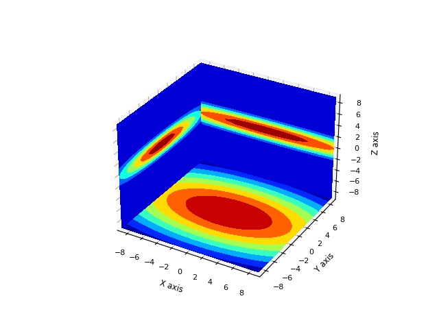
- jscatter.mpl.contourOnCube(xy, yz=None, xz=None, shape=None, offset=None, levels=None, colorMap='jet', scale='norm', block=False, linthresh=1, linscale=1, badcolor=None, ax=None)[source]
Plot 3 2d contourf planes on surface of a cube.
Intended to show 3D perpendicular scattering planes together.
- Parameters:
- xy,yz,xzarray 3xNM
2D data [x,y,z] with shape N*M = NM. Each is ploted parallel to the plane mentioned in name. regrid is used to reshape to dimension 3xNxM
- shapelist 2x float
2D shape of the above arrays
- offsetlist 3x float, default 0,0,0
Position of the xy,yz,xz planes in a 3D plot.
- levelsint, None, sequence of values
Number of contour lines between min and max or sequence of specific values.
- colorMapstring
Get a colormap instance from name. Standard mpl colormap name (see showColors).
- badcolorfloat, color
Set the color for bad values (like masked pixel) values in an image. Default is bad values be transparent. Color can be matplotlib color as ‘k’,’b’ or float value in interval [0,1] of the chosen colorMap. 0 sets to minimum value, 1 to maximum value.
- scale‘log’, ‘symlog’, default = ‘norm’
Scale for intensities.
‘norm’ Linear scale.
‘log’ Logarithmic scale
‘symlog’ Symmetrical logarithmic scale is logarithmic in both the positive and negative directions from the origin. This works also for only positive data. Use linthresh, linscale to adjust.
- linthreshfloat, default = 1
Only used for scale ‘sym’. The range within which the plot is linear (-linthresh to linthresh).
- linscalefloat, default = 1
Only used for scale ‘sym’. Its value is the number of decades to use for each half of the linear range. E.g. 10 uses 1 decade.
- blockbool
Open in blocking or non-blocking mode
- axfigure axes, default None
Axes to plot inside. If None a new Figure is opened.
- Returns:
- axes
Examples
%matplotlib
import jscatter as js
import numpy as np

# detector planes; a real flat detector has z>0
q = np.mgrid[-9:9:51j, -9:9:51j].reshape(2,-1).T
grid= js.sf.scLattice(10/20,20).XYZ
fa = js.cloudscattering.fa_cuboid(*grid[:,:3].T,0.2,0.4,2)

rod0=np.array([[0,0,0,1,0,0]])
qz=np.c_[q,np.zeros_like(q[:,0])]  # for z=0
qy=np.c_[q[:,:1],np.zeros_like(q[:,0]),q[:,1:]]  # for z=0
qx=np.c_[np.zeros_like(q[:,0]),q]  # for z=0

ffz1 = js.ff.orientedCloudScattering3Dff(qz,cloud=rod0, formfactoramp=fa)
ffy1 = js.ff.orientedCloudScattering3Dff(qy,cloud=rod0, formfactoramp=fa)
ffx1 = js.ff.orientedCloudScattering3Dff(qx,cloud=rod0, formfactoramp=fa)

# show as cube surfaces
ax=js.mpl.contourOnCube(ffz1[[0,1,3]].array,ffx1[[1,2,3]].array,ffy1[[0,2,3]].array,offset=[-9,-9,9])
#ax.figure.savefig(js.examples.imagepath+'/contourOnCube.jpg')
- jscatter.mpl.showColors()[source]
Get a list of the colormaps in matplotlib.
Ignore the ones that end with ‘_r’ because these are simply reversed versions of ones that don’t end with ‘_r’
- Colormaps Names
Accent, Accent_r, Blues, Blues_r, BrBG, BrBG_r, BuGn, BuGn_r, BuPu, BuPu_r, CMRmap, CMRmap_r, Dark2, Dark2_r, GnBu, GnBu_r, Greens, Greens_r, Greys, Greys_r, OrRd, OrRd_r, Oranges, Oranges_r, PRGn, PRGn_r, Paired, Paired_r, Pastel1, Pastel1_r, Pastel2, Pastel2_r, PiYG, PiYG_r, PuBu, PuBuGn, PuBuGn_r, PuBu_r, PuOr, PuOr_r, PuRd, PuRd_r, Purples, Purples_r, RdBu, RdBu_r, RdGy, RdGy_r, RdPu, RdPu_r, RdYlBu, RdYlBu_r, RdYlGn, RdYlGn_r, Reds, Reds_r, Set1, Set1_r, Set2, Set2_r, Set3, Set3_r, Spectral, Spectral_r, Vega10, Vega10_r, Vega20, Vega20_r, Vega20b, Vega20b_r, Vega20c, Vega20c_r, Wistia, Wistia_r, YlGn, YlGnBu, YlGnBu_r, YlGn_r, YlOrBr, YlOrBr_r, YlOrRd, YlOrRd_r, afmhot, afmhot_r, autumn, autumn_r, binary, binary_r, bone, bone_r, brg, brg_r, bwr, bwr_r, cool, cool_r, coolwarm, coolwarm_r, copper, copper_r, cubehelix, cubehelix_r, flag, flag_r, gist_earth, gist_earth_r, gist_gray, gist_gray_r, gist_heat, gist_heat_r, gist_ncar, gist_ncar_r, gist_rainbow, gist_rainbow_r, gist_stern, gist_stern_r, gist_yarg, gist_yarg_r, gnuplot, gnuplot2, gnuplot2_r, gnuplot_r, gray, gray_r, hot, hot_r, hsv, hsv_r, inferno, inferno_r, jet, jet_r, magma, magma_r, nipy_spectral, nipy_spectral_r, ocean, ocean_r, pink, pink_r, plasma, plasma_r, prism, prism_r, rainbow, rainbow_r, seismic, seismic_r, spectral, spectral_r, spring, spring_r, summer, summer_r, tab10, tab10_r, tab20, tab20_r, tab20b, tab20b_r, tab20c, tab20c_r, terrain, terrain_r, viridis, viridis_r, winter, winter_r
From https://matplotlib.org/1.2.1/examples/pylab_examples/show_colormaps.html
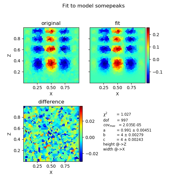
- jscatter.mpl.showlastErrPlot2D(data, lastfit=None, shape=None, scale='norm', colorMap='jet', method='nearest', linthresh=1, linscale=1, badcolor=None, transpose=None, figsize=[6, 6], txtkwargs={'fontsize': 'small'})[source]
Show a 2D errplot for 2D fit data.
- Parameters:
- datadataArray
dataArray optional with fit values in lastfit.
- lastfitNone, dataArray
Lastfit dataArray if not present in data. Can be used to create showlastErrPlot2D from saved data and lastfit.
- shape[int,int]
Optional shape of the data if these are from an image. If not given the data are interpolated (regrid)
- methodfloat,’linear’, ‘nearest’, ‘cubic’
Filling value for new points as float or order of interpolation between existing points. See griddata
- colorMapstring
Get a colormap instance from name. Standard mpl colormap name (see showColors).
- badcolorfloat, color
Set the color for bad values (like masked pixel) values in an image. Default is bad values be transparent. Color can be matplotlib color as ‘k’,’b’ or float value in interval [0,1] of the chosen colorMap. 0 sets to minimum value, 1 to maximum value.
- scale‘log’, ‘symlog’, default = ‘norm’
Scale for intensities.
‘norm’ Linear scale.
‘log’ Logarithmic scale
‘symlog’ Symmetrical logarithmic scale is logarithmic in both the positive and negative directions from the origin. This works also for only positive data. Use linthresh, linscale to adjust.
- linthreshfloat, default = 1
Only used for scale ‘sym’. The range within which the plot is linear (-linthresh to linthresh).
- linscalefloat, default = 1
Only used for scale ‘sym’. Its value is the number of decades to use for each half of the linear range. E.g. 10 uses 1 decade.
- transposebool
Transpose coordinates, e.g. for sasImages.
- figsize[float,float], default [6,6]
Figure Size in inch.
- txtkwargskwargs
Keyword arguments passed to Text https://matplotlib.org/api/text_api.html#matplotlib.text.Text). except x,y,text arguments.
Examples
%matplotlib
import jscatter as js
import numpy as np
# create 2D data with X,Z axes and Y values as Y=f(X,Z)
x,z=np.mgrid[-5:3:0.05,-5:9:0.05]
xyz=js.dA(np.c_[x.flatten(),
               z.flatten(),
               0.3*np.sin(x*z/np.pi).flatten()+0.01*np.random.randn(len(x.flatten())),
               0.01*np.ones_like(x).flatten() ].T)
# set columns where to find X,Y,Z )
xyz.setColumnIndex(ix=0,iz=1,iy=2,iey=3)
#
ff=lambda x,z,a,b:a*np.sin(b*x*z)
xyz.fit(ff,{'a':1,'b':1/3.},{},{'x':'X','z':'Z'})
fig = js.mpl.showlastErrPlot2D(xyz)
#fig.savefig(js.examples.imagepath+'/2dfitgoodfit2.jpg')
xyz.save('dat.dat')  # save data
xyz.lastfit.save('lastfit.dat')  # save lastfit
# recover from saved data above
fig = js.mpl.showlastErrPlot2D(js.dA('dat.dat'),js.dA('lastfit.dat'))

%matplotlib
import jscatter as js
import numpy as np
import matplotlib.pyplot as pyplot
import matplotlib.tri as tri
randn=np.random.randn
rand=np.random.rand
def somepeaks(width, height,a,b,c):
    return a*width*(1-width)*np.cos(b*np.pi*width) * np.sin(c*np.pi*height**2)**2

# create random points in [0,1]
NN=1000
xz = rand(NN, 2)
v = somepeaks(xz[:,0], xz[:,1],1,4,4)
# create dataArray
data=js.dA(np.stack([xz[:,0], xz[:,1],v+0.01*randn(NN),np.ones(NN)*0.01]), XYeYeX=[0, 2, 3, None, 1, None])
# bad start parameters
data.fit(somepeaks,{'a':1,'b':2,'c':1},{},{'width':'X','height':'Z'})
fig = js.mpl.showlastErrPlot2D(data)
# good start parameters
data.fit(somepeaks,{'a':0.8,'b':3.8,'c':4.2},{},{'width':'X','height':'Z'})
fig = js.mpl.showlastErrPlot2D(data)
#fig.savefig(js.examples.imagepath+'/2dfitgoodfit.jpg')
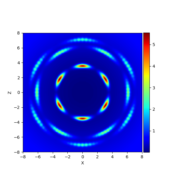
- jscatter.mpl.plot2Dimage(data, shape=None, yaxis_label='Z', xaxis_label='X', method='nearest', colorMap='jet', scale='norm', linthresh=1, linscale=1, badcolor=None, transpose=None, figsize=[6, 6], origin='upper', txtkwargs={'fontsize': 'small'}, ax=None)[source]
Show a 2D image of a dataarray with XZW values like from oriented cloudscattering.
- Parameters:
- datadataArray
dataArray optional with fit values in lastfit.
- shape[int,int]
Optional shape of the data if these are from an image. If not given the data are interpolated (regrid)
- yaxis_labelstring
- xaxis_labelstring
- methodfloat,’linear’, ‘nearest’, ‘cubic’
Filling value for new points as float or order of interpolation between existing points. See griddata
- colorMapstring
Get a colormap instance from name. Standard mpl colormap name (see showColors).
- scale‘log’, ‘symlog’, default = ‘norm’
Scale for intensities.
‘norm’ Linear scale.
‘log’ Logarithmic scale
‘symlog’ Symmetrical logarithmic scale is logarithmic in both the positive and negative directions from the origin. This works also for only positive data. Use linthresh, linscale to adjust.
- linthreshfloat, default = 1
Only used for scale ‘sym’. The range within which the plot is linear (-linthresh to linthresh).
- linscalefloat, default = 1
Only used for scale ‘sym’. Its value is the number of decades to use for each half of the linear range. E.g. 10 uses 1 decade.
- badcolorfloat, color
Set the color for bad values (like masked pixel) values in an image. Default is bad values be transparent. Color can be matplotlib color as ‘k’,’b’ or float value in interval [0,1] of the chosen colorMap. 0 sets to minimum value, 1 to maximum value.
- transposebool
Transpose coordinates, e.g. for sasImages.
- figsize[float,float], default [6,6]
Figure Size in inch.
- txtkwargskwargs
Keyword arguments passed to Text https://matplotlib.org/api/text_api.html#matplotlib.text.Text). except x,y,text arguments.
- axfigure axes, default None
Axes to plot inside. If None a new Figure is opened.
- Returns:
- figure
Examples
%matplotlib
import jscatter as js
import numpy as np

R=8    # maximum
N=200  # number of points
ds=15;
qxy=np.mgrid[-R:R:N*1j, -R:R:N*1j].reshape(2,-1).T
# add z=0 component
qxyz=np.c_[qxy,np.zeros(qxy.shape[0])].T # as position vectors
# create fcc lattice which includes reciprocal lattice vectors and methods to get peak positions
fcclattice= js.lattice.fccLattice(5, 5)
# Orient 111 direction perpendicular to qxy plane
fcclattice.rotatehkl2Vector([1,1,1],[0,0,1])
# rotation by 15 degrees to be aligned to xy plane
fcclattice.rotateAroundhkl([1,1,1],np.deg2rad(-15))
ffs=js.sf.orientedLatticeStructureFactor(qxyz,fcclattice, rotation=[1,1,1,np.deg2rad(10)],
                           domainsize=ds,rmsd=0.1,hklmax=5,nGauss=23)

js.mpl.plot2Dimage(ffs)
- jscatter.mpl.test(keepopen=True)[source]
A small test for mpl module making a plot.
Run as
js.mpl.test()Examples
For interactive plots in Ipython the event loop needs to be defined by calling %matplotlib
%matplotlib
import jscatter as js
import numpy as np
from matplotlib import pyplot
# use this
#fig=pyplot.figure(FigureClass=js.mpl.Figure)
# or
fig=js.mplot()
fig.Multi(2,1)
fig[0].SetView(0.1,0.25,0.8,0.9)
fig[1].SetView(0.1,0.09,0.8,0.23)
q=js.loglist(0.01,5,100)
aa=js.dL()
for pp in range(5):
    aa.append(js.dA(np.c_[q,-pp*np.sin(q),0.2*np.cos(5*q)].T))
    aa[-1].qq=pp
bb=js.dA(np.c_[q,q**2].T)
bb.qq=123
for pp in range(5):
    fig[0].Plot(aa[pp].X,-1*aa[pp].Y,legend='some stufff',sy=[1,(pp+1)/10.],li=0)

fig[0].Plot(aa, legend='qq = $qq', sy=[-1, 0.4, -1, ''], li=0, markeredgewidth=1)
for pp in range(5):
    fig[1].Plot(aa[-1].X/5+pp,pp*aa[-1].Y,legend='q=%.1f' %pp,sy=0,li=-1,markeredgewidth =1)
fig[1].Plot(bb,legend='sqr=$qq ',sy=2,li=2)
fig[0].Title('test')
fig[0].Legend(x=1.3,y=1)
fig[1].Legend(x=1.3,y=1)
fig[0].Yaxis(label='y-axis')
fig[1].Yaxis(label='something else')
fig[0].tick_params(labelbottom=False)
fig[1].Xaxis(label='x-axis')

# plot with a given size and dpi (3.25 inch JACS column width)
fig.set_size_inches(3.25*2, 2*2)
fig.savefig("sample.png", dpi=100)  # with 300dpi results in 600dpi
11.2.1. Matplotlib figures
|
Open matplotlib figure in paper layout with figure/axes methods to display dataArray/dataList. |
|
Surface plot of x,y,z, data |
|
Scatter plot of x,y,z data points. |
|
Image with contour lines of 3D dataArrays or sasImage/image array. |
|
Show a 2D image of a dataarray with XZW values like from oriented cloudscattering. |
Get a list of the colormaps in matplotlib. |
|
|
Plot 3 2d contourf planes on surface of a cube. |
|
Show a 2D errplot for 2D fit data. |
|
A small test for mpl module making a plot. |
11.2.2. Figure Methods
|
Creates multiple subplots on grid n,m. |
|
Add a subplot in the foreground using jscatter paper default layout. |
|
|
|
Clear content of all axes |
|
Save with filename |
|
Is the figure window still open. |
|
11.2.3. Axes Methods
|
Plot dataArrays/dataList or array in matplotlib axes. |
|
Set xaxis |
|
Set xaxis |
|
Show/update legend. |
|
set figure title |
|
Append subtitle to title |
|
This sets the bounding box of the axes. |
|
Clear data of this axes. |
|
|
|
Plot an arrow or line. |
This is a rudimentary interface to matplotlib to use dataArrays/sasImage easier. The standard way to use matplotlib is full available without using this module and recommended for more complicated use cases. Nevertheless, the source can be used as template to be adapted.
The intention is to allow fast/easy plotting (one command to plot) with some convenience function in relation to dataArrays and in a non-blocking mode of matplotlib. E.g. to include automatically the value of an attribute (qq in example) in the legend for daily work and inspection of your data
fig = js.mplot()
fig[0].Plot(mydataArray, legend='sqr=$qq',sy=[2,3,-1], li=0)
fig[0].Plot(mydataList , legend='sqr=$qq',sy=[2,3,-1], li=0)
We have some shortcuts to determine the marker (sy=symbol) and line (li) and legend (le). Matplotlib is quite slow, for faster 2D plotting use xmgrace (e.g. updates during fits are much faster). For 3D plotting we have some simple plot functions to get a result in one line.
js.usempl(True)switches to mpl in fitting and examples.The new methods introduced all start with a big Letter to allow still the access of the original matplotlib methods.
By indexing subplots can be accessed as figure[i] which is figure.axes[i].
Same for axes with lines figure[0][i] is figure.axes[0].lines[i].
The
axoption of later commands allows to plot in a multi plot.
Example 1 For interactive plots in Ipython the event loop needs to be defined by calling %matplotlib
%matplotlib
import jscatter as js
import numpy as np

# get some data
i5=js.dL(js.examples.datapath+'/iqt_1hho.dat')
x,z=np.mgrid[-4:8:0.1,-3:5:0.1]
xyz=js.dA(np.c_[x.flatten(),z.flatten(),0.3*np.sin(x*z/np.pi).flatten()].T)
xyz.setColumnIndex(ix=0,iy=2,iz=1)

# plot it
p=js.mplot(20,10)  # with size in cm
p.Multi(1,2)
p[0].Plot(i5,sy=[-1,0.2,-1,-1],li=1,legend='Q= $q')
js.mpl.contourImage(xyz,invert_yaxis=True,ax=p[1])

# pretty up for paper or presentation
p[0].Yaxis(scale='l',max=1.1,min=0.05)
p[0].Title('Some unrelated data')
p[0].Legend(x=1.43,y=1,charsize=0.8) # x,y in relative units of the plot
p[0].Yaxis(label='I(Q,t)/I(Q,0)',min=0.01)
p[0].Xaxis(label='Q / 1/nm',max=120)

# p.savefig(js.examples.imagepath+'/lineandcontourImage.jpg', dpi=100)
Save in given size and resolution, e.g. 3.25 inch JACS column width with 600 dpi
# the factor 3 is only to get a reasonable screen size with reasonable char sizes
p.set_size_inches(3.25*3, 1.6*3)
p.savefig('lineandcontourImage.jpg', dpi=200)
See another Example test()
Some short hints for matplotlib
Dont use the pyplot interface as it hides how most things work and e.g. how to access lines later.
See THIS .
After fitting the errorplot can be accessed as data.errplot.
fig=js.mplot()                         # access figure properties from fig
fig.axes[0]                            # access to axes properties first axes
fig.axes[1].lines[3]                   # access properties of 3rd line in axes 1
fig.axes[0].lines[1].set_color('b')    # change color
fig.axes[0].legend(...)                # set legend
data.errplot.axes[0].set_yscale('log') # set log scale in errplot
# for more read matplotlib documentation for object oriented access
- jscatter.mpl.is_terminal() bool[source]
Detect if Python is running in a terminal. Returns True if Python is running in a terminal or False if not.
- jscatter.mpl.gf = 20
gracefactor to get same scaling as in grace set to 10
- class jscatter.mpl.jspaperAxes(*args, **kwargs)[source]
Bases:
AxesBuild an Axes in a figure.
- Parameters:
- fig~matplotlib.figure.Figure
The Axes is built in the .Figure fig.
- *args
*argscan be a single(left, bottom, width, height)rectangle or a single .Bbox. This specifies the rectangle (in figure coordinates) where the Axes is positioned.*argscan also consist of three numbers or a single three-digit number; in the latter case, the digits are considered as independent numbers. The numbers are interpreted as(nrows, ncols, index):(nrows, ncols)specifies the size of an array of subplots, andindexis the 1-based index of the subplot being created. Finally,*argscan also directly be a .SubplotSpec instance.- sharex, sharey~matplotlib.axes.Axes, optional
The x- or y-~.matplotlib.axis is shared with the x- or y-axis in the input ~.axes.Axes. Note that it is not possible to unshare axes.
- frameonbool, default: True
Whether the Axes frame is visible.
- box_aspectfloat, optional
Set a fixed aspect for the Axes box, i.e. the ratio of height to width. See ~.axes.Axes.set_box_aspect for details.
- forward_navigation_eventsbool or “auto”, default: “auto”
Control whether pan/zoom events are passed through to Axes below this one. “auto” is True for axes with an invisible patch and False otherwise.
- **kwargs
Other optional keyword arguments:
Properties: adjustable: {‘box’, ‘datalim’} agg_filter: a filter function, which takes a (m, n, 3) float array and a dpi value, and returns a (m, n, 3) array and two offsets from the bottom left corner of the image alpha: float or None anchor: (float, float) or {‘C’, ‘SW’, ‘S’, ‘SE’, ‘E’, ‘NE’, …} animated: bool aspect: {‘auto’, ‘equal’} or float autoscale_on: bool autoscalex_on: unknown autoscaley_on: unknown axes_locator: Callable[[Axes, Renderer], Bbox] axisbelow: bool or ‘line’ box_aspect: float or None clip_box: ~matplotlib.transforms.BboxBase or None clip_on: bool clip_path: Patch or (Path, Transform) or None facecolor or fc: :mpltype:`color` figure: ~matplotlib.figure.Figure or ~matplotlib.figure.SubFigure forward_navigation_events: bool or “auto” frame_on: bool gid: str in_layout: bool label: object mouseover: bool navigate: bool navigate_mode: unknown path_effects: list of .AbstractPathEffect picker: None or bool or float or callable position: [left, bottom, width, height] or ~matplotlib.transforms.Bbox prop_cycle: ~cycler.Cycler rasterization_zorder: float or None rasterized: bool sketch_params: (scale: float, length: float, randomness: float) snap: bool or None subplotspec: unknown title: str transform: ~matplotlib.transforms.Transform url: str visible: bool xbound: (lower: float, upper: float) xinverted: unknown xlabel: str xlim: (left: float, right: float) xmargin: float greater than -0.5 xscale: unknown xticklabels: unknown xticks: unknown ybound: (lower: float, upper: float) yinverted: unknown ylabel: str ylim: (bottom: float, top: float) ymargin: float greater than -0.5 yscale: unknown yticklabels: unknown yticks: unknown zorder: float
- Returns:
- ~.axes.Axes
The new ~.axes.Axes object.
- name = 'paper'
- SetView(xmin=None, ymin=None, xmax=None, ymax=None)[source]
This sets the bounding box of the axes.
- Parameters:
- xmin,xmax,ymin,ymaxfloat
view range
- plot(*datasets, **kwargs)[source]
Plot dataArrays/dataList or array in matplotlib axes.
Parameters are passed to matplotlib.axes.Axes.plot
- Parameters:
- datasetsdataArray/dataList or 1D arrays
- Datasets to plot.
Can be several dataArray/dataList (with .X, .Y and .eY) or 1D arrays (a[1,:],b[2,:]), but don’t mix it.
If dataArray/dataList has .eY errors a errorbars are plotted.
If format strings are found only the first is used. symbol, line override this.
Only a single line for 1D arrays is allowed.
- symbol,syint, list of float
[symbol,size,color,fillcolor,fillpattern] as [1,1,1,-1];
single integer to chose symbol e.g.symbol=3; symbol=0 switches off
negative increments from last
symbol => see Line2D.filled_markers
size => size in pixel
color => int in sequence = wbgrcmyk
fillcolor=None see color
fillpattern=None 0 empty, 1 full, ….test it
- line,liint, list of float or Line object
[linestyle,linewidth,color] as [1,1,’’];
negative increments
single integer to chose linestyle line=1; line=0 switches of
linestyle int ‘-‘,’–‘,’-.’,’:’
linewidth float increasing thickness
color see symbol color
- errorbar,erint or list of float or Errorbar object
[color,size] as [1,1]; no increment, no repeat
color int see symbol color, non-integer syncs to symbol color
size float default 1.0 ; smaller is 0.5
- legend,lestring
determines legend for all datasets
string replacement: attr name prepended by ‘$’ (eg. ‘$par’) is replaced by value str(par1.flatten()[0]) if possible. $(par) for not unique names
- errorbar,erfloat
errorbar thickness, zero is no errorbar
- Plot(*datasets, **kwargs)
Plot dataArrays/dataList or array in matplotlib axes.
Parameters are passed to matplotlib.axes.Axes.plot
- Parameters:
- datasetsdataArray/dataList or 1D arrays
- Datasets to plot.
Can be several dataArray/dataList (with .X, .Y and .eY) or 1D arrays (a[1,:],b[2,:]), but don’t mix it.
If dataArray/dataList has .eY errors a errorbars are plotted.
If format strings are found only the first is used. symbol, line override this.
Only a single line for 1D arrays is allowed.
- symbol,syint, list of float
[symbol,size,color,fillcolor,fillpattern] as [1,1,1,-1];
single integer to chose symbol e.g.symbol=3; symbol=0 switches off
negative increments from last
symbol => see Line2D.filled_markers
size => size in pixel
color => int in sequence = wbgrcmyk
fillcolor=None see color
fillpattern=None 0 empty, 1 full, ….test it
- line,liint, list of float or Line object
[linestyle,linewidth,color] as [1,1,’’];
negative increments
single integer to chose linestyle line=1; line=0 switches of
linestyle int ‘-‘,’–‘,’-.’,’:’
linewidth float increasing thickness
color see symbol color
- errorbar,erint or list of float or Errorbar object
[color,size] as [1,1]; no increment, no repeat
color int see symbol color, non-integer syncs to symbol color
size float default 1.0 ; smaller is 0.5
- legend,lestring
determines legend for all datasets
string replacement: attr name prepended by ‘$’ (eg. ‘$par’) is replaced by value str(par1.flatten()[0]) if possible. $(par) for not unique names
- errorbar,erfloat
errorbar thickness, zero is no errorbar
- Yaxis(min=None, max=None, label=None, scale=None, size=None, charsize=None, tick=None, ticklabel=None, **kwargs)[source]
Set xaxis
- Parameters:
- labelstring
Label
- scale‘log’, ‘normal’
Scale
- min,maxfloat
Set min and max
- sizeint
Pixelsize of label
- Xaxis(min=None, max=None, label=None, scale=None, size=None, charsize=None, tick=None, ticklabel=None, **kwargs)[source]
Set xaxis
- Parameters:
- labelstring
Label
- scale‘log’, ‘normal’
Scale
- min,maxfloat
Set min and max of scale
- sizeint
Pixelsize of label
- Legend(**kwargs)[source]
Show/update legend.
- Parameters:
- charsize, fontsizeint, default 12
Font size of labels
- labelspacingint , default =12
Spacing of labels
- locint [0..10] default 1 ‘upper right’
Location specifier - ‘best’ 0, ‘upper right’ 1, ‘upper left’ 2, ‘lower left’ 3, ‘lower right’ 4,‘center left’ 6,
- x,yfloat [0..1]
Determines, if both given, loc and sets position in axes coordinates. Sets bbox_to_anchor=(x,y). Values outside [0,1] are ignored.
- kwargskwargs of axes.legend
Any given kwarg overrides the previous
- Arrow(x1=None, y1=None, x2=None, y2=None, linewidth=None, arrow=None)[source]
Plot an arrow or line.
- Parameters:
- x1,y1,x2,y2float
Start/end coordinates in box units [0..1].
- linewidthfloat
Linewidth
- arrowint or [‘-‘,’->’,’<-‘,’<->’]
Type of arrow. If int it selects from [‘-‘,’->’,’<-‘,’<->’]
- Returns:
- set(*, adjustable=<UNSET>, agg_filter=<UNSET>, alpha=<UNSET>, anchor=<UNSET>, animated=<UNSET>, aspect=<UNSET>, autoscale_on=<UNSET>, autoscalex_on=<UNSET>, autoscaley_on=<UNSET>, axes_locator=<UNSET>, axisbelow=<UNSET>, box_aspect=<UNSET>, clip_box=<UNSET>, clip_on=<UNSET>, clip_path=<UNSET>, facecolor=<UNSET>, forward_navigation_events=<UNSET>, frame_on=<UNSET>, gid=<UNSET>, in_layout=<UNSET>, label=<UNSET>, mouseover=<UNSET>, navigate=<UNSET>, path_effects=<UNSET>, picker=<UNSET>, position=<UNSET>, prop_cycle=<UNSET>, rasterization_zorder=<UNSET>, rasterized=<UNSET>, sketch_params=<UNSET>, snap=<UNSET>, subplotspec=<UNSET>, title=<UNSET>, transform=<UNSET>, url=<UNSET>, visible=<UNSET>, xbound=<UNSET>, xinverted=<UNSET>, xlabel=<UNSET>, xlim=<UNSET>, xmargin=<UNSET>, xscale=<UNSET>, xticklabels=<UNSET>, xticks=<UNSET>, ybound=<UNSET>, yinverted=<UNSET>, ylabel=<UNSET>, ylim=<UNSET>, ymargin=<UNSET>, yscale=<UNSET>, yticklabels=<UNSET>, yticks=<UNSET>, zorder=<UNSET>)
Set multiple properties at once.
a.set(a=A, b=B, c=C)
is equivalent to
a.set_a(A)
a.set_b(B)
a.set_c(C)
In addition to the full property names, aliases are also supported, e.g.
set(lw=2)is equivalent toset(linewidth=2), but it is an error to pass both simultaneously.The order of the individual setter calls matches the order of parameters in
set(). However, most properties do not depend on each other so that order is rarely relevant.Supported properties are
- Properties:
adjustable: {‘box’, ‘datalim’} agg_filter: a filter function, which takes a (m, n, 3) float array and a dpi value, and returns a (m, n, 3) array and two offsets from the bottom left corner of the image alpha: float or None anchor: (float, float) or {‘C’, ‘SW’, ‘S’, ‘SE’, ‘E’, ‘NE’, …} animated: bool aspect: {‘auto’, ‘equal’} or float autoscale_on: bool autoscalex_on: unknown autoscaley_on: unknown axes_locator: Callable[[Axes, Renderer], Bbox] axisbelow: bool or ‘line’ box_aspect: float or None clip_box: ~matplotlib.transforms.BboxBase or None clip_on: bool clip_path: Patch or (Path, Transform) or None facecolor or fc: :mpltype:`color` figure: ~matplotlib.figure.Figure or ~matplotlib.figure.SubFigure forward_navigation_events: bool or “auto” frame_on: bool gid: str in_layout: bool label: object mouseover: bool navigate: bool navigate_mode: unknown path_effects: list of .AbstractPathEffect picker: None or bool or float or callable position: [left, bottom, width, height] or ~matplotlib.transforms.Bbox prop_cycle: ~cycler.Cycler rasterization_zorder: float or None rasterized: bool sketch_params: (scale: float, length: float, randomness: float) snap: bool or None subplotspec: unknown title: str transform: ~matplotlib.transforms.Transform url: str visible: bool xbound: (lower: float, upper: float) xinverted: unknown xlabel: str xlim: (left: float, right: float) xmargin: float greater than -0.5 xscale: unknown xticklabels: unknown xticks: unknown ybound: (lower: float, upper: float) yinverted: unknown ylabel: str ylim: (bottom: float, top: float) ymargin: float greater than -0.5 yscale: unknown yticklabels: unknown yticks: unknown zorder: float
- dataLim: mtransforms.Bbox
The bounding .Bbox enclosing all data displayed in the Axes.
- spines: mspines.Spines
The .Spines container for the Axes’ spines, i.e. the lines denoting the data area boundaries.
- xaxis: maxis.XAxis
The .XAxis instance.
Common axis-related configuration can be achieved through high-level wrapper methods on Axes; e.g. ax.set_xticks <.Axes.set_xticks> is a shortcut for ax.xaxis.set_ticks <.Axis.set_ticks>. The xaxis attribute gives direct direct access to the underlying ~.axis.Axis if you need more control.
See also
Axis wrapper methods on Axes
Axis API
- yaxis: maxis.YAxis
The .YAxis instance.
Common axis-related configuration can be achieved through high-level wrapper methods on Axes; e.g. ax.set_yticks <.Axes.set_yticks> is a shortcut for ax.yaxis.set_ticks <.Axis.set_ticks>. The yaxis attribute gives direct access to the underlying ~.axis.Axis if you need more control.
See also
Axis wrapper methods on Axes
Axis API
- class jscatter.mpl.jsFigure(*args, **kwargs)[source]
Bases:
FigureCreate figure with Axes as jspaperAxes projection.
This is used from mplot and should not be called directly.
Examples
%matplotlib
import jscatter as js
import numpy as np
i5=js.dL(js.examples.datapath+'/iqt_1hho.dat')
p=js.mplot()
p[0].Plot(i5,sy=[-1,0.4,-1],li=1,legend='Q= $q')
p[0].Yaxis(scale='l')
p[0].Title('intermediate scattering function')
p[0].Legend(x=1.13,y=1) # x,y in relative units of the plot
p[0].Yaxis(label='I(Q,t)/I(Q,0)',min=0.01, max=1.1)
p[0].Xaxis(label='Q / 1/nm',min=0,max=120)
- Multi(n, m)[source]
Creates multiple subplots on grid n,m. with projection “jspaperAxes”.
Subplots can be accesses as fig[i]
- Addsubplot(bbox=(0.2, 0.2, 0.6, 0.6), *args, **kwargs)[source]
Add a subplot in the foreground using jscatter paper default layout.
To use matplotlib default use add_subplot.
To change order of drawing (stacking) use the zorder attribute as fig.axes[1].set_zorder(3)
- Parameters:
- bboxrect [left, bottom, width, height]
Bounding box position and size.
- args,kwargs
See all arguments for matplotlib subplot except projection.
Examples
- ::
%matplotlib import jscatter as js fig=js.mplot() fig.Addsubplot() # a default position (dont repeat same positions) fig.Addsubplot([0.3,0.3,0.3,0.3])
- Save(filename, format=None, dpi=None, **kwargs)[source]
Save with filename
Same options as matplotlib savefig.
- Plot(*args, **kwargs)
- show(*args, **kwargs)[source]
If using a GUI backend with pyplot, display the figure window.
If the figure was not created using ~.pyplot.figure, it will lack a ~.backend_bases.FigureManagerBase, and this method will raise an AttributeError.
Warning
This does not manage a GUI event loop. Consequently, the figure may only be shown briefly or not shown at all if you or your environment are not managing an event loop.
Use cases for .Figure.show include running this from a GUI application (where there is persistently an event loop running) or from a shell, like IPython, that install an input hook to allow the interactive shell to accept input while the figure is also being shown and interactive. Some, but not all, GUI toolkits will register an input hook on import. See cp_integration for more details.
If you’re in a shell without input hook integration or executing a python script, you should use matplotlib.pyplot.show with
block=Trueinstead, which takes care of starting and running the event loop for you.- Parameters:
- warnbool, default: True
If
Trueand we are not running headless (i.e. on Linux with an unset DISPLAY), issue warning when called on a non-GUI backend.
- Show(*args, **kwargs)
If using a GUI backend with pyplot, display the figure window.
If the figure was not created using ~.pyplot.figure, it will lack a ~.backend_bases.FigureManagerBase, and this method will raise an AttributeError.
Warning
This does not manage a GUI event loop. Consequently, the figure may only be shown briefly or not shown at all if you or your environment are not managing an event loop.
Use cases for .Figure.show include running this from a GUI application (where there is persistently an event loop running) or from a shell, like IPython, that install an input hook to allow the interactive shell to accept input while the figure is also being shown and interactive. Some, but not all, GUI toolkits will register an input hook on import. See cp_integration for more details.
If you’re in a shell without input hook integration or executing a python script, you should use matplotlib.pyplot.show with
block=Trueinstead, which takes care of starting and running the event loop for you.- Parameters:
- warnbool, default: True
If
Trueand we are not running headless (i.e. on Linux with an unset DISPLAY), issue warning when called on a non-GUI backend.
- set(*, agg_filter=<UNSET>, alpha=<UNSET>, animated=<UNSET>, canvas=<UNSET>, clip_box=<UNSET>, clip_on=<UNSET>, clip_path=<UNSET>, constrained_layout=<UNSET>, constrained_layout_pads=<UNSET>, dpi=<UNSET>, edgecolor=<UNSET>, facecolor=<UNSET>, figheight=<UNSET>, figwidth=<UNSET>, frameon=<UNSET>, gid=<UNSET>, in_layout=<UNSET>, label=<UNSET>, layout_engine=<UNSET>, linewidth=<UNSET>, mouseover=<UNSET>, path_effects=<UNSET>, picker=<UNSET>, rasterized=<UNSET>, size_inches=<UNSET>, sketch_params=<UNSET>, snap=<UNSET>, tight_layout=<UNSET>, transform=<UNSET>, url=<UNSET>, visible=<UNSET>, zorder=<UNSET>)
Set multiple properties at once.
a.set(a=A, b=B, c=C)
is equivalent to
a.set_a(A)
a.set_b(B)
a.set_c(C)
In addition to the full property names, aliases are also supported, e.g.
set(lw=2)is equivalent toset(linewidth=2), but it is an error to pass both simultaneously.The order of the individual setter calls matches the order of parameters in
set(). However, most properties do not depend on each other so that order is rarely relevant.Supported properties are
- Properties:
agg_filter: a filter function, which takes a (m, n, 3) float array and a dpi value, and returns a (m, n, 3) array and two offsets from the bottom left corner of the image alpha: float or None animated: bool canvas: FigureCanvas clip_box: ~matplotlib.transforms.BboxBase or None clip_on: bool clip_path: Patch or (Path, Transform) or None constrained_layout: unknown constrained_layout_pads: unknown dpi: float edgecolor: :mpltype:`color` facecolor: :mpltype:`color` figheight: float figure: unknown figwidth: float frameon: bool gid: str in_layout: bool label: object layout_engine: {‘constrained’, ‘compressed’, ‘tight’, ‘none’, .LayoutEngine, None} linewidth: number mouseover: bool path_effects: list of .AbstractPathEffect picker: None or bool or float or callable rasterized: bool size_inches: (float, float) or float sketch_params: (scale: float, length: float, randomness: float) snap: bool or None tight_layout: unknown transform: ~matplotlib.transforms.Transform url: str visible: bool zorder: float
- jscatter.mpl.show(**kwargs)[source]
Updates figures or saves figures in noninteractive mode (headless)
In headless mode all figures are save to lastopenedplots{i}.png .
- Parameters:
- kwargsargs
Passed to pyplot.show added by block=False
- jscatter.mpl.mplot(width=None, height=None, **kwargs)[source]
Open matplotlib figure in paper layout with figure/axes methods to display dataArray/dataList.
Paper layout means white background, black axis. Plot separates X,Y, eY of dataList automatically. In interactive mode the figure is shown, in headless these can be saved after plotting.
- Parameters:
- width,heightfloat
Size of plot in cm.
- kwargs
Keyword args of matplotlib.pyplot.figure .
- Returns:
- matplotlib figure
Notes
By indexing as the axes subplots can be accessed as figure[i] which is figure.axes[i].
Same for axes with lines figure[0][i] is figure.axes[0].lines[i].
Some methods with similar behavior as in grace are defined (big letter commands)
matplotlib methods are still available (small letters commands)
- jscatter.mpl.figure(**kwargs)[source]
Opens matplotlib figure using pyplot.
Arguments are passed to matplotlib
- jscatter.mpl.regrid(x, y, z, shape=None)[source]
Make a meshgrid from XYZ data columns.
- Parameters:
- x,y,zarray like
Array like data should be quadratic or rectangular.
- shapeNone, shape or first dimension size
If None the number of unique values in x is used as first dimension. If integer the second dimension is guessed from size.
- Returns:
- 2dim arrays for x,y,z
- jscatter.mpl.surface(x, y, z, shape=None, levels=8, colorMap='jet', lineMap=None, alpha=0.7, ax=None)[source]
Surface plot of x,y,z, data
If x,y,z differ because of numerical precision use the shape parameter to give the shape explicitly.
- Parameters:
- x,y,zarray
Data as array
- shapeinteger, 2x integer
Shape of image with len(x)=shape[0]*shape[1] or only first dimension. See regrid shape parameter.
- levelsinteger, array
Levels for contour lines as number of levels or array of specific values.
- colorMapstring
Color map name, see showColors.
- lineMapstring
- Color name for contour lines
b: blue g: green r: red c: cyan m: magenta y: yellow k: black w: white
- alphafloat [0,1], default 0.7
Transparency of surface
- axfigure axes, default None
Axes to plot inside. If None a new Figure is opened.
- Returns:
- figure
Examples
%matplotlib
import jscatter as js
import numpy as np
R=8
N=50
qxy=np.mgrid[-R:R:N*1j, -R:R:N*1j].reshape(2,-1).T
qxyz=np.c_[qxy,np.zeros(qxy.shape[0])]
sclattice= js.lattice.scLattice(2.1, 5)
ds=[[20,1,0,0],[5,0,1,0],[5,0,0,1]]
sclattice.rotatehkl2Vector([1,0,0],[0,0,1])
ffs=js.sf.orientedLatticeStructureFactor(qxyz,sclattice,domainsize=ds,rmsd=0.1,hklmax=2)
fig=js.mpl.surface(qxyz[:,0],qxyz[:,1],ffs[3].array)
- jscatter.mpl.scatter3d(x, y=None, z=None, pointsize=3, color='k', ax=None)[source]
Scatter plot of x,y,z data points.
- Parameters:
- x,y,zarrays
Data to plot. If x.shape is Nx3 these points are used.
- pointsizefloat
Size of points
- colorstring
Colors for points
- axaxes, default None
Axes to plot inside. If None a new figure is created.
- Returns:
- figure
Examples
# ellipsoid with grid build by mgrid
%matplotlib
import jscatter as js
import numpy as np
# cubic grid points
ig=js.formel.randomPointsInCube(200)
fig=js.mpl.scatter3d(ig.T)
- jscatter.mpl.contourImage(x, y=None, z=None, levels=None, fontsize=10, colorMap='jet', scale='norm', lineMap=None, axis=None, origin='upper', block=False, invert_yaxis=False, invert_xaxis=False, linthresh=1, linscale=1, badcolor=None, ax=None)[source]
Image with contour lines of 3D dataArrays or sasImage/image array.
This is a convenience function to easily plot dataArray/sasImage content and covers not all matplotlib options. The first pixel is at upper left corner and X is vertical as for images which is sometimes not intuitive for dataArrays. Use invert_?axis and origin as needed or adapt the source code to your needs.
- Parameters:
- x,y,zarrays
x,y,z coordinates for z display in x,y locations. If x is image_array or sasImage this is used ([0,0] pixel upper left corner). If x is dataArray we plot like x,y,z=x.X,x.Z,x.Y as dataArray use always .Y as value in X,Z coordinates. x may be dataArray created from a sasImage using
`image.asdataArray`. Using .regrid the first .X values is at upper left corner.- levelsint, None, sequence of values
Number of contour lines between min and max or sequence of specific values.
- colorMapstring
Get a colormap instance from name. Standard mpl colormap name (see showColors).
- badcolorfloat, color
Set the color for bad values (like masked pixel) values in an image. Default is bad values be transparent. Color can be matplotlib color as ‘k’,’b’ or float value in interval [0,1] of the chosen colorMap. 0 sets to minimum value, 1 to maximum value.
- scale‘log’, ‘symlog’, default = ‘norm’
Scale for intensities.
‘norm’ Linear scale.
‘log’ Logarithmic scale
‘symlog’ Symmetrical logarithmic scale is logarithmic in both the positive and negative directions from the origin. This works also for only positive data. Use linthresh, linscale to adjust.
- linthreshfloat, default = 1
Only used for scale ‘sym’. The range within which the plot is linear (-linthresh to linthresh).
- linscalefloat, default = 1
Only used for scale ‘sym’. Its value is the number of decades to use for each half of the linear range. E.g. 10 uses 1 decade.
- lineMapstring
Label color Colormap name as in colorMap, otherwise as cs in in Axes.clabel * if None, the color of each label matches the color of the corresponding contour * if one string color, e.g., colors = ‘r’ or colors = ‘red’, all labels will be plotted in this color * if a tuple of matplotlib color args (string, float, rgb, etc),
different labels will be plotted in different colors in the order specified
- fontsizeint, default 10
Size of line labels in pixel
- axisNone, ‘pixel’
If coordinates should be forced to pixel. Wavevectors are used only for sasImage using getPixelQ.
- invert_yaxis,invert_xaxisbool
Invert corresponding axis.
- origin‘lower’,’upper’
Origin of the plot in upper left or lower left corner. See matplotlib imshow.
- blockbool
Open in blocking or non-blocking mode
- axfigure axes, default None
Axes to plot inside. If None a new Figure is opened.
- Returns:
- figure
Notes
For irregular distributed points (x,z,y) the point positions can later be added by
fig.axes[0].plot(x, y, 'ko', ms=1)
js.mpl.show(block=False)
dataArray created from sasImage(.asdataArray) need to be complete with out missing pixels. e.g. using
`image.asdataArray(masked=0)`or by interpolating the missing pixel. Otherwise the used matplotlib.tricontour will interpolate which looks different than expected.
Examples
Create log scale image for maskedArray (sasImage).
%matplotlib
import jscatter as js
import numpy as np
# sets negative values to zero
calibration = js.sas.sasImage(js.examples.datapath+'/calibration.tiff')
fig1=js.mpl.contourImage(calibration)
fig1.suptitle('Calibration lin scale')
fig2=js.mpl.contourImage(calibration,scale='log')
#
# change labels and title
ax=fig2.axes[0]
ax.set_xlabel('qx ')
ax.set_ylabel('qy')
fig2.suptitle('Calibration log scaled')
# in case something is not shown
js.mpl.show(block=False)
Use
scale='symlog'for mixed lin=log scaling to pronounce low scattering.%matplotlib import jscatter as js import numpy as np # sets negative values to zero bsa = js.sas.sasImage(js.examples.datapath+'/BSA11mg.tiff') fig=js.mpl.contourImage(bsa,scale='sym',linthresh=30, linscale=10)
Other examples
%matplotlib
import jscatter as js
import numpy as np
# On a regular grid
x,z=np.mgrid[-4:8:0.1,-3:5:0.1]
xyz=js.dA(np.c_[x.flatten(),
                z.flatten(),
                0.3*np.sin(x*z/np.pi).flatten()+0.01*np.random.randn(len(x.flatten())),
                0.01*np.ones_like(x).flatten() ].T)
# set columns where to find X,Y,Z )
xyz.setColumnIndex(ix=0,iy=2,iz=1)
# first X value (here -4) is in [0,0] upper left corner, so we invert the corresponding axis
fig=js.mpl.contourImage(xyz,invert_yaxis=True)
#fig.savefig(js.examples.imagepath+'/contourImage.jpg')
If points are missing the tricontour allows interpolation of missing contours. In this case contour lines are used.
# remove each 3rd point that we have missing points
# like random points
x,z=js.formel.randomPointsInCube(1500,0,2).T*10-4
xyz=js.dA(np.c_[x.flatten(),
                z.flatten(),
                1.3*np.sin(x*z/np.pi).flatten()+0.001*np.random.randn(len(x.flatten()))].T)
xyz.setColumnIndex(ix=0,iy=2,iz=1)
js.mpl.contourImage(xyz)
A multiplot figure
%matplotlib
import jscatter as js
import numpy as np
# On a regular grid
x,z=np.mgrid[-4:8:0.1,-3:5:0.1]
xyz=js.dA(np.c_[x.flatten(),
                z.flatten(),
                0.3*np.sin(x*z/np.pi).flatten()+0.01*np.random.randn(len(x.flatten())),
                0.01*np.ones_like(x).flatten() ].T)
# set columns where to find X,Y,Z )
xyz.setColumnIndex(ix=0,iy=2,iz=1)
# first X value (here -4) is in [0,0] upper left corner, so we invert the corresponding axis

# plot in multi axes
fig = js.mplot(20,10)
fig.Multi(1,2)
js.mpl.contourImage(xyz,invert_yaxis=True,ax=fig[1])
i5=js.dL(js.examples.datapath+'/iqt_1hho.dat')
fig[0].Plot(i5,sy=[-1,0.4,-1],li=1,legend='Q= $q')
#fig.savefig(js.examples.imagepath+'/multiContourImage.jpg')
- jscatter.mpl.contourOnCube(xy, yz=None, xz=None, shape=None, offset=None, levels=None, colorMap='jet', scale='norm', block=False, linthresh=1, linscale=1, badcolor=None, ax=None)[source]
Plot 3 2d contourf planes on surface of a cube.
Intended to show 3D perpendicular scattering planes together.
- Parameters:
- xy,yz,xzarray 3xNM
2D data [x,y,z] with shape N*M = NM. Each is ploted parallel to the plane mentioned in name. regrid is used to reshape to dimension 3xNxM
- shapelist 2x float
2D shape of the above arrays
- offsetlist 3x float, default 0,0,0
Position of the xy,yz,xz planes in a 3D plot.
- levelsint, None, sequence of values
Number of contour lines between min and max or sequence of specific values.
- colorMapstring
Get a colormap instance from name. Standard mpl colormap name (see showColors).
- badcolorfloat, color
Set the color for bad values (like masked pixel) values in an image. Default is bad values be transparent. Color can be matplotlib color as ‘k’,’b’ or float value in interval [0,1] of the chosen colorMap. 0 sets to minimum value, 1 to maximum value.
- scale‘log’, ‘symlog’, default = ‘norm’
Scale for intensities.
‘norm’ Linear scale.
‘log’ Logarithmic scale
‘symlog’ Symmetrical logarithmic scale is logarithmic in both the positive and negative directions from the origin. This works also for only positive data. Use linthresh, linscale to adjust.
- linthreshfloat, default = 1
Only used for scale ‘sym’. The range within which the plot is linear (-linthresh to linthresh).
- linscalefloat, default = 1
Only used for scale ‘sym’. Its value is the number of decades to use for each half of the linear range. E.g. 10 uses 1 decade.
- blockbool
Open in blocking or non-blocking mode
- axfigure axes, default None
Axes to plot inside. If None a new Figure is opened.
- Returns:
- axes
Examples
%matplotlib
import jscatter as js
import numpy as np

# detector planes; a real flat detector has z>0
q = np.mgrid[-9:9:51j, -9:9:51j].reshape(2,-1).T
grid= js.sf.scLattice(10/20,20).XYZ
fa = js.cloudscattering.fa_cuboid(*grid[:,:3].T,0.2,0.4,2)

rod0=np.array([[0,0,0,1,0,0]])
qz=np.c_[q,np.zeros_like(q[:,0])]  # for z=0
qy=np.c_[q[:,:1],np.zeros_like(q[:,0]),q[:,1:]]  # for z=0
qx=np.c_[np.zeros_like(q[:,0]),q]  # for z=0

ffz1 = js.ff.orientedCloudScattering3Dff(qz,cloud=rod0, formfactoramp=fa)
ffy1 = js.ff.orientedCloudScattering3Dff(qy,cloud=rod0, formfactoramp=fa)
ffx1 = js.ff.orientedCloudScattering3Dff(qx,cloud=rod0, formfactoramp=fa)

# show as cube surfaces
ax=js.mpl.contourOnCube(ffz1[[0,1,3]].array,ffx1[[1,2,3]].array,ffy1[[0,2,3]].array,offset=[-9,-9,9])
#ax.figure.savefig(js.examples.imagepath+'/contourOnCube.jpg')
- jscatter.mpl.showColors()[source]
Get a list of the colormaps in matplotlib.
Ignore the ones that end with ‘_r’ because these are simply reversed versions of ones that don’t end with ‘_r’
- Colormaps Names
Accent, Accent_r, Blues, Blues_r, BrBG, BrBG_r, BuGn, BuGn_r, BuPu, BuPu_r, CMRmap, CMRmap_r, Dark2, Dark2_r, GnBu, GnBu_r, Greens, Greens_r, Greys, Greys_r, OrRd, OrRd_r, Oranges, Oranges_r, PRGn, PRGn_r, Paired, Paired_r, Pastel1, Pastel1_r, Pastel2, Pastel2_r, PiYG, PiYG_r, PuBu, PuBuGn, PuBuGn_r, PuBu_r, PuOr, PuOr_r, PuRd, PuRd_r, Purples, Purples_r, RdBu, RdBu_r, RdGy, RdGy_r, RdPu, RdPu_r, RdYlBu, RdYlBu_r, RdYlGn, RdYlGn_r, Reds, Reds_r, Set1, Set1_r, Set2, Set2_r, Set3, Set3_r, Spectral, Spectral_r, Vega10, Vega10_r, Vega20, Vega20_r, Vega20b, Vega20b_r, Vega20c, Vega20c_r, Wistia, Wistia_r, YlGn, YlGnBu, YlGnBu_r, YlGn_r, YlOrBr, YlOrBr_r, YlOrRd, YlOrRd_r, afmhot, afmhot_r, autumn, autumn_r, binary, binary_r, bone, bone_r, brg, brg_r, bwr, bwr_r, cool, cool_r, coolwarm, coolwarm_r, copper, copper_r, cubehelix, cubehelix_r, flag, flag_r, gist_earth, gist_earth_r, gist_gray, gist_gray_r, gist_heat, gist_heat_r, gist_ncar, gist_ncar_r, gist_rainbow, gist_rainbow_r, gist_stern, gist_stern_r, gist_yarg, gist_yarg_r, gnuplot, gnuplot2, gnuplot2_r, gnuplot_r, gray, gray_r, hot, hot_r, hsv, hsv_r, inferno, inferno_r, jet, jet_r, magma, magma_r, nipy_spectral, nipy_spectral_r, ocean, ocean_r, pink, pink_r, plasma, plasma_r, prism, prism_r, rainbow, rainbow_r, seismic, seismic_r, spectral, spectral_r, spring, spring_r, summer, summer_r, tab10, tab10_r, tab20, tab20_r, tab20b, tab20b_r, tab20c, tab20c_r, terrain, terrain_r, viridis, viridis_r, winter, winter_r
From https://matplotlib.org/1.2.1/examples/pylab_examples/show_colormaps.html
- jscatter.mpl.showlastErrPlot2D(data, lastfit=None, shape=None, scale='norm', colorMap='jet', method='nearest', linthresh=1, linscale=1, badcolor=None, transpose=None, figsize=[6, 6], txtkwargs={'fontsize': 'small'})[source]
Show a 2D errplot for 2D fit data.
- Parameters:
- datadataArray
dataArray optional with fit values in lastfit.
- lastfitNone, dataArray
Lastfit dataArray if not present in data. Can be used to create showlastErrPlot2D from saved data and lastfit.
- shape[int,int]
Optional shape of the data if these are from an image. If not given the data are interpolated (regrid)
- methodfloat,’linear’, ‘nearest’, ‘cubic’
Filling value for new points as float or order of interpolation between existing points. See griddata
- colorMapstring
Get a colormap instance from name. Standard mpl colormap name (see showColors).
- badcolorfloat, color
Set the color for bad values (like masked pixel) values in an image. Default is bad values be transparent. Color can be matplotlib color as ‘k’,’b’ or float value in interval [0,1] of the chosen colorMap. 0 sets to minimum value, 1 to maximum value.
- scale‘log’, ‘symlog’, default = ‘norm’
Scale for intensities.
‘norm’ Linear scale.
‘log’ Logarithmic scale
‘symlog’ Symmetrical logarithmic scale is logarithmic in both the positive and negative directions from the origin. This works also for only positive data. Use linthresh, linscale to adjust.
- linthreshfloat, default = 1
Only used for scale ‘sym’. The range within which the plot is linear (-linthresh to linthresh).
- linscalefloat, default = 1
Only used for scale ‘sym’. Its value is the number of decades to use for each half of the linear range. E.g. 10 uses 1 decade.
- transposebool
Transpose coordinates, e.g. for sasImages.
- figsize[float,float], default [6,6]
Figure Size in inch.
- txtkwargskwargs
Keyword arguments passed to Text https://matplotlib.org/api/text_api.html#matplotlib.text.Text). except x,y,text arguments.
Examples
%matplotlib
import jscatter as js
import numpy as np
# create 2D data with X,Z axes and Y values as Y=f(X,Z)
x,z=np.mgrid[-5:3:0.05,-5:9:0.05]
xyz=js.dA(np.c_[x.flatten(),
               z.flatten(),
               0.3*np.sin(x*z/np.pi).flatten()+0.01*np.random.randn(len(x.flatten())),
               0.01*np.ones_like(x).flatten() ].T)
# set columns where to find X,Y,Z )
xyz.setColumnIndex(ix=0,iz=1,iy=2,iey=3)
#
ff=lambda x,z,a,b:a*np.sin(b*x*z)
xyz.fit(ff,{'a':1,'b':1/3.},{},{'x':'X','z':'Z'})
fig = js.mpl.showlastErrPlot2D(xyz)
#fig.savefig(js.examples.imagepath+'/2dfitgoodfit2.jpg')
xyz.save('dat.dat')  # save data
xyz.lastfit.save('lastfit.dat')  # save lastfit
# recover from saved data above
fig = js.mpl.showlastErrPlot2D(js.dA('dat.dat'),js.dA('lastfit.dat'))
%matplotlib
import jscatter as js
import numpy as np
import matplotlib.pyplot as pyplot
import matplotlib.tri as tri
randn=np.random.randn
rand=np.random.rand
def somepeaks(width, height,a,b,c):
    return a*width*(1-width)*np.cos(b*np.pi*width) * np.sin(c*np.pi*height**2)**2

# create random points in [0,1]
NN=1000
xz = rand(NN, 2)
v = somepeaks(xz[:,0], xz[:,1],1,4,4)
# create dataArray
data=js.dA(np.stack([xz[:,0], xz[:,1],v+0.01*randn(NN),np.ones(NN)*0.01]), XYeYeX=[0, 2, 3, None, 1, None])
# bad start parameters
data.fit(somepeaks,{'a':1,'b':2,'c':1},{},{'width':'X','height':'Z'})
fig = js.mpl.showlastErrPlot2D(data)
# good start parameters
data.fit(somepeaks,{'a':0.8,'b':3.8,'c':4.2},{},{'width':'X','height':'Z'})
fig = js.mpl.showlastErrPlot2D(data)
#fig.savefig(js.examples.imagepath+'/2dfitgoodfit.jpg')
- jscatter.mpl.plot2Dimage(data, shape=None, yaxis_label='Z', xaxis_label='X', method='nearest', colorMap='jet', scale='norm', linthresh=1, linscale=1, badcolor=None, transpose=None, figsize=[6, 6], origin='upper', txtkwargs={'fontsize': 'small'}, ax=None)[source]
Show a 2D image of a dataarray with XZW values like from oriented cloudscattering.
- Parameters:
- datadataArray
dataArray optional with fit values in lastfit.
- shape[int,int]
Optional shape of the data if these are from an image. If not given the data are interpolated (regrid)
- yaxis_labelstring
- xaxis_labelstring
- methodfloat,’linear’, ‘nearest’, ‘cubic’
Filling value for new points as float or order of interpolation between existing points. See griddata
- colorMapstring
Get a colormap instance from name. Standard mpl colormap name (see showColors).
- scale‘log’, ‘symlog’, default = ‘norm’
Scale for intensities.
‘norm’ Linear scale.
‘log’ Logarithmic scale
‘symlog’ Symmetrical logarithmic scale is logarithmic in both the positive and negative directions from the origin. This works also for only positive data. Use linthresh, linscale to adjust.
- linthreshfloat, default = 1
Only used for scale ‘sym’. The range within which the plot is linear (-linthresh to linthresh).
- linscalefloat, default = 1
Only used for scale ‘sym’. Its value is the number of decades to use for each half of the linear range. E.g. 10 uses 1 decade.
- badcolorfloat, color
Set the color for bad values (like masked pixel) values in an image. Default is bad values be transparent. Color can be matplotlib color as ‘k’,’b’ or float value in interval [0,1] of the chosen colorMap. 0 sets to minimum value, 1 to maximum value.
- transposebool
Transpose coordinates, e.g. for sasImages.
- figsize[float,float], default [6,6]
Figure Size in inch.
- txtkwargskwargs
Keyword arguments passed to Text https://matplotlib.org/api/text_api.html#matplotlib.text.Text). except x,y,text arguments.
- axfigure axes, default None
Axes to plot inside. If None a new Figure is opened.
- Returns:
- figure
Examples
%matplotlib
import jscatter as js
import numpy as np

R=8    # maximum
N=200  # number of points
ds=15;
qxy=np.mgrid[-R:R:N*1j, -R:R:N*1j].reshape(2,-1).T
# add z=0 component
qxyz=np.c_[qxy,np.zeros(qxy.shape[0])].T # as position vectors
# create fcc lattice which includes reciprocal lattice vectors and methods to get peak positions
fcclattice= js.lattice.fccLattice(5, 5)
# Orient 111 direction perpendicular to qxy plane
fcclattice.rotatehkl2Vector([1,1,1],[0,0,1])
# rotation by 15 degrees to be aligned to xy plane
fcclattice.rotateAroundhkl([1,1,1],np.deg2rad(-15))
ffs=js.sf.orientedLatticeStructureFactor(qxyz,fcclattice, rotation=[1,1,1,np.deg2rad(10)],
                           domainsize=ds,rmsd=0.1,hklmax=5,nGauss=23)

js.mpl.plot2Dimage(ffs)
- jscatter.mpl.test(keepopen=True)[source]
A small test for mpl module making a plot.
Run as
js.mpl.test()Examples
For interactive plots in Ipython the event loop needs to be defined by calling %matplotlib
%matplotlib
import jscatter as js
import numpy as np
from matplotlib import pyplot
# use this
#fig=pyplot.figure(FigureClass=js.mpl.Figure)
# or
fig=js.mplot()
fig.Multi(2,1)
fig[0].SetView(0.1,0.25,0.8,0.9)
fig[1].SetView(0.1,0.09,0.8,0.23)
q=js.loglist(0.01,5,100)
aa=js.dL()
for pp in range(5):
    aa.append(js.dA(np.c_[q,-pp*np.sin(q),0.2*np.cos(5*q)].T))
    aa[-1].qq=pp
bb=js.dA(np.c_[q,q**2].T)
bb.qq=123
for pp in range(5):
    fig[0].Plot(aa[pp].X,-1*aa[pp].Y,legend='some stufff',sy=[1,(pp+1)/10.],li=0)

fig[0].Plot(aa, legend='qq = $qq', sy=[-1, 0.4, -1, ''], li=0, markeredgewidth=1)
for pp in range(5):
    fig[1].Plot(aa[-1].X/5+pp,pp*aa[-1].Y,legend='q=%.1f' %pp,sy=0,li=-1,markeredgewidth =1)
fig[1].Plot(bb,legend='sqr=$qq ',sy=2,li=2)
fig[0].Title('test')
fig[0].Legend(x=1.3,y=1)
fig[1].Legend(x=1.3,y=1)
fig[0].Yaxis(label='y-axis')
fig[1].Yaxis(label='something else')
fig[0].tick_params(labelbottom=False)
fig[1].Xaxis(label='x-axis')

# plot with a given size and dpi (3.25 inch JACS column width)
fig.set_size_inches(3.25*2, 2*2)
fig.savefig("sample.png", dpi=100)  # with 300dpi results in 600dpi
- class jscatter.mpl.jsFigure(*args, **kwargs)[source]
Bases:
FigureCreate figure with Axes as jspaperAxes projection.
This is used from mplot and should not be called directly.
Examples
%matplotlib
import jscatter as js
import numpy as np
i5=js.dL(js.examples.datapath+'/iqt_1hho.dat')
p=js.mplot()
p[0].Plot(i5,sy=[-1,0.4,-1],li=1,legend='Q= $q')
p[0].Yaxis(scale='l')
p[0].Title('intermediate scattering function')
p[0].Legend(x=1.13,y=1) # x,y in relative units of the plot
p[0].Yaxis(label='I(Q,t)/I(Q,0)',min=0.01, max=1.1)
p[0].Xaxis(label='Q / 1/nm',min=0,max=120)
- Multi(n, m)[source]
Creates multiple subplots on grid n,m. with projection “jspaperAxes”.
Subplots can be accesses as fig[i]
- Addsubplot(bbox=(0.2, 0.2, 0.6, 0.6), *args, **kwargs)[source]
Add a subplot in the foreground using jscatter paper default layout.
To use matplotlib default use add_subplot.
To change order of drawing (stacking) use the zorder attribute as fig.axes[1].set_zorder(3)
- Parameters:
- bboxrect [left, bottom, width, height]
Bounding box position and size.
- args,kwargs
See all arguments for matplotlib subplot except projection.
Examples
- ::
%matplotlib import jscatter as js fig=js.mplot() fig.Addsubplot() # a default position (dont repeat same positions) fig.Addsubplot([0.3,0.3,0.3,0.3])
- Clear()[source]
Clear content of all axes
to clear axes use fig.clear()
- Save(filename, format=None, dpi=None, **kwargs)[source]
Save with filename
Same options as matplotlib savefig.
- is_open()[source]
Is the figure window still open.
- Exit()[source]
- Close()[source]
Close the figure
- plot(*args, **kwargs)[source]
- Plot(*args, **kwargs)
- Xaxis(*args, **kwargs)[source]
- Yaxis(*args, **kwargs)[source]
- Legend(*args, **kwargs)[source]
- Title(*args, **kwargs)[source]
- Subtitle(*args, **kwargs)[source]
- Text(*args, **kwargs)[source]
- Line(*args, **kwargs)[source]
- show(*args, **kwargs)[source]
If using a GUI backend with pyplot, display the figure window.
If the figure was not created using ~.pyplot.figure, it will lack a ~.backend_bases.FigureManagerBase, and this method will raise an AttributeError.
Warning
This does not manage a GUI event loop. Consequently, the figure may only be shown briefly or not shown at all if you or your environment are not managing an event loop.
Use cases for .Figure.show include running this from a GUI application (where there is persistently an event loop running) or from a shell, like IPython, that install an input hook to allow the interactive shell to accept input while the figure is also being shown and interactive. Some, but not all, GUI toolkits will register an input hook on import. See cp_integration for more details.
If you’re in a shell without input hook integration or executing a python script, you should use matplotlib.pyplot.show with
block=Trueinstead, which takes care of starting and running the event loop for you.- Parameters:
- warnbool, default: True
If
Trueand we are not running headless (i.e. on Linux with an unset DISPLAY), issue warning when called on a non-GUI backend.
- Show(*args, **kwargs)
If using a GUI backend with pyplot, display the figure window.
If the figure was not created using ~.pyplot.figure, it will lack a ~.backend_bases.FigureManagerBase, and this method will raise an AttributeError.
Warning
This does not manage a GUI event loop. Consequently, the figure may only be shown briefly or not shown at all if you or your environment are not managing an event loop.
Use cases for .Figure.show include running this from a GUI application (where there is persistently an event loop running) or from a shell, like IPython, that install an input hook to allow the interactive shell to accept input while the figure is also being shown and interactive. Some, but not all, GUI toolkits will register an input hook on import. See cp_integration for more details.
If you’re in a shell without input hook integration or executing a python script, you should use matplotlib.pyplot.show with
block=Trueinstead, which takes care of starting and running the event loop for you.- Parameters:
- warnbool, default: True
If
Trueand we are not running headless (i.e. on Linux with an unset DISPLAY), issue warning when called on a non-GUI backend.
- set(*, agg_filter=<UNSET>, alpha=<UNSET>, animated=<UNSET>, canvas=<UNSET>, clip_box=<UNSET>, clip_on=<UNSET>, clip_path=<UNSET>, constrained_layout=<UNSET>, constrained_layout_pads=<UNSET>, dpi=<UNSET>, edgecolor=<UNSET>, facecolor=<UNSET>, figheight=<UNSET>, figwidth=<UNSET>, frameon=<UNSET>, gid=<UNSET>, in_layout=<UNSET>, label=<UNSET>, layout_engine=<UNSET>, linewidth=<UNSET>, mouseover=<UNSET>, path_effects=<UNSET>, picker=<UNSET>, rasterized=<UNSET>, size_inches=<UNSET>, sketch_params=<UNSET>, snap=<UNSET>, tight_layout=<UNSET>, transform=<UNSET>, url=<UNSET>, visible=<UNSET>, zorder=<UNSET>)
Set multiple properties at once.
a.set(a=A, b=B, c=C)
is equivalent to
a.set_a(A)
a.set_b(B)
a.set_c(C)
In addition to the full property names, aliases are also supported, e.g.
set(lw=2)is equivalent toset(linewidth=2), but it is an error to pass both simultaneously.The order of the individual setter calls matches the order of parameters in
set(). However, most properties do not depend on each other so that order is rarely relevant.Supported properties are
- Properties:
agg_filter: a filter function, which takes a (m, n, 3) float array and a dpi value, and returns a (m, n, 3) array and two offsets from the bottom left corner of the image alpha: float or None animated: bool canvas: FigureCanvas clip_box: ~matplotlib.transforms.BboxBase or None clip_on: bool clip_path: Patch or (Path, Transform) or None constrained_layout: unknown constrained_layout_pads: unknown dpi: float edgecolor: :mpltype:`color` facecolor: :mpltype:`color` figheight: float figure: unknown figwidth: float frameon: bool gid: str in_layout: bool label: object layout_engine: {‘constrained’, ‘compressed’, ‘tight’, ‘none’, .LayoutEngine, None} linewidth: number mouseover: bool path_effects: list of .AbstractPathEffect picker: None or bool or float or callable rasterized: bool size_inches: (float, float) or float sketch_params: (scale: float, length: float, randomness: float) snap: bool or None tight_layout: unknown transform: ~matplotlib.transforms.Transform url: str visible: bool zorder: float
- class jscatter.mpl.jspaperAxes(*args, **kwargs)[source]
Bases:
AxesBuild an Axes in a figure.
- Parameters:
- fig~matplotlib.figure.Figure
The Axes is built in the .Figure fig.
- *args
*argscan be a single(left, bottom, width, height)rectangle or a single .Bbox. This specifies the rectangle (in figure coordinates) where the Axes is positioned.*argscan also consist of three numbers or a single three-digit number; in the latter case, the digits are considered as independent numbers. The numbers are interpreted as(nrows, ncols, index):(nrows, ncols)specifies the size of an array of subplots, andindexis the 1-based index of the subplot being created. Finally,*argscan also directly be a .SubplotSpec instance.- sharex, sharey~matplotlib.axes.Axes, optional
The x- or y-~.matplotlib.axis is shared with the x- or y-axis in the input ~.axes.Axes. Note that it is not possible to unshare axes.
- frameonbool, default: True
Whether the Axes frame is visible.
- box_aspectfloat, optional
Set a fixed aspect for the Axes box, i.e. the ratio of height to width. See ~.axes.Axes.set_box_aspect for details.
- forward_navigation_eventsbool or “auto”, default: “auto”
Control whether pan/zoom events are passed through to Axes below this one. “auto” is True for axes with an invisible patch and False otherwise.
- **kwargs
Other optional keyword arguments:
Properties: adjustable: {‘box’, ‘datalim’} agg_filter: a filter function, which takes a (m, n, 3) float array and a dpi value, and returns a (m, n, 3) array and two offsets from the bottom left corner of the image alpha: float or None anchor: (float, float) or {‘C’, ‘SW’, ‘S’, ‘SE’, ‘E’, ‘NE’, …} animated: bool aspect: {‘auto’, ‘equal’} or float autoscale_on: bool autoscalex_on: unknown autoscaley_on: unknown axes_locator: Callable[[Axes, Renderer], Bbox] axisbelow: bool or ‘line’ box_aspect: float or None clip_box: ~matplotlib.transforms.BboxBase or None clip_on: bool clip_path: Patch or (Path, Transform) or None facecolor or fc: :mpltype:`color` figure: ~matplotlib.figure.Figure or ~matplotlib.figure.SubFigure forward_navigation_events: bool or “auto” frame_on: bool gid: str in_layout: bool label: object mouseover: bool navigate: bool navigate_mode: unknown path_effects: list of .AbstractPathEffect picker: None or bool or float or callable position: [left, bottom, width, height] or ~matplotlib.transforms.Bbox prop_cycle: ~cycler.Cycler rasterization_zorder: float or None rasterized: bool sketch_params: (scale: float, length: float, randomness: float) snap: bool or None subplotspec: unknown title: str transform: ~matplotlib.transforms.Transform url: str visible: bool xbound: (lower: float, upper: float) xinverted: unknown xlabel: str xlim: (left: float, right: float) xmargin: float greater than -0.5 xscale: unknown xticklabels: unknown xticks: unknown ybound: (lower: float, upper: float) yinverted: unknown ylabel: str ylim: (bottom: float, top: float) ymargin: float greater than -0.5 yscale: unknown yticklabels: unknown yticks: unknown zorder: float
- Returns:
- ~.axes.Axes
The new ~.axes.Axes object.
- name = 'paper'
- SetView(xmin=None, ymin=None, xmax=None, ymax=None)[source]
This sets the bounding box of the axes.
- Parameters:
- xmin,xmax,ymin,ymaxfloat
view range
- plot(*datasets, **kwargs)[source]
Plot dataArrays/dataList or array in matplotlib axes.
Parameters are passed to matplotlib.axes.Axes.plot
- Parameters:
- datasetsdataArray/dataList or 1D arrays
- Datasets to plot.
Can be several dataArray/dataList (with .X, .Y and .eY) or 1D arrays (a[1,:],b[2,:]), but don’t mix it.
If dataArray/dataList has .eY errors a errorbars are plotted.
If format strings are found only the first is used. symbol, line override this.
Only a single line for 1D arrays is allowed.
- symbol,syint, list of float
[symbol,size,color,fillcolor,fillpattern] as [1,1,1,-1];
single integer to chose symbol e.g.symbol=3; symbol=0 switches off
negative increments from last
symbol => see Line2D.filled_markers
size => size in pixel
color => int in sequence = wbgrcmyk
fillcolor=None see color
fillpattern=None 0 empty, 1 full, ….test it
- line,liint, list of float or Line object
[linestyle,linewidth,color] as [1,1,’’];
negative increments
single integer to chose linestyle line=1; line=0 switches of
linestyle int ‘-‘,’–‘,’-.’,’:’
linewidth float increasing thickness
color see symbol color
- errorbar,erint or list of float or Errorbar object
[color,size] as [1,1]; no increment, no repeat
color int see symbol color, non-integer syncs to symbol color
size float default 1.0 ; smaller is 0.5
- legend,lestring
determines legend for all datasets
string replacement: attr name prepended by ‘$’ (eg. ‘$par’) is replaced by value str(par1.flatten()[0]) if possible. $(par) for not unique names
- errorbar,erfloat
errorbar thickness, zero is no errorbar
- Plot(*datasets, **kwargs)
Plot dataArrays/dataList or array in matplotlib axes.
Parameters are passed to matplotlib.axes.Axes.plot
- Parameters:
- datasetsdataArray/dataList or 1D arrays
- Datasets to plot.
Can be several dataArray/dataList (with .X, .Y and .eY) or 1D arrays (a[1,:],b[2,:]), but don’t mix it.
If dataArray/dataList has .eY errors a errorbars are plotted.
If format strings are found only the first is used. symbol, line override this.
Only a single line for 1D arrays is allowed.
- symbol,syint, list of float
[symbol,size,color,fillcolor,fillpattern] as [1,1,1,-1];
single integer to chose symbol e.g.symbol=3; symbol=0 switches off
negative increments from last
symbol => see Line2D.filled_markers
size => size in pixel
color => int in sequence = wbgrcmyk
fillcolor=None see color
fillpattern=None 0 empty, 1 full, ….test it
- line,liint, list of float or Line object
[linestyle,linewidth,color] as [1,1,’’];
negative increments
single integer to chose linestyle line=1; line=0 switches of
linestyle int ‘-‘,’–‘,’-.’,’:’
linewidth float increasing thickness
color see symbol color
- errorbar,erint or list of float or Errorbar object
[color,size] as [1,1]; no increment, no repeat
color int see symbol color, non-integer syncs to symbol color
size float default 1.0 ; smaller is 0.5
- legend,lestring
determines legend for all datasets
string replacement: attr name prepended by ‘$’ (eg. ‘$par’) is replaced by value str(par1.flatten()[0]) if possible. $(par) for not unique names
- errorbar,erfloat
errorbar thickness, zero is no errorbar
- Yaxis(min=None, max=None, label=None, scale=None, size=None, charsize=None, tick=None, ticklabel=None, **kwargs)[source]
Set xaxis
- Parameters:
- labelstring
Label
- scale‘log’, ‘normal’
Scale
- min,maxfloat
Set min and max
- sizeint
Pixelsize of label
- Xaxis(min=None, max=None, label=None, scale=None, size=None, charsize=None, tick=None, ticklabel=None, **kwargs)[source]
Set xaxis
- Parameters:
- labelstring
Label
- scale‘log’, ‘normal’
Scale
- min,maxfloat
Set min and max of scale
- sizeint
Pixelsize of label
- Resetlast()[source]
- Legend(**kwargs)[source]
Show/update legend.
- Parameters:
- charsize, fontsizeint, default 12
Font size of labels
- labelspacingint , default =12
Spacing of labels
- locint [0..10] default 1 ‘upper right’
Location specifier - ‘best’ 0, ‘upper right’ 1, ‘upper left’ 2, ‘lower left’ 3, ‘lower right’ 4,‘center left’ 6,
- x,yfloat [0..1]
Determines, if both given, loc and sets position in axes coordinates. Sets bbox_to_anchor=(x,y). Values outside [0,1] are ignored.
- kwargskwargs of axes.legend
Any given kwarg overrides the previous
- Title(title, size=None, **kwargs)[source]
set figure title
- Subtitle(subtitle, size=None, **kwargs)[source]
Append subtitle to title
- Clear()[source]
Clear data of this axes.
To clear everything use clear().
- Text(string, x, y, **kwargs)[source]
- linlog(*args, **kwargs)[source]
- loglin(*args, **kwargs)[source]
- Arrow(x1=None, y1=None, x2=None, y2=None, linewidth=None, arrow=None)[source]
Plot an arrow or line.
- Parameters:
- x1,y1,x2,y2float
Start/end coordinates in box units [0..1].
- linewidthfloat
Linewidth
- arrowint or [‘-‘,’->’,’<-‘,’<->’]
Type of arrow. If int it selects from [‘-‘,’->’,’<-‘,’<->’]
- Returns:
- Autoscale(**kwargs)[source]
Autoscale, see matplotlib.axes.Axes.autoscale_view() .
- set(*, adjustable=<UNSET>, agg_filter=<UNSET>, alpha=<UNSET>, anchor=<UNSET>, animated=<UNSET>, aspect=<UNSET>, autoscale_on=<UNSET>, autoscalex_on=<UNSET>, autoscaley_on=<UNSET>, axes_locator=<UNSET>, axisbelow=<UNSET>, box_aspect=<UNSET>, clip_box=<UNSET>, clip_on=<UNSET>, clip_path=<UNSET>, facecolor=<UNSET>, forward_navigation_events=<UNSET>, frame_on=<UNSET>, gid=<UNSET>, in_layout=<UNSET>, label=<UNSET>, mouseover=<UNSET>, navigate=<UNSET>, path_effects=<UNSET>, picker=<UNSET>, position=<UNSET>, prop_cycle=<UNSET>, rasterization_zorder=<UNSET>, rasterized=<UNSET>, sketch_params=<UNSET>, snap=<UNSET>, subplotspec=<UNSET>, title=<UNSET>, transform=<UNSET>, url=<UNSET>, visible=<UNSET>, xbound=<UNSET>, xinverted=<UNSET>, xlabel=<UNSET>, xlim=<UNSET>, xmargin=<UNSET>, xscale=<UNSET>, xticklabels=<UNSET>, xticks=<UNSET>, ybound=<UNSET>, yinverted=<UNSET>, ylabel=<UNSET>, ylim=<UNSET>, ymargin=<UNSET>, yscale=<UNSET>, yticklabels=<UNSET>, yticks=<UNSET>, zorder=<UNSET>)
Set multiple properties at once.
a.set(a=A, b=B, c=C)
is equivalent to
a.set_a(A)
a.set_b(B)
a.set_c(C)
In addition to the full property names, aliases are also supported, e.g.
set(lw=2)is equivalent toset(linewidth=2), but it is an error to pass both simultaneously.The order of the individual setter calls matches the order of parameters in
set(). However, most properties do not depend on each other so that order is rarely relevant.Supported properties are
- Properties:
adjustable: {‘box’, ‘datalim’} agg_filter: a filter function, which takes a (m, n, 3) float array and a dpi value, and returns a (m, n, 3) array and two offsets from the bottom left corner of the image alpha: float or None anchor: (float, float) or {‘C’, ‘SW’, ‘S’, ‘SE’, ‘E’, ‘NE’, …} animated: bool aspect: {‘auto’, ‘equal’} or float autoscale_on: bool autoscalex_on: unknown autoscaley_on: unknown axes_locator: Callable[[Axes, Renderer], Bbox] axisbelow: bool or ‘line’ box_aspect: float or None clip_box: ~matplotlib.transforms.BboxBase or None clip_on: bool clip_path: Patch or (Path, Transform) or None facecolor or fc: :mpltype:`color` figure: ~matplotlib.figure.Figure or ~matplotlib.figure.SubFigure forward_navigation_events: bool or “auto” frame_on: bool gid: str in_layout: bool label: object mouseover: bool navigate: bool navigate_mode: unknown path_effects: list of .AbstractPathEffect picker: None or bool or float or callable position: [left, bottom, width, height] or ~matplotlib.transforms.Bbox prop_cycle: ~cycler.Cycler rasterization_zorder: float or None rasterized: bool sketch_params: (scale: float, length: float, randomness: float) snap: bool or None subplotspec: unknown title: str transform: ~matplotlib.transforms.Transform url: str visible: bool xbound: (lower: float, upper: float) xinverted: unknown xlabel: str xlim: (left: float, right: float) xmargin: float greater than -0.5 xscale: unknown xticklabels: unknown xticks: unknown ybound: (lower: float, upper: float) yinverted: unknown ylabel: str ylim: (bottom: float, top: float) ymargin: float greater than -0.5 yscale: unknown yticklabels: unknown yticks: unknown zorder: float
- dataLim: mtransforms.Bbox
The bounding .Bbox enclosing all data displayed in the Axes.
- spines: mspines.Spines
The .Spines container for the Axes’ spines, i.e. the lines denoting the data area boundaries.
- xaxis: maxis.XAxis
The .XAxis instance.
Common axis-related configuration can be achieved through high-level wrapper methods on Axes; e.g. ax.set_xticks <.Axes.set_xticks> is a shortcut for ax.xaxis.set_ticks <.Axis.set_ticks>. The xaxis attribute gives direct direct access to the underlying ~.axis.Axis if you need more control.
See also
Axis wrapper methods on Axes
Axis API
- yaxis: maxis.YAxis
The .YAxis instance.
Common axis-related configuration can be achieved through high-level wrapper methods on Axes; e.g. ax.set_yticks <.Axes.set_yticks> is a shortcut for ax.yaxis.set_ticks <.Axis.set_ticks>. The yaxis attribute gives direct access to the underlying ~.axis.Axis if you need more control.
See also
Axis wrapper methods on Axes
Axis API