7. structurefactor (sf)
Fluid like and crystal like structure factors (sf) and directly related functions for scattering related to interaction potentials between particles.
Fluid like include hard core SF or charged sphere sf and more. For RMSA an improved algorithm is used based on the original idea (see Notes in RMSA).
For lattices of ordered mesoscopic materials (see Lattice) the analytic sf can be calculated in powder average or as oriented lattice with domain rotation.
Additionally, the structure factor of atomic lattices can be calculated using atomic scattering length. Using coordinates from CIF (Crystallographic Information Format) file allow calculation of atomic crystal lattices.
7.1. Structure Factors
disordered structures like fluids
|
The Percus-Yevick structure factor of a hard sphere in 3D. |
|
The PercusYevick structure factor of a hard sphere in 1D. |
|
The PercusYevick structure factor of a hard sphere in 2D. |
|
Structure factor of a square well potential with depth and width (sticky hard spheres). |
|
Structure factor of a adhesive hard sphere potential (a square well potential) |
|
Structure factor for a screened coulomb interaction (single Yukawa) in rescaled mean spherical approximation (RMSA). |
|
Structure factor for a two Yukawa potential in mean spherical approximation. |
|
Structure factor of a critical system according to the Ornstein-Zernike form. |
|
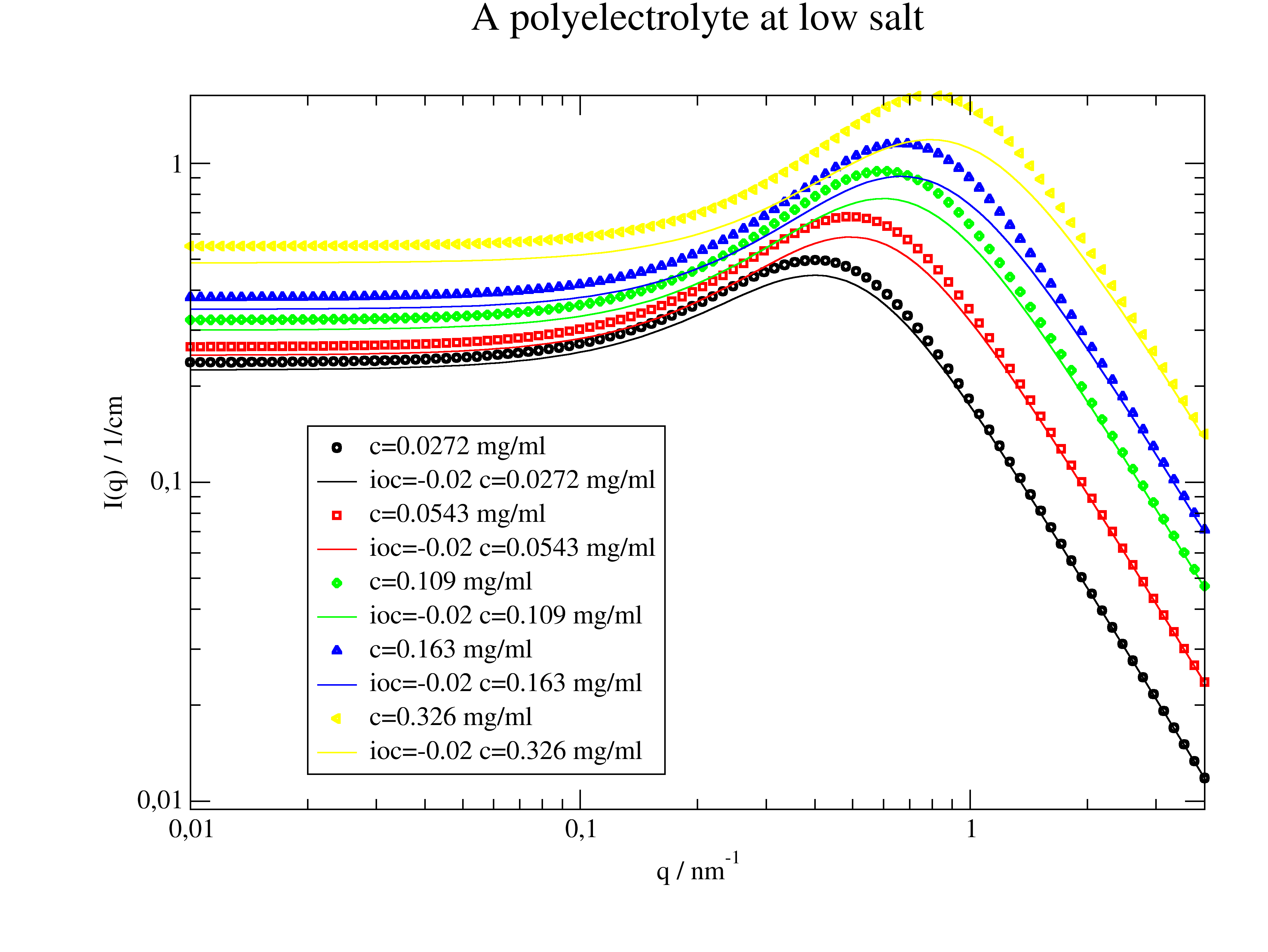
Monomer-monomer structure factor S(q) of a weak polyelectrolyte according to Borue and Erukhimovich [3]. |
|
Structure factor of a fractal cluster of particles following Teixeira (mass fractal). |
|
Freely jointed chain structure factor. |
ordered structures like crystals or lattices. Needs first to create a Lattice.
|
Radial structure factor S(q) in powder average of a crystal lattice with particle asymmetry, Debye-Waller factor, diffusive scattering and broadening due to domain size. |
|
3D structure factor S(q) in powder average of a crystal lattice with particle asymmetry, DebyeWaller factor, diffusive scattering and broadening due to domain size. |
|
3D Structure factor S(q) of an oriented crystal lattice including particle asymmetry, DebyeWaller factor, diffusive scattering, domain rotation and domain size. |
|
Radial averaged structure factor S(q) of an oriented crystal lattice calculated as orientedLatticeStructureFactor. |
|
Bragg peaks and diffuse scattering from lamellar structures. |
7.2. Hydrodynamics
|
Hydrodynamic function H(q) from hydrodynamic pair interaction of spheres in suspension. |
7.3. Pair Correlation
|
Radial distribution function g(r) from structure factor S(Q). |
7.4. Lattice
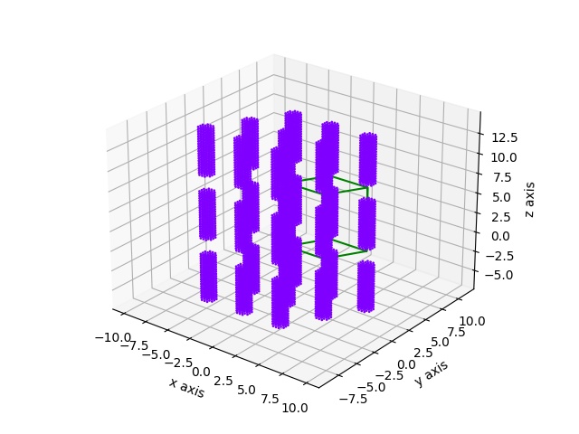
Lattices to describe atomic crystals or mesoscopic materials as ordered structures of spheres, ellipsoids, cylinders or planes in 3D (fcc, bcc, hcp, sc), 2D (hex, sq) and lamellar structures. For the later it is assumed that particles share the same normalised formfactor but allow particle specific scattering amplitude.
The small angle scattering or wide angle scattering (SAXS/WAXS) of a nano particle build from a lattice may be calculated by
cloudScattering()ororientedCloudScattering().The crystal structure factor of a lattice may be calculated by
latticeStructureFactor()ororientedLatticeStructureFactor()(see examples within these).To create your own lattice e.g. with a filled unit cell see the source code of one of the predefined lattices or latticeFromMDA.
Examples
|
|

|
A hollow sphere cut to a wedge.
import jscatter as js
import numpy as np
grid = js.lattice.scLattice(1/2.,2*8,b=[0])
grid.inSphere(6,b=1)
grid.inSphere(4,b=0)
grid.planeSide([1,1,1],b=0)
grid.planeSide([1,-1,-1],b=0)
fig = grid.show()

q=js.loglist(0.01,5,600)
ffe=js.ff.cloudScattering(q,grid.points,relError=0.02,rms=0.1)
p=js.grace()
p.plot(ffe)
# fig.savefig(js.examples.imagepath+'/grid_wedge.jpg')
A cube decorated with spheres.
import jscatter as js
import numpy as np
grid= js.lattice.scLattice(0.2,2*15,b=[0])
v1=np.r_[4,0,0]
v2=np.r_[0,4,0]
v3=np.r_[0,0,4]
grid.inParallelepiped(v1,v2,v3,b=1)
grid.inSphere(1,center=[0,0,0],b=2)
grid.inSphere(1,center=v1,b=3)
grid.inSphere(1,center=v2,b=4)
grid.inSphere(1,center=v3,b=5)
grid.inSphere(1,center=v1+v2,b=6)
grid.inSphere(1,center=v2+v3,b=7)
grid.inSphere(1,center=v3+v1,b=8)
grid.inSphere(1,center=v3+v2+v1,b=9)
fig = grid.show()

q=js.loglist(0.01,5,600)
ffe=js.ff.cloudScattering(q,grid.points,relError=0.02,rms=0.)
p=js.grace()
p.plot(ffe)
# fig.savefig(js.examples.imagepath+'/grid_cubewithspheres.jpg')
An explicit comparison of sc, bcc and fcc nanoparticles (takes a while )
The diffuse scattering appears as a consequence of thermal disorder described by random displacements from parameter rms=0.05 nm.
import jscatter as js
import numpy as np
q=js.loglist(0.01,35,1500)
q=np.r_[js.loglist(0.01,3,200),3:40:800j]
unitcelllength=1.5
N=8

scgrid= js.lattice.scLattice(unitcelllength,N)
sc=js.ff.cloudScattering(q,scgrid.points,relError=50,rms=0.05)
bccgrid= js.lattice.bccLattice(unitcelllength,N)
bcc=js.ff.cloudScattering(q,bccgrid.points,relError=50,rms=0.05)
fccgrid= js.lattice.fccLattice(unitcelllength,N)
fcc=js.ff.cloudScattering(q,fccgrid.points,relError=50,rms=0.05)

p=js.grace(1.5,1)
# smooth with Gaussian to include instrument resolution
p.plot(sc.X,js.formel.smooth(sc,10, window='gaussian'),legend='sc')
p.plot(bcc.X,js.formel.smooth(bcc,10, window='gaussian'),legend='bcc')
p.plot(fcc.X,js.formel.smooth(fcc,10, window='gaussian'),legend='fcc')

q=q=js.loglist(1,35,100)
p.plot(q,(1-np.exp(-q*q*0.05**2))/scgrid.shape[0],li=1,sy=0,le='sc diffusive')
p.plot(q,(1-np.exp(-q*q*0.05**2))/bccgrid.shape[0],li=2,sy=0,le='bcc diffusive')
p.plot(q,(1-np.exp(-q*q*0.05**2))/fccgrid.shape[0],li=3,sy=0,le='fcc diffusive')

p.title('Comparison sc, bcc, fcc lattice for a nano cube')
p.yaxis(scale='l',label='I(Q)')
p.xaxis(scale='l',label='Q / A\S-1')
p.legend(x=0.03,y=0.001,charsize=1.5)
p.text('cube formfactor',x=0.02,y=0.05,charsize=1.4)
p.text('Bragg peaks',x=4,y=0.05,charsize=1.4)
p.text('diffusive scattering',x=4,y=1e-6,charsize=1.4)
# p.save(js.examples.imagepath+'/cubicLatticeComparisonExplicit.jpg',size=(1.4,1),dpi=300)
Lattice creation
|
Create a rhombic lattice with specified unit cell atoms which can also represent lattices of mesoscopic particles. |
|
Create lattice as defined in CIF (Crystallographic Information Format) file or a pymatgen structure. |
|
Create lattice with a unit cell defined from MDAnalysis universe atomgroup. |
|
Lattice vectors from lattice constants. |
predefined 3D
|
Create a Bravais lattice. |
|
Simple Cubic lattice. |
|
Body centered cubic lattice. |
|
Face centered cubic lattice. |
|
Hexagonal lattice. |
|
Hexagonal closed packed lattice. |
|
Diamond cubic lattice with 8 atoms in unit cell. |
|
Honeycomb lattice e.g for graphene. |
|
Create a lattice with a random distribution of points. |
|
Create a lattice with a pseudo random distribution of points. |
predefined 2D
|
Simple 2D square lattice. |
|
Simple 2D hexagonal lattice. |
predefined 1D
|
1D lamellar lattice. |
general lattice methods :
X coordinates for b!=0 |
|
X coordinates |
|
Y coordinates for b!=0 |
|
Y coordinates |
|
Z coordinates for b!=0 |
|
Z coordinates |
|
X,Y,Z coordinates array Nx3 for b!=0 |
|
X,Y,Z coordinates array Nx3 |
|
Scattering length for points with b!=0 |
|
Scattering length all points |
|
Coordinates and scattering length as array for b!=0 |
|
Points with scattering length !=0 |
|
|
Set all points to given scattering length. |
|
Set b of all points (including points with b==0) according to selection. |
Returns type of the lattice |
|
|
Move all points by vector. |
Center of mass as center of geometry. |
|
Number of Atoms |
|
|
Show the lattice in matplotlib with scattering length color coded. |
|
Set lattice points scattering length according to a function. |
|
Prune lattice to reduced number of points (in place). |
|
Set scattering length for points on one side of a plane. |
|
Set scattering length for points in sphere. |
|
Set scattering length for points in ellipsoid. |
|
Set scattering length for points in parallelepiped. |
|
Set scattering length for points within a long cylinder. |
rhombic lattice methods :
Absolute positions of unit cell atoms. |
|
|
Reciprocal lattice of given size with peak scattering intensity. |
Get radial distribution of Bragg peaks with unit cell structure factor and multiplicity. |
|
|
Get scattering angle \(\theta=2arcsin(q_{hkl}\lambda/4\pi)\) in degrees. |
Rotate lattice by rotation matrix including reciprocal vectors (in place). |
|
|
Rotate plane points that plane is perpendicular to hkl direction. |
|
Rotate plane points around hkl direction. |
|
Rotate lattice that hkl direction is parallel to vector. |
|
Rotate lattice around hkl direction by angle or to align to vector. |
|
Get vector corresponding to hkl direction. |
random lattice methods
|
Add points to pseudorandom lattice. |
- class jscatter.sf.lattice[source]
Bases:
objectCreate an arbitrary lattice.
Please use one of the subclasses below for creation.
pseudorandom, rhombicLattice, bravaisLattice scLattice, bccLattice, fccLattice, diamondLattice, hexLattice, hcpLattice, sqLattice, hexLattice, lamLattice
This base class defines methods valid for all subclasses.
- isLattice = True
- property dimension
- property X
X coordinates for b!=0
- property Xall
X coordinates
- property Y
Y coordinates for b!=0
- property Yall
Y coordinates
- property Z
Z coordinates for b!=0
- property Zall
Z coordinates
- property XYZ
X,Y,Z coordinates array Nx3 for b!=0
- property XYZall
X,Y,Z coordinates array Nx3
- property b
Scattering length for points with b!=0
- property ball
Scattering length all points
- property shape
Shape for points with b!=0
- property shapeall
Shape for points with b!=0
- property type
Returns type of the lattice
- property array
Coordinates and scattering length as array for b!=0
- set_b(b)[source]
Set all points to given scattering length.
- Parameters:
- bfloat or array length points
- set_bsel(b, select)[source]
Set b of all points (including points with b==0) according to selection.
To access all points us the properties grid.??all which contains all coordinates and b.
- Parameters:
- bfloat or array length _points
Scattering length
- selectbool array
Selection array of len(grid.ball)
Examples
grid.set_ball(1, grid.Xall > 0)
- property points
Points with scattering length !=0
grid._points contains all Nx[x,y,z,b]
- property nonzerob
Mask of nonzero b.
- prune(select=None)[source]
Prune lattice to reduced number of points (in place).
- Parameters:
- selectbool array xN or function
A bool array of length grid points to keep only points that are true or a bool function that is evaluated for each [x,y,z,b] evaluating to True. By default all pounts with b=0 are removed.
Examples
grid.prune(grid.ball>0)  # bool array
grid.prune(lambda a:a[3]>0)  # function
- filter(funktion)[source]
Set lattice points scattering length according to a function.
All points in the lattice are changed for which funktion returns value !=0 (tolerance 1e-12).
- Parameters:
- funktionfunction returning float
Function to set lattice points scattering length. The function is applied with each i point coordinates (array) as input as .points[i,:3]. The return value is the corresponding scattering length.
Examples
# To select points inside of a sphere with radius 5 around [1,1,1]:
from numpy import linalg as la
sc=js.sf.scLattice(0.9,10)
sc.set_b(0)
sc.filter(lambda xyz: 1 if la.norm(xyz-np.r_[1,1,1])<5 else 0)

# sphere with  increase from center
from numpy import linalg as la
sc=js.sf.scLattice(0.9,10)
sc.set_b(0)
sc.filter(lambda xyz: 2*(la.norm(xyz)) if la.norm(xyz)<5 else 0)
fig=sc.show()
- move(vector)[source]
Move all points by vector.
- Parameters:
- vectorlist of 3 float or array
Vector to shift the points.
- inParallelepiped(v1, v2, v3, corner=None, b=1, invert=False)[source]
Set scattering length for points in parallelepiped.
- Parameters:
- corner3x float
Corner of parallelepiped
- v1,v2,v3each 3x float
Vectors from origin to 3 corners that define the parallelepiped.
- b: float
Scattering length for selected points.
- invertbool
Invert selection
Examples
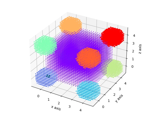
import jscatter as js
sc=js.sf.scLattice(0.2,10,b=[0])
sc.inParallelepiped([1,0,0],[0,1,0],[0,0,1],[0,0,0],1)
sc.show()
sc=js.sf.scLattice(0.1,30,b=[0])
sc.inParallelepiped([1,1,0],[0,1,1],[1,0,1],[-1,-1,-1],2)
sc.show()
- planeSide(vector, center=None, b=1, invert=False)[source]
Set scattering length for points on one side of a plane.
- Parameters:
- center3x float, default [0,0,0]
Point in plane.
- vectorlist 3x float
Vector perpendicular to plane.
- b: float
Scattering length for selected points.
- invertbool
False choose points at origin side. True other side.
Examples
sc=js.sf.scLattice(1,10,b=[0])
sc.planeSide([1,1,1],[3,3,3],1)
sc.show()
sc.planeSide([-1,-1,0],3)
sc.show()
- inSphere(R, center=None, b=1, invert=False)[source]
Set scattering length for points in sphere.
- Parameters:
- center3 x float, default [0,0,0]
Center of the sphere.
- R: float
Radius of sphere around origin.
- b: float
Scattering length for selected points.
- invertbool
True to invert selection.
Examples
import jscatter as js
sc=js.sf.scLattice(1,15,b=[0])
sc.inSphere(6,[2,2,2],b=1)
sc.show()
sc.inSphere(6,[-2,-2,-2],b=2)
sc.show()

sc=js.sf.scLattice(0.8,20,b=[0])
sc.inSphere(3,[2,2,2],b=1)
sc.inSphere(3,[-2,-2,-2],b=1)
sc.show()

sc=js.sf.scLattice(0.8,20,b=[0])
sc.inSphere(3,[2,2,2],b=1)
sc.inSphere(4,[0,0,0],b=2)
sc.show()
- inEllipsoid(abc, rotation=None, center=None, b=1, invert=False)[source]
Set scattering length for points in ellipsoid.
- Parameters:
- abc: [float,float,float]
Principal semi axes length of the ellipsoid.
- rotationscipy.spatial.transform.Rotation object
Rotation describing the rotation semi axes rotation from the cartesian axes. e.g. scipy.spatial.transform.Rotation.from_rotvec([np.pi/4, 0, 0])
- center3 x float, default [0,0,0]
Center of the sphere.
- b: float
Scattering length for selected points.
- invertbool
True to invert selection.
Examples
import jscatter as js
from scipy.spatial.transform import Rotation as R
sc=js.sf.scLattice(0.5,30,b=[0])
sc.inEllipsoid(abc=[3,1,12],b=1)
sc.show()
sc.inEllipsoid(abc=[3,1,12],rotation=R.from_euler('X',45,degrees=True),b=2)
sc.show()
sc.inEllipsoid(abc=[3,1,12],rotation=R.from_euler('XY',[45,90],degrees=True),b=3)
sc.show()
- inCylinder(v, R, a=None, length=0, b=1, invert=False)[source]
Set scattering length for points within a long cylinder.
- Parameters:
- a3 x float, default [0,0,0]
Edge point on cylinder axis.
- Rfloat
Radius of cylinder.
- v3 x float
Normal vector along cylinder axis.
- length
Length along cylinder axis.
<0 negative direction
>0 positive direction
=0 infinite both directions
np.inf positive direction, infinite length
np.ninf negative direction, infinite length
- b: float
Scattering length for selected points.
- invertbool
True to invert selection.
Examples
import jscatter as js
import numpy as np
sc=js.sf.scLattice(0.5,30,b=[0])
sc.inCylinder(v=[1,1,1],a=[5,0,5],R=3)
sc.inCylinder(v=[1,-1,1],a=[0,5,0],R=2)
sc.inCylinder(v=[1,0,0],a=[0,-5,-10],length =10,R=2)
sc.inCylinder(v=[0,1,0],a=[5,0,-10],length =10,R=2)
sc.inCylinder(v=[1,0,0],a=[-10,-5,10],length =10,R=2,b=2)
sc.inCylinder(v=[0,1,0],a=[-5,0,10],length =-10,R=2,b=2)
sc.inCylinder(v=[1,0,0],a=[0,5,-10],length =np.NINF,R=2)
sc.show()
- alongLine(v, R, a=None, length=0, b=1, invert=False)
Set scattering length for points within a long cylinder.
- Parameters:
- a3 x float, default [0,0,0]
Edge point on cylinder axis.
- Rfloat
Radius of cylinder.
- v3 x float
Normal vector along cylinder axis.
- length
Length along cylinder axis.
<0 negative direction
>0 positive direction
=0 infinite both directions
np.inf positive direction, infinite length
np.ninf negative direction, infinite length
- b: float
Scattering length for selected points.
- invertbool
True to invert selection.
Examples
import jscatter as js
import numpy as np
sc=js.sf.scLattice(0.5,30,b=[0])
sc.inCylinder(v=[1,1,1],a=[5,0,5],R=3)
sc.inCylinder(v=[1,-1,1],a=[0,5,0],R=2)
sc.inCylinder(v=[1,0,0],a=[0,-5,-10],length =10,R=2)
sc.inCylinder(v=[0,1,0],a=[5,0,-10],length =10,R=2)
sc.inCylinder(v=[1,0,0],a=[-10,-5,10],length =10,R=2,b=2)
sc.inCylinder(v=[0,1,0],a=[-5,0,10],length =-10,R=2,b=2)
sc.inCylinder(v=[1,0,0],a=[0,5,-10],length =np.NINF,R=2)
sc.show()
- property lastSelection
Give last selection from filter, inSphere, inCylinder, inEllipsoid, planeSide, inParallelepiped.
- show(R=None, cmap='rainbow', fig=None, ax=None, atomsize=1)[source]
Show the lattice in matplotlib with scattering length color coded.
- Parameters:
- Rfloat,None
Radius around origin to show.
- cmapcolormap
Colormap. E.g. ‘rainbow’, ‘winter’,’autumn’,’gray’ to color atoms according to their scattering length b. Use js.mpl.showColors() for all possibilities.
- figmatplotlib Figure
Figure to plot in. If None a new figure is created.
- axAxes
If given this axes is used for plotting.
- atomsizefloat
Sphere size of the atoms. Unfortunately matplotlib does not scale the point size when zooming.
- Returns:
- fig handle
Notes
If the three dimensional overlap is wrong this is due to matplotlib. matplotlib is not a real 3D graphic program.
- class jscatter.sf.rhombicLattice(latticeVectors, size, unitCellAtoms=None, b=None)[source]
Bases:
latticeCreate a rhombic lattice with specified unit cell atoms which can also represent lattices of mesoscopic particles.
Allows to create 1D, 2D or 3D latices by using 1, 2 or 3 latticeVectors. This can generate classical Bravais lattices but the unit cell atom may also build a coarse grained complex particle like a cylinder or ellipsoid. In
latticeStructureFactor()the particle formfactor amplitude is taken into account.- Parameters:
- latticeVectorslist of array 3x1
Lattice vectors defining the translation of the unit cell along its principal axes.
- size :list of integer
A list of integers describing the size in direction of the respective latticeVectors. Size is symmetric around zero in interval [-i,..,i] with length 2i+1.
- unitCellAtomslist of 3x1 array, None=[0,0,0]
Position vectors vi of atoms in the unit cell in relative units of the lattice vectors [0<x<1]. For 2D and 1D the unit cell atoms vectors are len(vi)=2 and len(vi)=1.
- blist of float
Corresponding scattering length of atoms in the unit cell.
- Returns:
- lattice object
.array : grid points as numpy array
.unitCellVolume : V = a1*a2 x a3 with latticeVectors a1, a2, a3; if existing.
.dim : dimensionality
.unitCellAtoms : Unit cell atoms in relative coordinates
.unitCellAtoms_b : Scattering length of specific unit cell atoms
Examples
A diatomic base
import jscatter as js
grid=js.sf.rhombicLattice(latticeVectors=[[1,0,0],[0,1,0],[0,0,1]],
                           size=[3,3,3],
                           unitCellAtoms=[[-0.1,-0.1,-0.1],[0.1,0.1,0.1]],
                           b=[1,2])
grid.show(1.5)
A cylinder in a hexagonal lattice
import jscatter as js
import numpy as np

# create lattice vectors in a simple way
hex = js.sf.hexLattice(4,8,1)

# create cylinder with atoms in much shorter distance than hex lattice
cylinder = js.sf.scLattice(0.3,[6,6,13])
cylinder.move([0,0,3])
cylinder.inCylinder(v=[0,0,1], R=0.8, a=[0,0,0.5], length=6, b=0, invert=True)

# Convert the cylinder points coordinates to
# fractional unit cell coordinates of the hexagonal lattice
mat = np.linalg.inv(hex.latticeVectors).T
cellAtoms = mat @ cylinder.XYZ.T

grid=js.sf.rhombicLattice(latticeVectors=hex.latticeVectors,
                           size=[1,1,1],
                           unitCellAtoms=cellAtoms.T,
                           b=cylinder.b)
fig = grid.show()
# fig.savefig(js.examples.imagepath+'/grid_hexlyotropic.jpg')
- isRhombic = True
- property unitCellAtomPositions
Absolute positions of unit cell atoms.
- getReciprocalLattice(size=2, threshold=0.001)[source]
Reciprocal lattice of given size with peak scattering intensity.
- Parameters:
- size3x int or int, default 2
Number of reciprocal lattice points in each direction (+- direction).
- thresholdfloat
Threshold for selection rule as select if (f2_hkl > max(f2_hkl)*threshold)
- Returns:
- Array [N x 7] with
reciprocal lattice vectors [:,:3] corresponding structure factor fhkl**2>0 [:, 3] corresponding indices hkl [:,4:]
Notes
The threshold for selection rules allows to exclude forbidden peaks but include these for unit cells with not equal scattering length as in these cases the selection rule not applies to full extend. This is prefered over a explicit list of selection rules.
- getRadialReciprocalLattice(size)[source]
Get radial distribution of Bragg peaks with unit cell structure factor and multiplicity.
To get real Bragg peak intensities the dimension in lattice directions has to be included (+ Debye-Waller factor and diffusive scattering). Use latticeStructureFactor to include these effects.
- Parameters:
- sizeint
Size of the lattice as maximum included Miller indices.
- Returns:
- list of [unique q values, structure factor fhkl(q)**2, multiplicity mhkl(q), hkl indices]
Notes
The list contains distinct reflections. If multiplicities are different than expected, e.g. 18 for hex2D the reason is that peaks are degenerate as hk {35} and {70} result in the same Q adding up the multiplicity 18=6+12 . In the radial reciprocal lattice these cannot be separated.
- getScatteringAngle(wavelength=None, size=13)[source]
Get scattering angle \(\theta=2arcsin(q_{hkl}\lambda/4\pi)\) in degrees.
- Parameters:
- wavelengthfloat, 0.15406
Wavelength \(\lambda\) in unit nm, default is Cu K-alpha 0.15406 nm.
- sizeint
Maximum size of reciprocal lattice.
- Returns:
- array in degrees
- vectorhkl(hkl)[source]
Get vector corresponding to hkl direction.
- Parameters:
- hkl3x float
Miller indices
- Returns:
- array 3x float
- rotatePlane2hkl(plane, hkl, basis=None)[source]
Rotate plane points that plane is perpendicular to hkl direction.
- Parameters:
- planearray Nx3
3D points of plane to rotate. If None the rotation matrix is returned.
- hkllist of int, float
Miller indices as [1,1,1] indicating the lattice direction where to rotate to.
- basisarray min 3x3, default=None
3 basis points spanning the plane to define rotation. e.g.[[0,0,0],[1,0,0],[0,1,0]] for xy plane. If None the first points of the plane are used instead.
- Returns:
- rotated plane points array 3xN
- or rotation matrix 3x3
Notes
The rotation matrix may be used to rotate the plane to the desired direction.
R = grid.rotatePlane2hkl(None,[1,1,1],[[0,0,0],[1,0,0],[0,1,0]] )
newplanepoints = np.einsum('ij,kj->ki', R, planepoints)
or the transposed R can be used to rotate the lattice.
R = grid.rotatePlane2hkl(None,[1,1,1],[[0,0,0],[1,0,0],[0,1,0]] )
grid.rotatebyMatrix(R.T)
Examples
import jscatter as js
import numpy as np
R=8
N=10
qxy=np.mgrid[-R:R:N*1j, -R:R:N*1j].reshape(2,-1).T
qxyz=np.c_[qxy,np.zeros(N**2)]
fccgrid = js.lattice.fccLattice(2.1, 2)
xyz=fccgrid.rotatePlane2hkl(qxyz,[1,1,1])

p=js.mpl.scatter3d(xyz[:,0],xyz[:,1],xyz[:,2])
p.axes[0].scatter(fccgrid.X,fccgrid.Y,fccgrid.Z)
- rotatePlaneAroundhkl(plane, hkl, angle)[source]
Rotate plane points around hkl direction.
- Parameters:
- planearray Nx3, None
3D points of plane. If None the rotation matrix is returned.
- hkllist of int, float
Miller indices as [1,1,1] indicating the lattice direction to rotate around.
- anglefloat
Angle in rad
- Returns:
- plane points array 3xN
- or rotation matrix
Notes
The rotation matrix may be used to rotate the plane to the desired direction.
R = grid.rotatePlaneAroundhkl(None,[1,1,1],1.234)
newplanepoints = np.einsum('ij,kj->ki', R, planepoints)
or the transposed R can be used to rotate the lattice.
grid.rotatebyMatrix(R.T)
Examples
import jscatter as js
import numpy as np
R=8
N=10
qxy=np.mgrid[-R:R:N*1j, -R:R:N*1j].reshape(2,-1).T
qxyz=np.c_[qxy,np.zeros(N**2)]
fccgrid = js.lattice.fccLattice(2.1, 1)
xyz=fccgrid.rotatePlane2hkl(qxyz,[1,1,1])
xyz2=fccgrid.rotatePlaneAroundhkl(xyz,[1,1,1],np.deg2rad(30))
p=js.mpl.scatter3d(xyz[:,0],xyz[:,1],xyz[:,2])
p.axes[0].scatter(xyz2[:,0],xyz2[:,1],xyz2[:,2])
p.axes[0].scatter(fccgrid.X,fccgrid.Y,fccgrid.Z)
- rotatehkl2Vector(hkl, vector)[source]
Rotate lattice that hkl direction is parallel to vector.
Includes rotation of latticeVectors.
- Parameters:
- hkl3x float
Direction given as Miller indices.
- vector3x float
Direction to align to.
Examples
import jscatter as js
import numpy as np
R=8
N=10
qxy=np.mgrid[-R:R:N*1j, -R:R:N*1j].reshape(2,-1).T
qxyz=np.c_[qxy,np.zeros(N**2)]

fccgrid = js.lattice.fccLattice(2.1, 1)
p=js.mpl.scatter3d(fccgrid.X,fccgrid.Y,fccgrid.Z)

fccgrid.rotatehkl2Vector([1,1,1],[1,0,0])
p.axes[0].scatter(fccgrid.X,fccgrid.Y,fccgrid.Z)

fccgrid.rotateAroundhkl([1,1,1],np.deg2rad(30))
p.axes[0].scatter(fccgrid.X,fccgrid.Y,fccgrid.Z)
- rotateAroundhkl(hkl, angle=None, vector=None, hkl2=None)[source]
Rotate lattice around hkl direction by angle or to align to vector.
Uses angle or aligns hkl2 to vector. Includes rotation of latticeVectors.
- Parameters:
- hkl3x float
Direction given as Miller indices.
- anglefloat
Rotation angle in rad.
- vector3x float
Vector to align hkl2 to. Overrides angle. Should not be parallel to hkl direction.
- hkl23x float
Direction to align along vector. Overrides angle. Should not be parallel to hkl direction.
Examples
import jscatter as js
import numpy as np
R=8
N=10
qxy=np.mgrid[-R:R:N*1j, -R:R:N*1j].reshape(2,-1).T
qxyz=np.c_[qxy,np.zeros(N**2)]
fccgrid = js.lattice.fccLattice(2.1, 1)
fig=js.mpl.figure( )
# create subplot to define geometry
fig.add_subplot(2,2,1,projection='3d')
fccgrid.show(fig=fig,ax=1)
fccgrid.rotatehkl2Vector([1,1,1],[1,0,0])
fccgrid.show(fig=fig,ax=2)
fccgrid.rotateAroundhkl([1,1,1],np.deg2rad(30))
fccgrid.show(fig=fig,ax=3)
fccgrid.rotateAroundhkl([1,1,1],[1,0,0],[1,0,0])
fccgrid.show(fig=fig,ax=4)
Fluid like and crystal like structure factors (sf) and directly related functions for scattering related to interaction potentials between particles.
Fluid like include hard core SF or charged sphere sf and more. For RMSA an improved algorithm is used based on the original idea (see Notes in RMSA).
For lattices of ordered mesoscopic materials (see Lattice) the analytic sf can be calculated in powder average or as oriented lattice with domain rotation.
Additionally, the structure factor of atomic lattices can be calculated using atomic scattering length. Using coordinates from CIF (Crystallographic Information Format) file allow calculation of atomic crystal lattices.
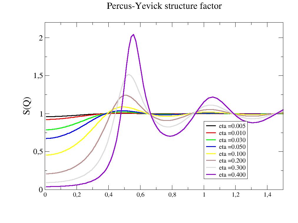
- jscatter.sf.PercusYevick(q, R, molarity=None, eta=None)[source]
The Percus-Yevick structure factor of a hard sphere in 3D.
- Parameters:
- qarray; N dim
scattering vector; units 1/(R[unit])
- Rfloat
Radius of the object
- etafloat
volume fraction as eta=4/3*pi*R**3*n with number density n in units or R
- molarityfloat
number density in mol/l and defines q and R units to 1/nm and nm to be correct preferred over eta if both given
- Returns:
- dataArray
structure factor for given q
Notes
Structure factor for the potential in 3D
\[\begin{split}\begin{align} U(r) & = \infty \ & r<=R \\ & = 0 \ & r>R \end{align}\end{split}\]The Problem is given in [1]; the solution in [2] and the best description of the solution is in [3].
References
[1]Percus and G. J. Yevick, Phys. Rev. 110, 1 (1958).
[2]Wertheim, Phys. Rev. Lett. 10, 321 (1963).
[3]Kinning and E. L. Thomas, Macromolecules 17, 1712 (1984).
Examples
import jscatter as js
R = 6
phi = 0.05
depth = 15
q = js.loglist(0.01, 2, 200)
p = js.grace(1,1)
for eta in [0.005,0.01,0.03,0.05,0.1,0.2,0.3,0.4]:
    py = js.sf.PercusYevick(q, R, eta=eta)
    p.plot(py, symbol=0, line=[1, 3, -1], legend=f'eta ={eta:.3f}')
p.yaxis(min=0.0, max=2.2, label='S(Q)', charsize=1.5)
p.legend(x=1, y=0.9)
p.xaxis(min=0, max=1.5)
p.title('3D Percus-Yevick structure factor')
#p.save(js.examples.imagepath+'/PercusYevick.jpg')
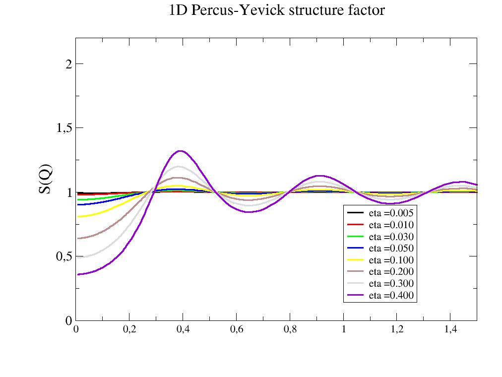
- jscatter.sf.PercusYevick1D(q, R=1, eta=0.1)[source]
The PercusYevick structure factor of a hard sphere in 1D.
Structure factor for the potential U(r)= (inf for 0<r<R) and (0 for R<r).
- Parameters:
- qarray; N dim
scattering vector; units 1/(R[unit])
- Rfloat
Radius of the object in nm.
- etafloat
Packing fraction as eta=2*R*n with number density n.
- Returns:
- dataArray
[q,structure factor]
Notes
Structure factor for the potential in 1D
\[\begin{split}\begin{align} U(r) & = \infty \ & r<=R \\ & = 0 \ & r>R \end{align}\end{split}\]References
[1]Exact solution of the Percus-Yevick equation for a hard-core fluid in odd dimensions Leutheusser E Physica A 1984 vol: 127 (3) pp: 667-676
[2]On the equivalence of the Ornstein–Zernike relation and Baxter’s relations for a one-dimensional simple fluid Chen M Journal of Mathematical Physics 1975 vol: 16 (5) pp: 1150
Examples
import jscatter as js
R = 6
phi = 0.05
depth = 15
q = js.loglist(0.01, 2, 200)
p = js.grace(1,1)
for eta in [0.005,0.01,0.03,0.05,0.1,0.2,0.3,0.4]:
    py = js.sf.PercusYevick1D(q, R, eta=eta)
    p.plot(py, symbol=0, line=[1, 3, -1], legend=f'eta ={eta:.3f}')
p.yaxis(min=0.0, max=2.2, label='S(Q)', charsize=1.5)
p.legend(x=1, y=0.9)
p.xaxis(min=0, max=1.5)
p.title('1D Percus-Yevick structure factor')
#p.save(js.examples.imagepath+'/PercusYevick1D.jpg')
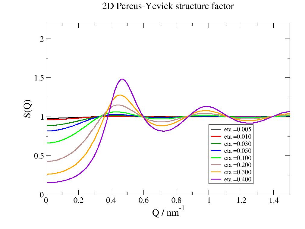
- jscatter.sf.PercusYevick2D(q, R=1, eta=0.1, a=None)[source]
The PercusYevick structure factor of a hard sphere in 2D.
- Parameters:
- qarray; N dim
Scattering vector; units 1/(R[unit])
- Rfloat, default 1
Radius of the object
- etafloat, default 0.1
Packing fraction as eta=pi*R**2*n with number density n maximum hexagonal closed packed \(eta= (\pi R^2)/(3/2 3^{1/2}a^2)\) \(R_{max}=a 3^{1/2}/2\) with max packing of 0.9069.
- afloat, default None
Calculate eta from hexagonal lattice constant a as \(eta=\frac{2\pi R^2}{3\sqrt{3}a^2}\). This keeps the average distance of the sphere constant.
- Returns:
- dataArray
Notes
Structure factor for the potential in 2D
\[\begin{split}\begin{align} U(r) & = \infty \ & r<=R \\ & = 0 \ & r>R \end{align}\end{split}\]References
[1]Free-energy model for the inhomogeneous hard-sphere fluid in D dimensions: Structure factors for the hard-disk (D=2) mixtures in simple explicit form Yaakov Rosenfeld Phys. Rev. A 42, 5978
Examples
import jscatter as js
R = 6
phi = 0.05
depth = 15
q = js.loglist(0.01, 2, 200)
p = js.grace(1,1)
for eta in [0.005,0.01,0.03,0.05,0.1,0.2,0.3,0.4]:
    py = js.sf.PercusYevick2D(q, R, eta=eta)
    p.plot(py, symbol=0, line=[1, 3, -1], legend=f'eta ={eta:.3f}')
p.yaxis(min=0.0, max=2.2, label='S(Q)', charsize=1.5)
p.legend(x=1, y=0.9)
p.xaxis(label='Q / nm\S-1',min=0, max=1.5, charsize=1.5)
p.title('2D Percus-Yevick structure factor')
# p.save(js.examples.imagepath+'/PercusYevick2D.jpg')
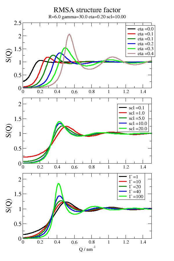
- jscatter.sf.RMSA(q, R, scl, gamma, molarity=None, eta=None, useHP=False)[source]
Structure factor for a screened coulomb interaction (single Yukawa) in rescaled mean spherical approximation (RMSA).
Structure factor according to Hayter-Penfold [1] [2] . Consider a scattering system consisting of macro ions, counter ions and solvent. Here an improved algorithm [3] is used based on the original idea described in [1] (see Notes).
- Parameters:
- qarray; N dim
Scattering vector in units 1/nm.
- Rfloat
Radius of the object \(\sigma\) in units nm.
- molarityfloat
Number density n in units mol/l. Overrides eta, if both given.
- sclfloat>0
Screening length, Debye length or Debye–Hückel screening length \(\lambda=1/\kappa\) in units nm. Negative values evaluate to scl=0.
- gammafloat
Contact potential \(\gamma\) in units kT.
\(\gamma=Z_m/(\pi \epsilon \epsilon_0 R (2+\kappa R))\)
\(Z_m = Z^*\) effective surface charge
\(\epsilon_0,\epsilon\) free permittivity and dielectric constant
\(\kappa=1/\lambda\) inverse screening length
- etafloat
Volume fraction as \(eta=\Phi=4/3piR^3n\) with number density n.
- useHPbool, default False
To use the original Hayter/Penfold algorithm. This gives wrong results for some parameter conditions. It should ONLY be used for testing. See example examples/test_newRMSAAlgorithm.py for a direct comparison.
- Returns:
- dataArray
.volumeFraction = eta
.rescaledVolumeFraction
.screeningLength
.gamma=gamma
.contactpotential
.S0 structure factor at q=0
.scalingfactor factor for rescaling to get g+1=0; if =1 nothing was scaled and it is MSA
Notes
The repulsive potential between two identical spherical macroions of diameter \(\sigma\) is (DLVO model) in dimensionless form
\[\begin{split}\frac{U(x)}{k_BT} &= \gamma \frac{e^{-kx}}{x} \; &for \; x>1 \\ &= \infty &for \; x<1\end{split}\]\(x = r/\sigma, k=\kappa\sigma, K=Q\sigma\) dimesionless parameters
\(k_BT\) thermal energy
\(\gamma e^{-k} = \frac{\pi \epsilon_0 \epsilon \sigma }{k_BT} \psi^2_0\) contact potential in kT units
Inverse screening length \(\kappa\) with \(\kappa^2=4\pi \lambda_B \sum_i n_j z_j\)
with Bjerrum length \(\lambda_B = \frac{e^2}{4\pi \varepsilon_0 \varepsilon_r \ k_{B} T}\) using \(e\) elementary charge, \(\varepsilon_r\) relative dielectric constant of the medium, \(\varepsilon_0\) is the vacuum permittivity, \(n_i\) number density of ion i with charge z [unit e].
For water at room temperature \(T \approx 293 K\) \(\varepsilon_r \approx 80\), so that \(\lambda_B \approx 0.71 nm\) and \(\lambda[nm] = \frac{0.304}{I[M]}\) .
From [1]:
This potential is valid for colloid systems provided k < 6. There is no theoretical restriction on k in what follows, however, and for general studies of one component plasmas any value may be used.
In the limit \(\gamma \rightarrow 0\) or \(k\rightarrow\infty\) the Percus-Yevick hard sphere is reached.
Why is is named rescaled MSA: From [1]:
Note that in general, however, the MSA fails at low density; letting \(n\rightarrow0\) yields \(g(x)\rightarrow 1-lU(x)/kT\) for x> 1. Since U(x) is generally larger than thermal energies for small interparticle separations, g(x) will generally be negative (and hence unphysical) near the particle at very low densities. This does not present a problem for many colloid studies of current interest, where volume fractions are generally greater than 1%.
To solve this the radius is rescaled to get \(g(\sigma +)=0\) according to [2]:
…by increasing the particle diameter from its physical value a to an effective hard core value a’, while maintaining the Coulomb coupling constant. …
If \(g(\sigma +)>=0\) no rescaling is done.
Improved algorithm (see [3] fig. 6)
The Python code is deduced from the original Hayter-Penfold Fortran code (1981, ILL Grenoble). This is also used in other common SAS programs as SASfit or SASview (translated to C). The original algorithm determines the root of a quartic F(w1,w2,w3,w4) by an estimate (named PW estimate), refining it by a Newton algorithm. As the PW estimate is sometimes not good enough this results in an arbitrary root of the quartic in the Newton algorithm. The solution therefore jumps between different possibilities by small changes of the parameters. We use here the original idea from [1] to calculate G(r<0) for all four roots of F(w1,w2,w3,w4) and use the physical solution with G(r<R)=0. See examples/test_newRMSAAlgorithm.py for a direct comparison or [3] fig. 6.
Validity
The calculation of charge at the surface or screening length from a solute ion concentration is explicitly dedicate to the user. The Debye-Hückel theory for a macro ion in screened solution is a far field theory as a linearization of the Poisson-Boltzmann (PB) theory and from limited validity (far field or low charge -> linearization). Things like reverting charge layer, ion condensation at the surface, pH changes at the surface or other things might appear. Before calculating please take these things into account. Close to the surface the PB has to be solved. The DH theory can still be used if the charge is thus an effective charge named Z*, which might be different from the real surface charge. See Ref [4] for details.
Error Messages
   -1: 'NEWTON ITERATION NON-CONVERGENT IN _sqcoef',
   -2: 'NEWTON ITERATION NON-CONVERGENT IN _sqfun',
   -3: 'CANNOT RESCALE TO G(1+) > 0.',
   -4: 'no physical root with G(r<1) < 0.1 in _sqfun found'}

If errors appear the parameters are out of range (e.g a larger R leading to unreasonable volume fraction.)
To catch this during fitting limmit the respective parameters (eta<0.5) or use  (try: except ValueError).
References
[2]J.-P. Hansen and J. B. Hayter, Mol. Phys. 46, 651 (2006).
[3] (1,2,3)Jscatter, a program for evaluation and analysis of experimental data R.Biehl, PLOS ONE, 14(6), e0218789, 2019, https://doi.org/10.1371/journal.pone.0218789
[4]Belloni, J. Phys. Condens. Matter 12, R549 (2000).
Examples
Effect of volume fraction, surface potential and screening length onto RMSA structure factor
import jscatter as js
R = 6
eta0 = 0.2
gamma0 = 30 # surface potential
scl0 = 10
q = js.loglist(0.01, 5, 200)
p = js.grace(1,1.5)
p.multi(3,1)
for eta in [0.01,0.05,0.1,0.2,0.3,0.4]:
    rmsa = js.sf.RMSA(q, R, scl=scl0, gamma=gamma0, eta=eta)
    p[0].plot(rmsa, symbol=0, line=[1, 3, -1], legend=f'eta ={eta:.1f}')
for scl in [0.1,1,5,10,20]:
    rmsa = js.sf.RMSA(q, R, scl=scl, gamma=gamma0, eta=eta0)
    p[1].plot(rmsa, symbol=0, line=[1, 3, -1], legend=f'scl ={scl:.1f}')
for gamma in [1,10,20,40,100]:
    rmsa = js.sf.RMSA(q, R, scl=scl0, gamma=gamma, eta=eta0)
    p[2].plot(rmsa, symbol=0, line=[1, 3, -1], legend=r'\xG\f{} =$gamma')
p[0].yaxis(min=0.0, max=2.5, label='S(Q)', charsize=1.5)
p[0].legend(x=1.2, y=2.4)
p[0].xaxis(min=0, max=1.5,label='')
p[1].yaxis(min=0.0, max=2.2, label='S(Q)', charsize=1.5)
p[1].legend(x=1.1, y=2.)
p[1].xaxis(min=0, max=1.5, label=r'')
p[2].yaxis(min=0.0, max=2.2, label='S(Q)', charsize=1.5)
p[2].legend(x=1.1, y=2.2)
p[2].xaxis(min=0, max=1.5, label=r'Q / nm\S-1')
p[0].title('RMSA structure factor')
p[0].subtitle(f'R={R:.1f} gamma={gamma0:.1f} eta={eta0:.2f} scl={scl0:.2f}')
#p.save(js.examples.imagepath+'/rmsa.jpg',size=[600,900])
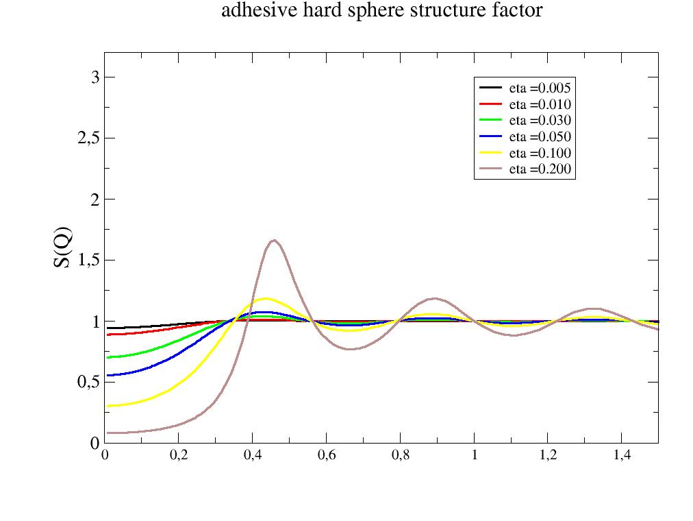
- jscatter.sf.adhesiveHardSphere(q, R, tau, delta, molarity=None, eta=None)[source]
Structure factor of a adhesive hard sphere potential (a square well potential)
- Parameters:
- qarray; N dim
Scattering vector; units 1/(R[unit])
- Rfloat
Radius of the hard core
- etafloat
Volume fraction of the hard core particles.
- molarityfloat
Number density in mol/l and defines q and R units to 1/nm and nm to be correct Preferred over eta if both given.
- taufloat
Stickiness \(\tau\)
- deltafloat
Width of the square well \(\delta\)
Notes
The potential U(d) for a distance d between particles with radius R is defined as
\[\begin{split}U(d) &= \infty & & d<2R \\ &= -depth=ln(\frac{12 \tau\delta}{2R+\delta})& \quad &2R<d<2R+\delta \\ &= 0 & & d>2R+\delta\end{split}\]References
[1]Regnaut and J. C. Ravey, J. Chem. Phys. 91, 1211 (1989).
[2]Regnaut and J. C. Ravey, J. Chem. Phys. 92 (5) (1990), 3250 Erratum
Examples
import jscatter as js
R = 6
phi = 0.05
depth = 15
q = js.loglist(0.01, 2, 200)
p = js.grace(1,1)
for eta in [0.005,0.01,0.03,0.05,0.1,0.2]:
    shs = js.sf.adhesiveHardSphere(q, R, 1, 3, eta=eta)
    p.plot(shs, symbol=0, line=[1, 3, -1], legend=f'eta ={eta:.3f}')
p.yaxis(min=0.0, max=3.2, label='S(Q)', charsize=1.5)
p.legend(x=1, y=3)
p.xaxis(min=0, max=1.5)
p.title('adhesive hard sphere structure factor')
#p.save(js.examples.imagepath+'/adhesiveHardSphere.jpg')
- class jscatter.sf.bccLattice(abc, size, b=None)[source]
Bases:
rhombicLatticeBody centered cubic lattice.
See rhombicLattice for methods.
- Parameters:
- abcfloat
Lattice constant of unit cell.
- size3x integer, integer
A list of integers describing the size in direction of the respective latticeVectors. Size is symmetric around zero in interval [-i,..,i] with length 2i+1. If one integer is given it is used for all 3 dimensions.
- blist of float
Corresponding scattering length of atoms in the unit cell.
- Returns:
- lattice object
.array grid points as numpy array
Examples
import jscatter as js
grid=js.sf.bccLattice(1.2,1)
grid.show(2)
- class jscatter.sf.bravaisLattice(latticeVectors, size, b=None)[source]
Bases:
rhombicLatticeCreate a Bravais lattice. Lattice with one atom in the unit cell.
See rhombicLattice for methods and attributes.
- Parameters:
- latticeVectorslist of array 1x3
Lattice vectors defining the translation of the unit cell along its principal axes.
- size :3x integer, integer
A list of integers describing the size in direction of the respective latticeVectors. Size is symmetric around zero in interval [-i,..,i] with length 2i+1. If one integer is given it is used for all 3 dimensions.
- blist of float
Corresponding scattering length of atoms in the unit cell.
- Returns:
- lattice object
.array grid points as numpy array
- jscatter.sf.criticalSystem(q, cl, itc)[source]
Structure factor of a critical system according to the Ornstein-Zernike form.
- Parameters:
- qarray; N dim
Scattering vector; units 1/(cl[unit])
- clfloat
Correlation length in units nm.
- itcfloat
Isothermal compressibility of the system.
Notes
\[S(q) = \frac{itc}{1+q^2 cl^2}\]The peaking of the structure factor near Q=0 region is due to attractive interaction.
Away from it the structure factor should be close to the hard sphere structure factor.
Near the critical point we should find
- \(S(q)=S_{PY}(q)+S_{OZ}(q)\)
\(S_{PY}\) Percus Yevick structure factor
\(S_{OZ}\) this function
References
[1]Analysis of Critical Scattering Data from AOT/D2O/n-Decane Microemulsions S. H. Chen, T. L. Lin, M. Kotlarchyk Surfactants in Solution pp 1315-1330
- class jscatter.sf.diamondLattice(abc, size, b=None)[source]
Bases:
rhombicLatticeDiamond cubic lattice with 8 atoms in unit cell.
See rhombicLattice for methods.
- Parameters:
- abcfloat
Lattice constant of unit cell.
- size3x integer, integer
A list of integers describing the size in direction of the respective latticeVectors. Size is symmetric around zero in interval [-i,..,i] with length 2i+1. If one integer is given it is used for all 3 dimensions.
- blist of float
Corresponding scattering length of atoms in the unit cell.
- Returns:
- lattice object
.array grid points as numpy array
Examples
import jscatter as js
grid=js.sf.diamondLattice(1.2,1)
grid.show(2)
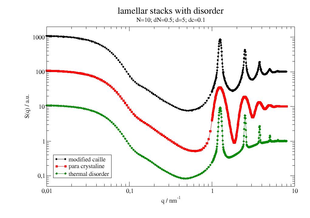
- jscatter.sf.diffuseLamellarStack(q, d, N, dN, kind='caille', dc=0.1)[source]
Bragg peaks and diffuse scattering from lamellar structures.
Lamellar phases are characterized by scattering patterns containing pseudo-Bragg peaks from the layer ordering. Fluctuations of the lamellae cause different kinds of diffuse scattering. See [1] for details and references.
- Parameters:
- qarray
Wavevectors in units nm.
- dfloat
Layer spacing (distance between layers) in units nm.
- Nfloat, int
Number of layers. Actually we use a Poisson distribution with mean N and standard deviation dN. For Large N this is similar to a Gaussian distribution and a valid ditribution for small N.
- dNfloat
Standard deviation from mean describing the width of the Poisson distribution. dN=0 no distribution.
- kind‘difffuse’, ‘para’, ‘caille’
Kind of distortions in the layers
‘diffuse’ : Thermal disorder. [2]
Each layer k fluctuates uncorrelated with an amplitude \(\Delta = (d_k - d)^2\) using a common Debye Waller factor. Uncorrelated fluctuations of layers.
‘para’ : paracrystalline model. [3]
Small fluctuations of layer spacing \(\Delta\) are considered, stacking disorder corresponding to a paracrystal of the second kind. The position of individual fluctuating layers are determined solely by its nearest neighbours.
‘caille’ modified Caille. [4]
Lamellar stacks, the fluctuations are quantified in terms of the flexibility of the membranes dependent on bulk compression modulus B and bending rigidity K of the lamellae. For low dN it approximates normal Caille
- dcfloat
Strength of fluctuations.
‘para’ and ‘diffuse’
Fluctuations of amplitude relative to d. \(dc = \Delta/d\) with \(\Delta = (d_k - d)^2\).
‘caille’
Caille Parameter in modified Caille model.
\[dc = \eta = \frac{\pi kT}{2d(BK)^{1/2}}\]with bulk compression modulus B and bending rigidity K of the lamellae.
- Returns:
- dataArray[q, Sq]
Notes
Multi lamellar structures with disorder. See [1]
thermal disorder
\[S(Q) = N + 2 exp(-\frac{Q^2\Delta^2}{2}) \sum_{k=1}^{N-1} (N-k) cos(kQd)\]paracrystalline theory
\[S(Q) = N + 2 \sum_{k=1}^{N-1} (N-k) cos(kQd) exp(-\frac{k^2Q^2\Delta^2}{2})\]Modified Caillé Theory
\[S(Q) = N + 2 \sum_{k=1}^{N-1} (N-k) cos(kQd) \ exp(-(\frac{Qd}{2\pi})^2 \eta \gamma) (\pi k)^{-(Qd/2\pi)^2 \eta}\]
Distribution of stack sizes (for dN>0):
\[S(Q) = N + \sum_{N_k=pmf(0.001)}^{N_k=pmf(0.999)} w_k S_k(Q)\]using a Poisson distribution with probabilities \(w_k\) for \(N_k\) between percent point function (ppf) 0.001..0.999 .
For reasonable large N the Poisson distribution approximates a Gaussian.
References
[1] (1,2,3)Diffuse scattering from lamellar structures Ian W. Hamley Soft Matter, 18, 711 (2022) DOI: 10.1039/d1sm01758f
[2]Giacovazzo et al Fundamentals of Crystallography, International Union of Crystallography/Oxford University Press, Oxford, 1992. B. D. Cullity and S. R. Stock, Elements of X-ray Diffraction, Prentice Hall, Upper Saddle River, New Jersey, 2001.
[3]I. W. Hamley, Small-Angle Scattering: Theory, Instrumentation, Data and Applications Wiley, Chichester, 2021. R. Hosemann and S. N. Bagchi, Direct Analysis of Diffraction by Matter, North-Holland, Amsterdam, 1962.
[4]R. T. Zhang, R. M. Suter and J. F. Nagle, Phys. Rev. E, 1994, 50, 5047–5060. G. Pabst, M. Rappolt, H. Amenitsch and P. Laggner, Phys. Rev. E, 2000, 62, 4000–4009.
Examples
Comparison of the kind’s. See Fig 2 in [1] .
import jscatter as js
import numpy as np

q = np.r_[js.loglist(0.01,1,100),js.loglist(1,8,300)]
N = 10
d= 5
dN = 0.1
dc = 0.1
Sqcaille = js.sf.diffuseLamellarStack(q, d, N, dN, kind='caille', dc=dc)
Sqpara = js.sf.diffuseLamellarStack(q, d, N, dN, kind='para', dc=dc)
Sqdiffuse = js.sf.diffuseLamellarStack(q, d, N, dN, kind='diffuse', dc=dc)

p = js.grace()
p.plot(q, Sqcaille.Y*10,li=1,le='modified caille')
p.plot(q, Sqpara.Y,li=2,le='para crystaline')
p.plot(q, Sqdiffuse.Y*0.1,li=3,le='thermal disorder')

p.xaxis(scale='l',label='q / nm\S-1')
p.yaxis(scale='l',label='S(q) / a.u.',min=0.05,max=2000)
p.legend(x=0.012,y=0.4)
p.title('lamellar stacks with disorder')
p.subtitle('N=10; dN=0.5; d=5; dc=0.1')
# p.save(js.examples.imagepath+'/diffuseLamellarStack.jpg')
- class jscatter.sf.fccLattice(abc, size, b=None)[source]
Bases:
rhombicLatticeFace centered cubic lattice.
See rhombicLattice for methods.
- Parameters:
- abcfloat
Lattice constant of unit cell.
- size3x integer, integer
A list of integers describing the size in direction of the respective latticeVectors. Size is symmetric around zero in interval [-i,..,i] with length 2i+1. If one integer is given it is used for all 3 dimensions.
- blist of float
Corresponding scattering length of atoms in the unit cell.
- Returns:
- lattice object
.array grid points as numpy array
Examples
import jscatter as js
grid=js.sf.fccLattice(1.2,1)
grid.show(2)
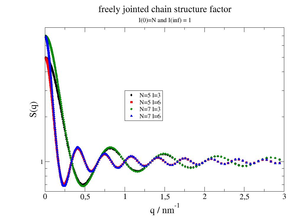
- jscatter.sf.fjc(Q, N, l=2)[source]
Freely jointed chain structure factor.
The structure factor is the structure of N freely jointed beads connected by linkers of equal length where the linkers represent an attractive interaction between neigboring beads leading to a guassian like configuration of a small cluster like a short polymer.
The structure factor is normalized to 1 at large Q and N for Q=0.
- Parameters:
- Qarray
Wavevector in nm.
- Nfloat
Number of beads (homogeneous spheres).
- lfloat
distace between beads in units nm.
- Returns:
- dataArray
Columns [q, sq]
Notes
Added after a remark of Peter Schurtenberger on a meeting to use this as a structure factor.
The structure factor is calculated similar to the freely jointed chain formfactor with thin linkers and for equal point like bead formfactors. See
pearlNecklace()[1].\[S(Q) = 2/N \left[\frac{N}{1-sin(Ql)/Ql}-\frac{N}{2}- \frac{1-(sin(Ql)/Ql)^N}{(1-sin(Ql)/Ql)^2}\cdot\frac{sin(Ql)}{Ql}\right]\]References
[1]Particle scattering factor of pearl necklace chains R. Schweins, K. Huber, Macromol. Symp., 211, 25-42, 2004.
Examples
The high Q modulation corresponds to the bead distance (local order). The low Q describes a random walk of N beads.
import jscatter as js
import numpy as np

q=js.loglist(0.01,3,300)
p=js.grace()
p.plot(js.sf.fjc(q, N=5, l=3),le='N=5 l=3')
p.plot(js.sf.fjc(q, N=5, l=6),le='N=5 l=6')
p.plot(js.sf.fjc(q, N=7, l=3),le='N=7 l=3')
p.plot(js.sf.fjc(q, N=7, l=6),le='N=7 l=6')
p.yaxis(scale='l',label='S(q)',min=0.0001,charsize=1.5)
p.xaxis(scale='n',label='q / nm\S-1',charsize=1.5,min=0,max=3)
p.legend(x=1,y=3)
p.title('freely jointed chain structure factor')
p.subtitle('I(0)=N and I(inf) = 1')
# p.save(js.examples.imagepath+'/fjcsf.jpg')
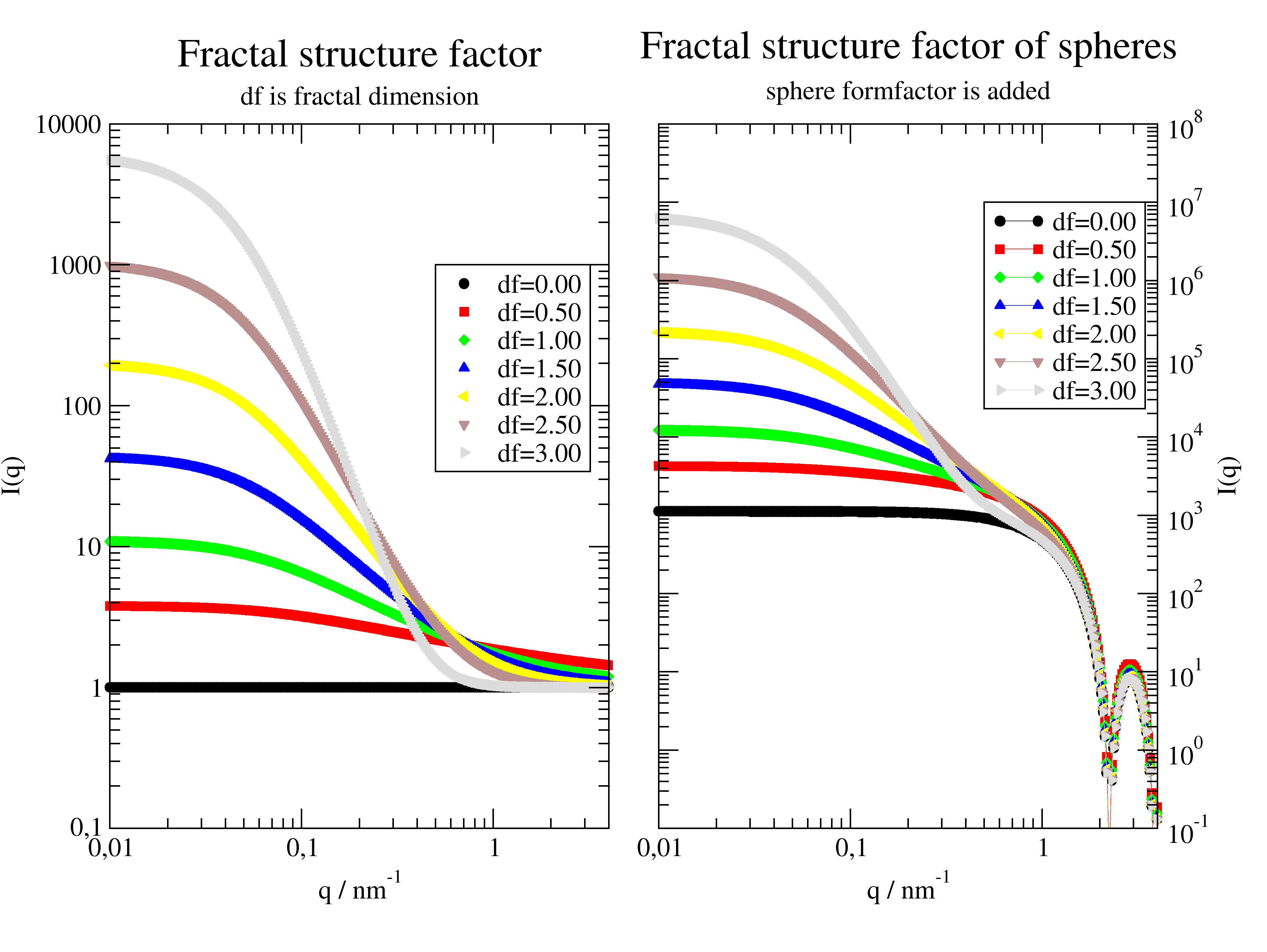
- jscatter.sf.fractal(q, clustersize, particlesize, df=2)[source]
Structure factor of a fractal cluster of particles following Teixeira (mass fractal).
To include the shape/structure of a particle with formfactor F(q) use S(q)*F(q) with particlesize related to the specific formfactor.
- Parameters:
- qarray
Wavevectors in units 1/nm.
- clustersizefloat
Clustersize \(\xi\) in units nm. May be correlated to Rg (see Notes). From [1]: The meaning of \(\xi\) is only qualitative and has to be made precise in any particular situation. Generally speaking, it represents the characteristic distance above which the mass distribution in the sample is no longer described by the fractal law. In practice, it can represent the size of an aggregate or a correlation length in a disordered material.
- particlesizefloat
Particle size in units nm. In [1] it is described as characteristic dimension of individual scatterers. See Notes.
- dffloat, default=2
Hausdorff dimension, \(d_f\) defined as the exponent of the linear dimension R in the relation \(M(R) \propto (R/r_0)^{d_f}\) where M represents the mass and \(r_0\) is the gauge of measurement. See [1].
- Returns:
Notes
The structure factor [1] equ 16 is
\[S(q) = 1 + \frac{d_f\ \Gamma\!(d_f-1)}{[1+1/(q \xi)^2\ ]^{(d_f -1)/2}} \frac{\sin[(d_f-1) \tan^{-1}(q \xi) ]}{(q R_0)^{d_f}}\]At large q the unity term becomes dominant and we get \(S(q)=1\). Accordingly the formfactor of the particles becomes visible.
At intermediate q \(\xi^{-1} < q < r_0^{-1}\) the structure factor reduces to \(S(q)=q^{-d_f}\)
The radius of gyration is related to the cluster size \(\xi\) as \(Rg = d_f(d_f+1) \xi^2/2\) See [1] after equ. 17.
According to [1] the particlesize relates to a characteristic dimension of the particles. The particlesize determines the intersection of the extrapolated power law region with 1 thus the region where the particle structure gets important. The particlesize can be something like the radius of gyration of a Gaussian or collapsed chain, a sphere radius or the mean radius of a protein. It might also be the clustersize of a fractal particle.
In SASview the particlesize is related to the radius of aggregating spheres (or core shell sphere) including a respective formfactor.
References
Examples
Here a fractal structure of a cluster of spheres is shown. The size of the spheres is the particlesize on the cluster. The typical scheme \(I(q)=P(q)S(Q)\) with particle formfactor \(P(q)\) and structure factor \(S(Q)\) is used. The volume and contrast is included in \(P(q)\). Add a background if needed or use a different particle as core-shell sphere.
import jscatter as js
import numpy as np
q=js.loglist(0.01,5,300)

p=js.grace(1.5,1)
p.multi(1,2)
clustersize = 20
particlesize = 2

fq=js.ff.sphere(q,particlesize)
for df in np.r_[0:3:7j]:
    Sq=js.sf.fractal(q, clustersize, particlesize, df=df)
    p[0].plot(Sq,le=f'df={df:.2f}')
    p[1].plot(Sq.X,Sq.Y*fq.Y,li=-1,le=f'df={df:.2f}')

p[0].yaxis(scale='log',label='I(q) ',min=0.1,max=1e4)
p[0].xaxis(scale='log',min=0.01,max=4,label='q / nm\S-1')
p[0].title(r'Fractal structure factor')
p[0].subtitle('df is fractal dimension')
p[0].legend(x=0.5,y=1000)
p[1].yaxis(scale='log',min=0.1,max=1e8,label=['I(q)',1.0,'opposite'],ticklabel=['power',0,1,'opposite'])
p[1].xaxis(scale='log',min=0.01,max=4,label='q / nm\S-1')
p[1].title(r'Fractal structure factor of spheres')
p[1].subtitle('sphere formfactor is added')
p[1].legend(x=0.5,y=1e7)
#p.save(js.examples.imagepath+'/fractalspherecluster.png')
- class jscatter.sf.hcpLattice(ab, size, b=None)[source]
Bases:
rhombicLatticeHexagonal closed packed lattice.
See rhombicLattice for methods.
- Parameters:
- abfloat
Lattice constant of unit cell. ab is distance in hexagonal plane, c = ab* (8/3)**0.5
- size3x integer, integer
A list of integers describing the size in direction of the respective latticeVectors. Size is symmetric around zero in interval [-i,..,i] with length 2i+1. If one integer is given it is used for all 3 dimensions.
- blist of float
Corresponding scattering length of atoms in the unit cell.
- Returns:
- lattice object
.array grid points as numpy array
Examples
import jscatter as js
grid=js.sf.hcpLattice(1.2,[3,3,1])
grid.show(2)
- class jscatter.sf.hex2DLattice(ab, size, b=None)[source]
Bases:
bravaisLatticeSimple 2D hexagonal lattice.
See rhombicLattice for methods.
- Parameters:
- abfloat
Lattice constant of unit cell.
- size2x integer, integer
A list of integers describing the size in direction of the respective latticeVectors. Size is symmetric around zero in interval [-i,..,i] with length 2i+1. If one integer is given it is used for all 3 dimensions.
- blist of float
Corresponding scattering length of atoms in the unit cell.
- Returns:
- lattice object
.array grid points as numpy array
Examples
import jscatter as js
grid=js.sf.hex2DLattice(1.2,1)
grid.show(2)
- class jscatter.sf.hexLattice(ab, c, size, b=None)[source]
Bases:
rhombicLatticeHexagonal lattice.
See rhombicLattice for methods.
- Parameters:
- ab,cfloat
Lattice constant of unit cell. ab is distance in hexagonal plane, c perpendicular. For c/a = (8/3)**0.5 the hcp structure
- size3x integer, integer
A list of integers describing the size in direction of the respective latticeVectors. Size is symmetric around zero in interval [-i,..,i] with length 2i+1. If one integer is given it is used for all 3 dimensions.
- blist of float
Corresponding scattering length of atoms in the unit cell.
- Returns:
- lattice object
.array grid points as numpy array
Examples
import jscatter as js
grid=js.sf.hexLattice(1.,2,[2,2,2])
grid.show(2)
- class jscatter.sf.honeycombLattice(ab, c, size, b=None)[source]
Bases:
rhombicLatticeHoneycomb lattice e.g for graphene.
See rhombicLattice for methods.
- Parameters:
- ab,cfloat
Lattice constants of unit cell. ab is distance between nearest neighbors in honeycomb plane, c perpendicular.
- size3x integer, integer
A list of integers describing the size in direction of the respective latticeVectors. Size is symmetric around zero in interval [-i,..,i] with length 2i+1. If one integer is given it is used for all 3 dimensions.
- blist of float
Corresponding scattering length of atoms in the unit cell.
- Returns:
- lattice object
.array grid points as numpy array
Notes
Similar peak positions as hexagonalLattice with ab*3**0.5 with same peak height for [1,2,n] and smaller peak height in [2,2,n].
Examples
import jscatter as js
grid=js.sf.honeycombLattice(1.,2,[2,2,2],[1,2])
grid.show(5)
- jscatter.sf.hydrodynamicFunct(wavevector, Rh, molarity, intrinsicVisc=None, DsoverD0=None, structureFactor=None, structureFactorArgs=None, numberOfPoints=50, ncpu=-1)[source]
Hydrodynamic function H(q) from hydrodynamic pair interaction of spheres in suspension.
This allows the correction \(D_T(q)=D_{T0}H(q)/S(q)\) for the translational diffusion \(D_T(q)\) coefficient at finite concentration. We use the theory from Beenakker and Mazur [2] as given by Genz [1]. The \(\delta\gamma\)-expansion of Beenakker expresses many body hydrodynamic interaction within the renormalization approach dependent on the structure factor S(q).
- Parameters:
- wavevectorarray
Scattering vector q in units 1/nm.
- Rhfloat
Effective hydrodynamic radius of particles in nm.
- molarityfloat
Molarity in units mol/l.
This overrides a parameter ‘molarity’ in the structureFactorArgs.
Rh and molarity define the hydrodynamic interaction, the volume fraction \(\Phi\) and Ds/D0 for H(Q).
The structure factor may have a radius different from Rh e.g. for attenuated hydrodynamic interactions.
- DsoverD0float
The high Q limit of the hydrodynamic function is for low volume fractions with self diffusion Ds \(\frac{D_s}{D_0}= 1/(1+[\eta] \Phi )\) .
Ds is calculated from molarity and Rh.
This explicit value overrides intrinsic viscosity and calculated Ds/D0.
- structureFactorfunction, None
Structure factor S(q) with S(q=inf)=1.0 recommended.
If structurefactor is None a Percus-Yevick is assumed with molarity and R=Rh.
A function S(q,…) is given as structure factor, which might be an empirical function (e.g. polynominal fit of a measurement). First parameter needs to be wavevector q .
- structureFactorArgsdictionary
Any extra arguments to structureFactor e.g. structFactorArgs={‘gamma’:0.123,R=3,….}
- intrinsicViscfloat
The intrinsic viscosity \([\eta]\) defines the high q limit for the hydrodynamic function. \(\eta(\Phi=0)/\eta(\Phi) = (1-[\eta] \Phi )=D_s/D_0\)
\([\eta]= 2.5\) Einstein result for hard sphere with density 1 g/cm**3
For proteins instead of volume fraction the protein concentration in g/cm³ with typical protein density 1.37 g/cm^3 is often used. Intrinsic Viscosity depends on protein shape (see HYDROPRO).
Typical real values for intrinsicVisc in practical units cm^3/g
sphere 1.76 cm^3/g = 2.5 sphere with protein densityADH 3.9 cm^3/g = 5.5 a tetrameric proteinPGK 4.0 cm^3/g = 5.68 two domains with hinge-> elongatedRnase 3.2 cm^3/g = 4.54 one domain
- numberOfPointsinteger, default 50
Determines number of integration points in equ 5 of ref [1] and therefore accuracy of integration. The typical accuracy of this function is <1e-4 for (H(q) -highQLimit) and <1e-3 for Ds/D0.
- ncpuint, optional
Number of cpus in the pool.
not given or 0 -> all cpus are used
int>0 min (ncpu, mp.cpu_count)
int<0 ncpu not to use
- Returns:
- dataArray
Columns [q, hf, hf1, sf]
q values
hf : hydrodynamic function
hf1 : hydrodynamic function only Q dependent part = H(q) - highQLimit
sf : structure factor S(q) for H(q) calculation
.DsoverD0 : Ds/D0
.DsoverD0_calculated : \(D_s(\Phi)/D_0\)
Notes
As describdes in [1]
\[H(Q) = H_d(Q) + D_s(\Phi)/D_0\]\[H_d(Q)=\frac{3}{2\pi} \int_0^{\infty} dak \frac{sin^2(ak)}{(ak)^2[1+\Phi S_{\gamma}(ak)]} \times \int_{-1}^1 dx(1-x^2)(S(|\mathbf{Q}-\mathbf{k}|)-1)\]\[\frac{D_s(\Phi)}{D_0} = \frac{2}{\pi}\int_0^{\infty} sinc^2(x)[1+\Phi S_{\gamma}(x)]^{-1}\]\(x=cos(\mathbf{Q},\mathbf{k})\) is the angle between vectors Q and k, \(\Phi=4\pi/3a^3/V\) volume fraction of spheres with radius a. \(S_{\gamma}(x)\) is a known function given by Genz [1].
\(D_s/D_0\) from above(equ. 11 in [1]) is valid for volume fractions up to 0.45 (according to ref [3]). With this assumption the deviation of self diffusion \(D_s/D_0\) from Ds/Do=[1-1.73*phi+0.88*phi**2+ O(phi**3)] is smaller 5% for phi<0.2 (10% for phi<0.3)
We allow volume fractions up to 0.55 for the numerical calculation.
References
[2]Beenakker and P. Mazur, Phys. A Stat. Mech. Its Appl. 126, 349 (1984).
[3]Beenakker and P. Mazur, Phys. A Stat. Mech. Its Appl. 120, 388 (1983).
Examples
- class jscatter.sf.lamLattice(a, size, b=None)[source]
Bases:
bravaisLattice1D lamellar lattice.
See rhombicLattice for methods.
- Parameters:
- afloat
Lattice constant of unit cell.
- size1x integer, integer
A list of integers describing the size in direction of the respective latticeVectors. Size is symmetric around zero in interval [-i,..,i] with length 2i+1. If one integer is given it is used for all 3 dimensions.
- blist of float
Corresponding scattering length of atoms in the unit cell.
- Returns:
- lattice object
.array grid points as numpy array
Examples
import jscatter as js
grid=js.sf.lamLattice(1.2,1)
grid.show(2)
- class jscatter.sf.lattice[source]
Bases:
objectCreate an arbitrary lattice.
Please use one of the subclasses below for creation.
pseudorandom, rhombicLattice, bravaisLattice scLattice, bccLattice, fccLattice, diamondLattice, hexLattice, hcpLattice, sqLattice, hexLattice, lamLattice
This base class defines methods valid for all subclasses.
- property X
X coordinates for b!=0
- property XYZ
X,Y,Z coordinates array Nx3 for b!=0
- property XYZall
X,Y,Z coordinates array Nx3
- property Xall
X coordinates
- property Y
Y coordinates for b!=0
- property Yall
Y coordinates
- property Z
Z coordinates for b!=0
- property Zall
Z coordinates
- alongLine(v, R, a=None, length=0, b=1, invert=False)
Set scattering length for points within a long cylinder.
- Parameters:
- a3 x float, default [0,0,0]
Edge point on cylinder axis.
- Rfloat
Radius of cylinder.
- v3 x float
Normal vector along cylinder axis.
- length
Length along cylinder axis.
<0 negative direction
>0 positive direction
=0 infinite both directions
np.inf positive direction, infinite length
np.ninf negative direction, infinite length
- b: float
Scattering length for selected points.
- invertbool
True to invert selection.
Examples
import jscatter as js
import numpy as np
sc=js.sf.scLattice(0.5,30,b=[0])
sc.inCylinder(v=[1,1,1],a=[5,0,5],R=3)
sc.inCylinder(v=[1,-1,1],a=[0,5,0],R=2)
sc.inCylinder(v=[1,0,0],a=[0,-5,-10],length =10,R=2)
sc.inCylinder(v=[0,1,0],a=[5,0,-10],length =10,R=2)
sc.inCylinder(v=[1,0,0],a=[-10,-5,10],length =10,R=2,b=2)
sc.inCylinder(v=[0,1,0],a=[-5,0,10],length =-10,R=2,b=2)
sc.inCylinder(v=[1,0,0],a=[0,5,-10],length =np.NINF,R=2)
sc.show()
- property array
Coordinates and scattering length as array for b!=0
- property b
Scattering length for points with b!=0
- property ball
Scattering length all points
- property dimension
- filter(funktion)[source]
Set lattice points scattering length according to a function.
All points in the lattice are changed for which funktion returns value !=0 (tolerance 1e-12).
- Parameters:
- funktionfunction returning float
Function to set lattice points scattering length. The function is applied with each i point coordinates (array) as input as .points[i,:3]. The return value is the corresponding scattering length.
Examples
# To select points inside of a sphere with radius 5 around [1,1,1]:
from numpy import linalg as la
sc=js.sf.scLattice(0.9,10)
sc.set_b(0)
sc.filter(lambda xyz: 1 if la.norm(xyz-np.r_[1,1,1])<5 else 0)

# sphere with  increase from center
from numpy import linalg as la
sc=js.sf.scLattice(0.9,10)
sc.set_b(0)
sc.filter(lambda xyz: 2*(la.norm(xyz)) if la.norm(xyz)<5 else 0)
fig=sc.show()
- inCylinder(v, R, a=None, length=0, b=1, invert=False)[source]
Set scattering length for points within a long cylinder.
- Parameters:
- a3 x float, default [0,0,0]
Edge point on cylinder axis.
- Rfloat
Radius of cylinder.
- v3 x float
Normal vector along cylinder axis.
- length
Length along cylinder axis.
<0 negative direction
>0 positive direction
=0 infinite both directions
np.inf positive direction, infinite length
np.ninf negative direction, infinite length
- b: float
Scattering length for selected points.
- invertbool
True to invert selection.
Examples
import jscatter as js
import numpy as np
sc=js.sf.scLattice(0.5,30,b=[0])
sc.inCylinder(v=[1,1,1],a=[5,0,5],R=3)
sc.inCylinder(v=[1,-1,1],a=[0,5,0],R=2)
sc.inCylinder(v=[1,0,0],a=[0,-5,-10],length =10,R=2)
sc.inCylinder(v=[0,1,0],a=[5,0,-10],length =10,R=2)
sc.inCylinder(v=[1,0,0],a=[-10,-5,10],length =10,R=2,b=2)
sc.inCylinder(v=[0,1,0],a=[-5,0,10],length =-10,R=2,b=2)
sc.inCylinder(v=[1,0,0],a=[0,5,-10],length =np.NINF,R=2)
sc.show()
- inEllipsoid(abc, rotation=None, center=None, b=1, invert=False)[source]
Set scattering length for points in ellipsoid.
- Parameters:
- abc: [float,float,float]
Principal semi axes length of the ellipsoid.
- rotationscipy.spatial.transform.Rotation object
Rotation describing the rotation semi axes rotation from the cartesian axes. e.g. scipy.spatial.transform.Rotation.from_rotvec([np.pi/4, 0, 0])
- center3 x float, default [0,0,0]
Center of the sphere.
- b: float
Scattering length for selected points.
- invertbool
True to invert selection.
Examples
import jscatter as js
from scipy.spatial.transform import Rotation as R
sc=js.sf.scLattice(0.5,30,b=[0])
sc.inEllipsoid(abc=[3,1,12],b=1)
sc.show()
sc.inEllipsoid(abc=[3,1,12],rotation=R.from_euler('X',45,degrees=True),b=2)
sc.show()
sc.inEllipsoid(abc=[3,1,12],rotation=R.from_euler('XY',[45,90],degrees=True),b=3)
sc.show()
- inParallelepiped(v1, v2, v3, corner=None, b=1, invert=False)[source]
Set scattering length for points in parallelepiped.
- Parameters:
- corner3x float
Corner of parallelepiped
- v1,v2,v3each 3x float
Vectors from origin to 3 corners that define the parallelepiped.
- b: float
Scattering length for selected points.
- invertbool
Invert selection
Examples
import jscatter as js
sc=js.sf.scLattice(0.2,10,b=[0])
sc.inParallelepiped([1,0,0],[0,1,0],[0,0,1],[0,0,0],1)
sc.show()
sc=js.sf.scLattice(0.1,30,b=[0])
sc.inParallelepiped([1,1,0],[0,1,1],[1,0,1],[-1,-1,-1],2)
sc.show()
- inSphere(R, center=None, b=1, invert=False)[source]
Set scattering length for points in sphere.
- Parameters:
- center3 x float, default [0,0,0]
Center of the sphere.
- R: float
Radius of sphere around origin.
- b: float
Scattering length for selected points.
- invertbool
True to invert selection.
Examples
import jscatter as js
sc=js.sf.scLattice(1,15,b=[0])
sc.inSphere(6,[2,2,2],b=1)
sc.show()
sc.inSphere(6,[-2,-2,-2],b=2)
sc.show()

sc=js.sf.scLattice(0.8,20,b=[0])
sc.inSphere(3,[2,2,2],b=1)
sc.inSphere(3,[-2,-2,-2],b=1)
sc.show()

sc=js.sf.scLattice(0.8,20,b=[0])
sc.inSphere(3,[2,2,2],b=1)
sc.inSphere(4,[0,0,0],b=2)
sc.show()
- isLattice = True
- property lastSelection
Give last selection from filter, inSphere, inCylinder, inEllipsoid, planeSide, inParallelepiped.
- move(vector)[source]
Move all points by vector.
- Parameters:
- vectorlist of 3 float or array
Vector to shift the points.
- property nonzerob
Mask of nonzero b.
- planeSide(vector, center=None, b=1, invert=False)[source]
Set scattering length for points on one side of a plane.
- Parameters:
- center3x float, default [0,0,0]
Point in plane.
- vectorlist 3x float
Vector perpendicular to plane.
- b: float
Scattering length for selected points.
- invertbool
False choose points at origin side. True other side.
Examples
sc=js.sf.scLattice(1,10,b=[0])
sc.planeSide([1,1,1],[3,3,3],1)
sc.show()
sc.planeSide([-1,-1,0],3)
sc.show()
- property points
Points with scattering length !=0
grid._points contains all Nx[x,y,z,b]
- prune(select=None)[source]
Prune lattice to reduced number of points (in place).
- Parameters:
- selectbool array xN or function
A bool array of length grid points to keep only points that are true or a bool function that is evaluated for each [x,y,z,b] evaluating to True. By default all pounts with b=0 are removed.
Examples
grid.prune(grid.ball>0)  # bool array
grid.prune(lambda a:a[3]>0)  # function
- rotate(axis, angle)[source]
Rotate points in lattice around axis by angle.
- Parameters:
- axislist 3xfloat
Axis of rotation
- angle
Rotation angle in rad
- set_b(b)[source]
Set all points to given scattering length.
- Parameters:
- bfloat or array length points
- set_bsel(b, select)[source]
Set b of all points (including points with b==0) according to selection.
To access all points us the properties grid.??all which contains all coordinates and b.
- Parameters:
- bfloat or array length _points
Scattering length
- selectbool array
Selection array of len(grid.ball)
Examples
grid.set_ball(1, grid.Xall > 0)
- property shape
Shape for points with b!=0
- property shapeall
Shape for points with b!=0
- show(R=None, cmap='rainbow', fig=None, ax=None, atomsize=1)[source]
Show the lattice in matplotlib with scattering length color coded.
- Parameters:
- Rfloat,None
Radius around origin to show.
- cmapcolormap
Colormap. E.g. ‘rainbow’, ‘winter’,’autumn’,’gray’ to color atoms according to their scattering length b. Use js.mpl.showColors() for all possibilities.
- figmatplotlib Figure
Figure to plot in. If None a new figure is created.
- axAxes
If given this axes is used for plotting.
- atomsizefloat
Sphere size of the atoms. Unfortunately matplotlib does not scale the point size when zooming.
- Returns:
- fig handle
Notes
If the three dimensional overlap is wrong this is due to matplotlib. matplotlib is not a real 3D graphic program.
- property type
Returns type of the lattice
- class jscatter.sf.latticeFromCIF(structure, size=[1, 1, 1], typ='x')[source]
Bases:
rhombicLatticeCreate lattice as defined in CIF (Crystallographic Information Format) file or a pymatgen structure.
- Parameters:
- structurestr, pymatgen.structure
Filename of the CIF file or structure read by pymatgen as
structure = pymatgen.core.Structure.from_file(js.examples.datapath+'/1011053.cif')- typ‘xray’,’neutron’
scattering length for coherent xray or neutron scattering.
- size3x int
Size of the lattice in direction of lattice vectors
Notes
Pymatgen (Python Materials Genomics) is a robust, open-source Python library for materials analysis [1]. See Pymatgen
# Simply install by
pip install pymatgen
CIF files can be found in the Crystallography Open Database
Pymatgen allows site occupancy which is taken here into account as average scattering length per site.
Pymatgen allows reading of CIF files or to get directly a structure from Materials Project or Crystallography Open Database .
Look at Examples
from pymatgen.ext.cod import COD
cod = COD()
# SiC silicon carbide (carborundum or Moissanite)
sic = cod.get_structure_by_id(1011053)
sicc=js.sf.latticeFromCIF(sic)
# silicon
si = cod.get_structure_by_id(9008566)
If Bragg peaks or reciprocal lattice points are missing try to increase the size parameter as these points might belong to higher order lattice planes. E.g. for SiC (silicon carbide) the second peak at \(2\theta=35.6^{\circ}\) belongs to hkl = 006 or the 8th order peak at \(2\theta=60.1^{\circ}\) belongs to hkl = 108 .
References
[1]Python Materials Genomics (pymatgen) : A Robust, Open-Source Python Library for Materials Analysis. Ong et al Computational Materials Science, 2013, 68, 314–319. doi:10.1016/j.commatsci.2012.10.028
Examples
The example is for silicon carbide. Please compare to Moissanite
import jscatter as js
import pymatgen
siliconcarbide = pymatgen.core.Structure.from_file(js.examples.datapath+'/1011053.cif')
sic=js.sf.latticeFromCIF(siliconcarbide)
sic.getScatteringAngle(wavelength=0.13141,size=13)

from pymatgen.ext.cod import COD
cod = COD()
# 3C-SiC silicon carbide (carborundum or Moissanite)
siliconcarbide = cod.get_structure_by_id(1011031)
sic=js.sf.latticeFromCIF(siliconcarbide)
sic.getScatteringAngle(size=13)
- class jscatter.sf.latticeFromMDA(atoms, latticeVectors=None, size=[1, 1, 1], typ='x')[source]
Bases:
rhombicLatticeCreate lattice with a unit cell defined from MDAnalysis universe atomgroup.
- Parameters:
- atomsMDAnalysis universe atomgroup
Atomsgroup of universe created with MDAnalysis or bio.scatteringUniverse
- latticeVectors3x array(3)
Lattice vectors spanning the unit cell enclosing the atomgroup.
- typ‘xray’,’neutron’
scattering length for coherent xray or neutron scattering.
- size3x int
Size of the lattice in direction of lattice vectors
Examples
We look at an alpha helix ordered in a hexagonal lattice. We need first to orient the helix to fit into the lattice with defined orientation. The aim is to calculate the structure factor.
import jscatter as js
import numpy as np
from scipy.spatial.transform import Rotation as Rot
from scipy import linalg as la

uniR=js.bio.scatteringUniverse(js.examples.datapath+'/arg61.pdb',addHydrogen=False)

# rotate the helix parallel to the Z axis
uniR.atoms.positions = uniR.atoms.positions-uniR.atoms.center_of_geometry()
up = uniR.select_atoms('name CA and resnum 2-8')
vup = up.positions.mean(axis=0)
rotv = np.cross(vup,[0,0,1])
rotv = rotv/la.norm(rotv)
r = Rot.from_rotvec( -np.arctan(la.norm(vup[:2])/vup[2]) * rotv)
uniR.atoms.positions =  uniR.atoms.positions @ r.as_matrix()
uniR.atoms.positions = uniR.atoms.positions - np.r_[0,0,uniR.atoms.positions[:,2].min()]
# uniR.view(viewer='pymol')

# define lattice constant
hex_c = 13  # bit larger then helix
hex_a = 2   # bit larger than radius

# get lattice vectors
v1,v2,v3 = js.sf.hexLattice(hex_a,hex_c,1).latticeVectors

# create lattice with universe atoms in unit cell
PLA = js.sf.latticeFromMDA(uniR.atoms,[v1,v2,v3],size=[1,1, 0])
# PLA.show()

# now we use latticeStructureFactor to calculate the lattice structure factor
p = js.grace()
p.title('poly arginine alpha helix in hexagonal lattice')
p.subtitle('hexagonal peak intensity modified by unit cell atoms')

q = np.r_[0.1:25:1000j]
sf = js.sf.latticeStructureFactor(q, lattice=PLA,domainsize=60, rmsd=0.02, lg=1, hklmax=6,wavelength=0.15406)
p.plot(sf.X,sf.Y + 0.03,sy=[1,0.3,1],li=1)

p.xaxis(label='q / nm\S-1',scale='log',min=0.1,max=20)
p.yaxis(label='I(q)',scale='log',min=0.02,max=5)
p.text(string='lamellar peaks',x=0.7,y=1)
p.text(string='hexagonal peaks',x=3.6,y=0.4)
# p.save(js.examples.imagepath+'/PLALatticeSf.jpg',size=[600,600])
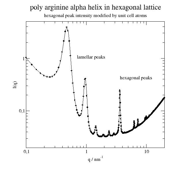
- jscatter.sf.latticeStructureFactor(q, lattice=None, domainsize=1000, asym=0, lg=1, rmsd=0.02, beta=None, hklmax=7, c=1.0, wavelength=None, corrections=[])[source]
Radial structure factor S(q) in powder average of a crystal lattice with particle asymmetry, Debye-Waller factor, diffusive scattering and broadening due to domain size.
To get the full scattering the formfactor needs to be included (See Notes and Examples).
1-3 dimensional lattice structures with basis containing multiple atoms (see lattice).
For 1D and 2D a corresponding 1D or 2D formfactor has to be used. See Notes.
Self absorption and self extinction are not included. Polarisation and Lorentz correction are optional.
How to fit see last example latticeStructureFactor as a fit model .
- Parameters:
- qarray float
Norm of wavevectors in inverse units of lattice constant, units 1/nm
- domainsizefloat
Domainsize of the crystal, units as lattice constant of lattice. According to Debye-Scherrer equation \(fwhm=2\pi/domainsize\) the peak width is determined [2].
- latticelattice object
The crystal structure as defined in a lattice object. The size of the lattice is ignored. One of rhombicLattice, bravaisLattice, scLattice, bccLattice, fccLattice, diamondLattice, hexLattice, hcpLattice. See respective definitions. rhombicLattice can be used to define arbitrary shaped particles in the unit cell. See examples.
- lgfloat, default = 1
Lorenzian/Gaussian fraction describes the contributions of Gaussian and Lorenzian shape in peak shape (Voigt function).
lorenzian/gaussian >> 1 lorenzian,
lorenzian/gaussian ~ 1 central part gaussian, outside lorenzian wings
lorenzian/gaussian << 1 gaussian
- asymfloat, default=0
Asymmetry factor in sigmoidal as \(2fwhm/(1+e^{asym*(x-center)})\) For asym=0 the Voigt is symmetric with fwhm. See formel.voigt .
- rmsdfloat, [3xfloat], default=0.02
Root mean square displacement \(rmsd=<u^2>^{0.5}\) determining the Debye Waller factor. Units as domainsize and lattice units.
float : The Debye Waller factor is used as \(DW(Q)=e^{-Q^2 rmsd^2 }=e^{-Q^2 u^2 }\)
3xfloat : Assuming different displacements along the lattice vectors. In general a matrix describes anisotropic displacements according to Kronenburg [6]. We allow here anisotropic displacements \(rmsd = (u_1,u_2,u_3)\) along the .latticeVectors \(v_i\) with \(DW_{hkl}(Q)=exp(-q_{hkl} U q_{hkl})\) and \(U=diag(u1,u2,u3)\). See Notes.
- betafloat, None, dataArray
Asymmetry factor of the formfactor or reduction due to polydispersity.
None beta=1, No beta assumed (spherical symmetric formfactor, no polydispersity)
dataArray explicitly given as dataArray with beta in .Y column. Missing values are interpolated.
An approximation for polydisperse beta can be found in [1] equ.17. This can be realized by beta=js.dA(np.vstack(q,np.exp(-(q*sr*R)**2))) with sr as relative standard deviation of gaussian distribution of the size R.
See .formfactor for different formfactors which explicit calculation of beta.
- hklmaxint
Maximum order of the Bragg peaks to include.
- cfloat, default=1
Porod constant. See 3.8 in [1].
- wavelengthfloat, default = None
Wavelength of the measurement in units nm. If None .Braggtheta is not calculated. For Xray Cu K_a it is 0.15406 nm.
- correctionslist, default=[]
List of corrections to apply, which depend on the measurement type/geometry [5]. \(\theta\) is here the scattering angle (not \(2\theta\) as in diffraction is used)
‘TP’ Thompson polarisation correction \((1+cos^2(\theta)/2)\) for electromagnetic scattering as Xrays [4]. For small angle scattering this is negligible but valid. For polarised beams the polarisation has to be included.
‘lh’ likelihood of a crystallite being in diffraction position \(cos(\theta/2)\).
‘LC’ Lorentz correction \(\sin(\theta)^{-1}\) due to integration over the width of reciprocal Bragg peaks due to lattice imperfections and the width of the incoming beam. Use for Debye-Scherrer (powder of crystallites) diffraction.
‘area’ the intensity for a given diffraction peak is recorded on a narrow strip of photographic film instead of over the entire diffraction cone \(\sin(\theta)^{-1}\).
‘all’ common Lorentz and polarisation correction powder measurements of crystalline material. Use all from above. NOT for flat transmission geometry (typical SAS) or non crystallite . Corresponds to \((1+cos^2(\theta)/2)/sin^2(\theta/2)/sin(\theta/2)\).
The correction for the pixel area presented to scattering solid angle is included in sasImage in 2D also correcting for offset detector positions of a flat detector, which cannot use the scattering angle \(\theta\) as the geometry changes.
- Returns:
- dataArray
Columns [q, Sq, DW, beta, Z0q, correction, theta]
q wavevector
Sq = S(q) = (1+beta(q)*(Z0(q)-1)*DW(q))*correction structure factor
DW(q) Debye-Waller factor with (1-DW)=diffusive scattering.
beta(q) asymmetry factor of the formfactor.
Z0q lattice factor Z0(q)
optional
correction [optional] factor polarisation from Thompson scattering
theta scattering angle
Attributes
.q_hkl peak positions
.fhkl symmetry factor
.mhkl multiplicity
.Braggtheta Bragg angles
Notes
Analytical expressions for the scattering functions of atomic crystals and ordered mesoscopic materials . Ordered structures in 3D (fcc, bcc, hcp, sc), 2D (hex, sq) and lamellar structures are considered. The expressions take into account particle size distributions and lattice point deviations, domain size, core/shell structures, as well as peak shapes varying analytically between Lorentzian and Gaussian functions. The expressions allow one to quantitatively describe high-resolution synchrotron small-angle X-ray (SAXS) and neutron scattering (SANS) curves from lipid and block copolymer lyotropic phases, core/shell nanoparticle superstructures, ordered nanocomposites, ordered mesoporous materials and atomic crystal structures (see AgBe example).
The scattering intensity of a crystal domain in powder average is for isotropic scattering particles
\[I(q) = {\Delta\rho}^2 n P(q) S(q)\]with
\(\Delta\rho\) scattering length difference between matrix and particles
\(n\) number density (of elementary cells)
\(P(q)\) radial averaged form factor of the particles
\(S(q)\) structure factor \(S(q)\)
Separation of structure factor and formfactor \(P(q)\) in 3D is possible under the assumption of isotropic oriented particles. Including polydispersity of particles as size polydispersity or anisotropic shape like ellipsoids (but still isotropic orientation) leads to the correction \(\beta(q)\). \(\beta(q)\) does not account for non isotropic alignment as e.g.in lyotropic phases of cylinders.
For 1D and 2D structure factor a corresponding formfactor with reduced dimesionlity that factorizes has to be used. Explicitly e.g. using a 3D formfactor as a sphere in 2D hexagonal lattice is wrong. Approximately a very long oriented cylinder might be used, but a flat disc (2D) is correct.
The above structure factor is [1] :
\[S(q)=1+ \beta(q)(Z_0(q)-1)*DW(q)\]with
\(\beta(q)=<F(q)>^2/<F(q)^2>\) as asymmetry factor [3] dependent on the scattering amplitude \(F(q)\) and particle polydispersity
\(DW(q)\) Debye Waller factor
The lattice factor is [1] :
\[Z_0(q) = \frac{(2\pi)^{d-1}c}{nv_dq^{d-1}} \sum\limits_{hkl}m_{hkl}f_{hkl}^2L_{hkl}(q)\]with
\(n\) number of particles per unit cell
\(f_{hkl}\) unit cell structure factor that takes into account symmetry-related extinction rules
\(v_d\) volume of the d-dimensional unit cell
\(hkl\) reflections
\(m_{hkl}\) peak multiplicity
\(c\) Porod constant \(\simeq 1\)
The structure factors of lattices of anisotropic particles with strong orientation like ordered cylinders can be calculated using only the lattice factor and using a unit cell with additional dummy atoms representing the asymmetric particle. The unit cell structure factor represents in these cases the formfactor amplitude in direction of Bragg peaks. See later example Lyotropic hexagonal phase.
Unit cell structure factors \(f_{hkl}\) are normalized that the lattice factor is normalized for infinite q to 1. With i as unit cell atoms at fractional position in the unit cell \([x_i,y_i,z_i]\) and scattering amplitude \(b_i\) we get :
\[f_{hkl}^2 = \big(\sum_i b_i e^{-2\pi (hx_i+ky_i+lz_i)}\big)^2 / \sum_i b_i^2\]We use a Voigt function for the peak shape \(L_{hkl}(q)\) (see formel.voigt).
DW (isotropic) is a Debye Waller like factor as \(DW(q)=e^{-q^2<u^2>}\) leading to a reduction of scattered intensity and diffusive scattering. It has contributions from thermal lattice disorder ( DW factor with 1/3 factor in 3D), surface roughness and size polydispersity.
DW anisotropic: in case of anisotropic Debye Waller factor according to Kronenburg [6] (beta==1):
\[S(q)= \frac{(2\pi)^{d-1}c}{nv_dq^{d-1}} \sum\limits_{hkl} DW_{hkl}(q) m_{hkl}f_{hkl}^2L_{hkl}(q) + (1-\sum\limits_{hkl}DW_{hkl}(q)/N)\]with \(DW_{hkl}(q) = exp(-q_{hkl}Uq_{hkl})\), N as number of hkl. \(q_{hkl}\) is the scattering vector in hkl direction and \(U\) the diagonal matrix of squared displacements in direction of the basis lattice vectors.
\(\beta(q)\) is not included in this case as no particle orientational average is required.
- For the limiting behavior q->0 see the discussion in [1] in 3.9. :
“… The zero-order peak is not explicitly considered because of the q^(1-dim) singularity and because its intensity depends also on the scattering length difference between the lattice inside and outside… Due to the singularity and since structural features on length scales d > a, such as packing defects, grain boundaries or fluctuations decaying on larger length scales are only indirectly considered via the domain size D, eq 30 is not expected to give good agreement with experimentally determined scattering curves in the range of scattering vectors q < 2π/a. However, for q > 2π/a, this approach describes remarkably well experimentally measured high-resolution scattering curves….”
A good description of the real scattering for low Q is shown in example A nano cube build of different lattices for the example of a cube crystal domain..
References
[1] (1,2,3,4,5)Scattering curves of ordered mesoscopic materials. Förster, S. et al. J. Phys. Chem. B 109, 1347–1360 (2005).
[2]Patterson, A. The Scherrer Formula for X-Ray Particle Size Determination Phys. Rev. 56 (10): 978–982 (1939) doi:10.1103/PhysRev.56.978.
[3]Kotlarchyk and S.-H. Chen, J. Chem. Phys. 79, 2461 (1983).1
[5]Modern Physical Metallurgy chapter 5 Characterization and Analysis R.E.SmallmanA.H.W.Ngan https://doi.org/10.1016/B978-0-08-098204-5.00005-5
Examples
Structure factor for hexagonal lattice dependent on rmsd.
import jscatter as js
import numpy as np
q = np.r_[0.02:1:800j]
a = 50.
R=15
sr=0.1
p = js.grace()
beta=js.dA(np.vstack([q,np.exp(-(q*sr*R)**2)]))
p.title('structure factor for hexagonal 2D lattice with a={0} nm'.format(a))
p.subtitle('with diffusive scattering and asymmetry factor beta')
for i,rmsd in enumerate([1., 3., 10., 30.],1):
    grid=js.sf.hexLattice(50,5,5)
    hex = js.sf.latticeStructureFactor(q, rmsd=rmsd, domainsize=500., beta=beta,lattice=grid)
    p.plot(hex, li=[1, 2, i], sy=0, le='rmsd=$rmsd')
    p.plot(hex.X,1-hex._DW, li=[3, 2, i], sy=0)
p.plot(hex.X, hex._beta, li=[2, 2, i], sy=0, le='beta')
p.text(r'broken lines \nshow diffusive scattering',x=0.4,y=6)
p.yaxis(label='S(q)')
p.xaxis(label='q / nm')
p.legend(x=0.6,y=4)
Comparison of sc, bcc, fcc for same cubic unit cell size to demonstrate selection rules.
import jscatter as js
import numpy as np
q=np.r_[js.loglist(0.1,3,200),3:40:800j]
unitcelllength=1.5
N=2
R=0.5
sr=0.1
beta=js.dA(np.vstack([q,np.exp(-(q*sr*R)**2)]))
rmsd=0.02
#
scgrid= js.lattice.scLattice(unitcelllength,N)
sc=js.sf.latticeStructureFactor(q, rmsd=rmsd, domainsize=50., beta=beta,lattice=scgrid)
bccgrid= js.lattice.bccLattice(unitcelllength,N)
bcc=js.sf.latticeStructureFactor(q, rmsd=rmsd, domainsize=50., beta=beta,lattice=bccgrid)
fccgrid= js.lattice.fccLattice(unitcelllength,N)
fcc=js.sf.latticeStructureFactor(q, rmsd=rmsd, domainsize=50., beta=beta,lattice=fccgrid)
#
p=js.grace()
p.plot(sc,legend='sc')
p.plot(bcc,legend='bcc')
p.plot(fcc,legend='fcc')
p.yaxis(label='S(q)',scale='l',max=50,min=0.05)
p.xaxis(label='q / nm',scale='l',max=50,min=0.5)
p.legend(x=1,y=30,charsize=1.5)
# p.save(js.examples.imagepath+'/latticeStructureFactor2.jpg')
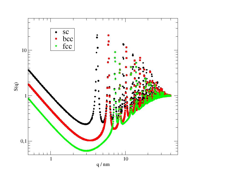
A realistic example of a calibration measurement with AgBe. We load the cif file of the crystal structure to build the lattice and find excellent agreement. According to materialsproject.org calculated XRD tends to underestimate lattice parameters.
For AgBe the first peak is found at 1.07 and lamellar peaks go up to 12.9 because of the Ag atoms in lamellar stack. The broad strong peak 13.7-14 (and upwards) is caused by multiple not lamellar peaks from structure of Be atoms.
import jscatter as js
import numpy as np
#
# Look at raw calibration measurement
calibration = js.sas.sasImage(js.examples.datapath+'/calibration.tiff')
bc=calibration.center
calibration.mask4Polygon([bc[0]+8,bc[1]],[bc[0]-8,bc[1]],[bc[0]-8+60,0],[bc[0]+8+60,0])
# mask center
calibration.maskCircle(calibration.center, 18)
# mask outside shadow
calibration.maskCircle([500,320], 280,invert=True)
# calibration.show(axis='pixel',scale='log')
cal=calibration.radialAverage()
# lattice from crystallographic data in cif file.
agbe=js.sf.latticeFromCIF(js.examples.datapath + '/1507774.cif',size=[0,0,0])
sfagbe=js.sf.latticeStructureFactor(np.r_[cal.X, cal.X[-1]:20:30j], lattice=agbe,
                                   domainsize=50, rmsd=0.001, lg=1, hklmax=17,wavelength=0.15406)

p=js.grace()
p.plot(cal)
# add scaling and background (because of unscaled raw data)
p.plot(sfagbe.X,190*sfagbe.Y+1.9,sy=0,li=[1,3,4])
p.yaxis(scale='log',label='I(q) / counts/pixel')
p.xaxis(scale='log',label='q / nm|S-1',min=0.7,max=20)
p.title('AgBe reference measurements')
# p.save(js.examples.imagepath+'/latticeStructureFactor.jpg')
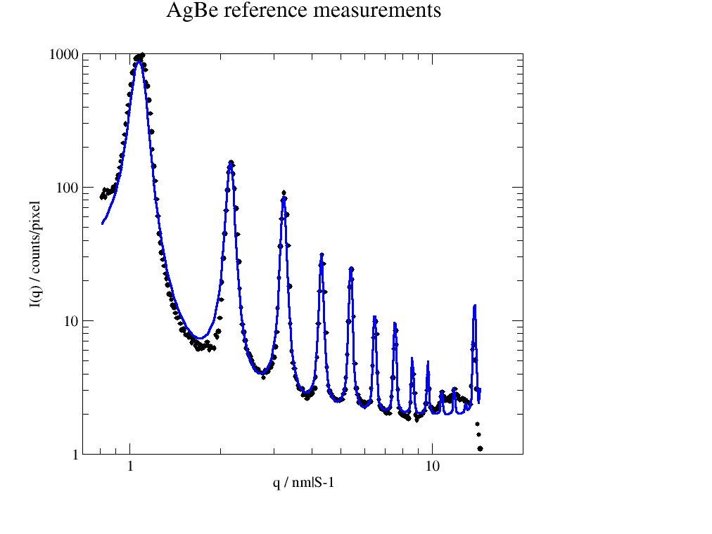
Anisotropic Debye Waller factor
We look at a hexagonal lyotropic phase of long cylinders (e.g. micelles) and calculate the structure factor.
The formfactor amplitude influence is missing here. This cannot be included by multiplying with the orientational averaged fomfactor as the cylinders keep relative orientation. To include the formfactor amplitude look at the next example
The dislocation along the cylinder axis direction might be larger than within the hexagonal plane. We might have dislocations and length polydispersity leading to different rmsd in crystal orientations.
import jscatter as js
import numpy as np
q = js.loglist(0.03,20,800)
#
grid = js.lattice.hexLattice(3,25,5)
# stronger rmsd along cylinder axis
hex = js.sf.latticeStructureFactor(q, rmsd=[0.01,0.01,1.5], domainsize=50.,lattice=grid)
p=js.grace()
#p.plot(hex0)
p.plot(hex,sy=0,li=[1,2,1])
p.yaxis(scale='log',label='I(q) / counts/pixel',min=0.1,max=200)
p.xaxis(scale='log',label='q / nm|S-1',min=0.05,max=20)  #
p.subtitle(r'Structure factor of a hexagonal lattice \nfilled with long cylinders')
p.text('lamellar plane peaks ',x=0.15,y=80)
p.text('hexagonal peaks ',x=2,y=10)
# p.save(js.examples.imagepath+'/hexLyotropicPhaseWithDisorder.jpg')
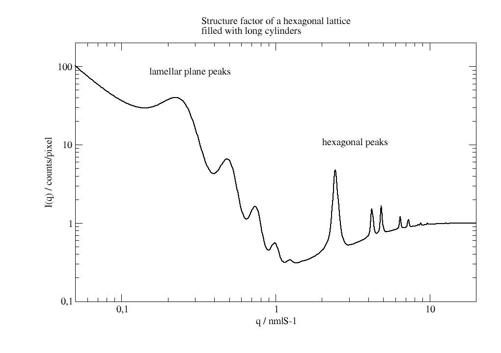
Lyotropic hexagonal phase in 3D Opposite to the above we include here the cylinder shape in the hexagonal lyotropic unit cell. We add in the unit cell a dummy atom representation of the cylinder with good enough resolution. This is used to calculate the \(f_{hkl}^2\) which represents the formfactor amplitude in hkl direction.
This type of scattering is often described as 2D hexagonal lattice with 2D disc formfactor assuming an infinite long cylinder. Here we could add ellipsoids or other anisotropic shapes and inhomogeneous particles.
We explicitly observe here suppression of higher order hexagonal peaks. The first hexagonal peak at \(2.46 nm^{-1}\) show a shift due to the strong decrease on the ff amplitude. The general increase is due to diffuse scattering.
import jscatter as js
import numpy as np
q = js.loglist(0.03,20,800)

# create lattice vectors in a simple way
hexgrid = js.sf.hexLattice(3,20,1)

# create cylinder with atoms in much shorter distance than hex lattice
cylinder = js.sf.scLattice(0.3,[6, 6, 30])
cylinder.move([0,0,9])
cylinder.inCylinder(v=[0,0,1], R=0.5, a=[0,0,0.5], length=15, b=0, invert=True)

# Convert the cylinder points coordinates to
# fractional unit cell coordinates of the hexagonal lattice
mat = np.linalg.inv(hexgrid.latticeVectors).T
cellAtoms = mat @ cylinder.XYZ.T

# create lattice with cylinder unit cell atoms
grid=js.sf.rhombicLattice(latticeVectors=hexgrid.latticeVectors,
                           size=[1,1,1],
                           unitCellAtoms=cellAtoms.T,
                           b=cylinder.b)
q = np.r_[0.1:25:1000j]
hex = js.sf.latticeStructureFactor(q,rmsd=  [0.001,0.001,1.], domainsize=50, lattice=hexgrid)
hexff = js.sf.latticeStructureFactor(q,rmsd=[0.001,0.001,1.], domainsize=50, lattice=grid)
ffcylinder = js.ff.cloudScattering(q,cloud=cylinder)

p=js.grace()
p.plot(hex,sy=0,li=[1,1,1],le='structurefactor 1 atom unit cell')
p.plot(hexff, sy=0,li=[1,3,2], le='+ cylinder in unit cell ')
p.plot(ffcylinder.X, ffcylinder.Y *100 , sy=0, li=[3,1.5,4], le='cyl. formfactor')

p.yaxis(scale='log',label='I(q)',min=0.03,max=200)
p.xaxis(scale='log',label='q / nm\S-1',min=0.05,max=20)  #
p.title(r'Scattering of a hexagonal lattice')
p.subtitle(r'filled with long cylinders, comparison with formfactor')
p.text('lamellar plane peaks ',x=0.1,y=0.5)
p.text(r'hexagonal peaks \nsuppressed by \nformfactor',x=3,y=10)
p.legend(x=0.7,y=200)
# p.save(js.examples.imagepath+'/hexLyotropicPhaseWithDisorder2.jpg')
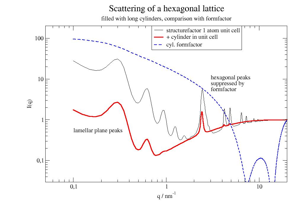
latticeStructureFactor as a fit model We include the possibility of polydispersity.
We use a hexagonal lattice with small hex_a lattice constant and large hex_c to mimic a lamellar structure with lattice constant 5.833 nm as found for AgBe with main scattering coming from Ag atoms in a plane (z=0). The fit results are not as good as the above AgBe example. The fit can be improved limiting it to Q<7. This highlights the importance of the atom distribution in the unit cell in the example above.
import jscatter as js

# smearing even for SAXS here with a single width (for one of our SAXS machines).
fbeam_12=js.sas.prepareBeamProfile(0.035)

def hexSF(q, hex_c,hex_a, domainsize, rmsd,):
   # hexagonal structure factor
    # first make a lattice (size is later ignored)
    hex = js.sf.hexLattice(ab=hex_a,c=hex_c,size=5)
    # then calculate the structure factor and return it
    sf = js.sf.latticeStructureFactor(q=q, lattice=hex, domainsize=domainsize,
                                      hklmax=17, rmsd=rmsd, wavelength=0.15406)
    return sf

# This includes a beamprofile for smearing (may be ommited)
@js.sas.smear(beamProfile=fbeam_12)
def hexmodel(q, hex_c,hex_a,dc, domainsize, rmsd, bgr, I0):
    if dc >0:
        # include a polydispersity in lattice constant, or wavelength or whatever is reasonable
        # also multiple parameters are possible using mPDA
        result  = js.formel.pDA(hexSF, dc, 'hex_c',q=q,hex_a=hex_a,hex_c=hex_c,domainsize=domainsize,rmsd=rmsd)
    else:
        # no polydispersity, do it direct
        result = hexSF(q=q,hex_a=hex_a,hex_c=hex_c,domainsize=domainsize,rmsd=rmsd)
    result.Y=I0*result.Y+bgr
    return result

# Use data from agbe from above example
calibration = js.sas.sasImage(js.examples.datapath+'/calibration.tiff')
bc=calibration.center
calibration.mask4Polygon([bc[0]+8,bc[1]],[bc[0]-8,bc[1]],[bc[0]-8+60,0],[bc[0]+8+60,0])
calibration.maskCircle(calibration.center, 18)
calibration.maskCircle([500,320], 280,invert=True)
cal=calibration.radialAverage()

cal.makeErrPlot(xscale='log',yscale='log')
cal.setlimit(bgr=[0])
cal.fit(model=hexmodel,
    freepar={'hex_c':5.8, 'domainsize':50,'rmsd':0.1,'bgr': 2,'I0':3},
    fixpar={'hex_a':0.5,'dc':0,}, mapNames={'q': 'X'},
    method='Nelder-Mead',  # Nelder-Mead is better for these cases
    condition=lambda a:(a.X>0)&(a.X<10))
- jscatter.sf.latticeVectorsFromLatticeConstants(A, B, C, a, b, c)[source]
Lattice vectors from lattice constants.
- Parameters:
- A,B,Cfloat
Lattice vector length in units nm.
- a,b,cfloat
Angles between lattice vectors in degrees.
\(a=\alpha=\measuredangle BC\)
\(a=\beta=\measuredangle AC\)
\(a=\gamma=\measuredangle AB\)
Notes
- jscatter.sf.orientedLatticeStructureFactor(qxyz, lattice, rotation=None, domainsize=1000, rmsd=0.02, beta=None, hklmax=3, nGauss=13, ncpu=0, wavelength=None, corrections=[])[source]
3D Structure factor S(q) of an oriented crystal lattice including particle asymmetry, DebyeWaller factor, diffusive scattering, domain rotation and domain size.
To get the full scattering the formfactor needs to be included (See Notes and Examples). 1-3 dimensional lattice structures with basis containing multiple atoms (see lattice). To orient the crystal lattice use lattice methods .rotatehkl2Vector and .rotateAroundhkl
- Parameters:
- qxyzarray 3xN
Wavevector array representing a slice/surface in 3D q-space, 1/nm. This can describe a detector plane, section of the Ewald sphere or a line in reciprocal space.
- latticelattice object
Lattice object with arbitrary atoms/particles in the unit cell, or predefined lattice from rhombicLattice, bravaisLattice, scLattice,bccLattice, fccLattice, diamondLattice, hexLattice, hcpLattice with scattering length of unit cell atoms. See lattices for examples.
- rotation4x float as [h,k,l,sigma], None
Rotation of the crystal around axis hkl to get the average of a distribution of orientations. Uses a Gaussian distribution of width sigma (units rad) around actual orientation to integrate.
For 2D lattices the (l) index corresponds to norm vector perpendicular to the plane.
Rotation is not defined for 1D.
- domainsizefloat,list, list of directions
Domainsize of the crystal, units as lattice constant of lattice. According to Debye-Scherrer equation \(fwhm=2\pi/domainsize\) the peak width is determined [2].
float : assume same domainsize in all directions.
list 3 float : domainsize in directions of latticeVectors.
list 4 x 3 : 3 times domainsize in hkl direction as [[size,h,k,l] ,[…],[…] ]
e.g.
[[3,1,1,1],[100,1,-1,0],[100,1,1,-2]]is thin in 111 direction and others are thick.The user should take care that the directions are nearly orthogonal.
- rmsdfloat, default=0.02
Root mean square displacement \(<u^2>^{0.5}\) determining the Debye Waller factor. Units as lattice constant.
- betafloat, None, dataArray
Asymmetry factor of the formfactor or reduction due to polydispersity.
None beta=1, No beta assumed (spherical symmetric formfactor, no polydispersity)
dataArray beta explicitly given as dataArray with beta in .Y column. Missing values are interpolated.
An approximation for polydisperse beta can be found in [1] equ.17. This can be realized by beta=js.dA(np.vstack(q,np.exp(-(q*sr*R)**2))) with sr as relative standard deviation of gaussian distribution of the size R.
See .formfactor for different formfactors which explicit calculation of beta.
- hklmaxint
Maximum order of the Bragg peaks.
- wavelengthfloat, default = None
Wavelength of the measurement in units nm. For Xray Cu K_a it is 0.15406 nm.
- correctionslist, default=[]
List of corrections to apply, which depend on the measurement type/geometry. See
latticeStructureFactor()- nGaussint, default 13
Number of points in integration over Gaussian for rotation width sigma.
- ncpuint, optional
Number of cpus in the pool. Set this to 1 if the integrated function uses multiprocessing to avoid errors.
not given or 0 -> all cpus are used
int>0 min (ncpu, mp.cpu_count)
int<0 ncpu not to use
- Returns:
- dataArray
Columns [qx,qy,qz,Sq,DW,beta,Z0q]
q wavevector
Sq = S(q) = (1+beta(q)*(Z0(q)-1)*DW(q))*correction structure factor
DW(q) Debye-Waller factor with (1-DW)=diffusive scattering.
beta(q) asymmetry factor of the formfactor.
Z0q lattice factor Z0(q)
optional
correction [optional] factor polarisation from Thompson scattering
theta scattering angle
Attributes (+ input parameters)
.q_hkl peak positions
.hkl Miller indices
.peakFWHM full width half maximum
Notes
The scattering intensity of a crystal domain is
\[I(q)={\Delta\rho}^2 n P(q) S(q)\]with
\(\Delta\rho\) scattering length difference between matrix and particles
\(n\) number density (of elementary cells)
\(P(q)\) form factor
\(S(q)\) structure factor \(S(q)\)
For inhomogeneous particles we can incorporate \(\Delta\rho(r)\) in the formfactor \(P(q)\) if this includes the integrated scattering length differences.
The structure factor is [1] :
\[S(q)=1+ \beta(q)(Z_0(q)-1)*DW(Q)\]with
\(\beta(q)=<F(q)>^2/<F(q)^2>\) as asymmetry factor [3] dependent on the scattering amplitude \(F(q)\) and particle polydispersity
\(DW(q)\) Debye Waller factor
The lattice factor is [1] :
\[Z_0(q) = \frac{(2\pi)^3}{mv} \sum\limits_{hkl}f_{hkl}^2L_{hkl}(q,g_{hkl})\]with
\(g_{hkl}\) peak positions
\(m\) number of particles per unit cell
\(f_{hkl}\) unit cell structure factor that takes into account symmetry-related extinction rules
\(v\) volume of the unit cell
\(hkl\) reflections
Unit cell structure factors \(f_{hkl}\) are normalized that the lattice factor is normalized for infinite q to 1. With i as unit cell atoms at fractional position in the unit cell \([x_i,y_i,z_i]\) and scattering amplitude \(b_i\) we get :
\[f_{hkl}^2 = \big(\sum_i b_i e^{-2\pi (hx_i+ky_i+lz_i)}\big)^2 / \sum_i b_i^2\]The peak shape function is
\[L_{hkl}(q,g_{hkl}) = \frac{1}{ \sqrt{2\pi} \sigma} e^{-\frac{(q-g_{hkl})^2}{2\sigma^2}}\]with \(\sigma=fwhm/2\sqrt{2log(2)}\) related to the domainsize.
Correspondingly \(\sigma\) is a vector describing the peak shapes in all directions.
Distributions of domain orientation are included by the parameter rotation that describes gaussian distributions with mean and sigma around an axis defined by the corresponding hkl indices.
DW is a Debye Waller like factor as \(DW(q)=e^{-q^2<u^2>}\) leading to a reduction of scattered intensity and diffusive scattering. It has contributions from thermal lattice disorder ( DW factor with 1/3 factor in 3D).
To get the scattering of a specific particle shape the formfactor has to be included. The above is valid for isotropic scatterers (symmetric or uncorrelated to the crystal orientation) as only in this case we can separate structure factor and form factor.
References
[1] (1,2,3)Order causes secondary Bragg peaks in soft materials Förster et al.Nature Materials doi: 10.1038/nmat1995
[2]Patterson, A. The Scherrer Formula for X-Ray Particle Size Determination Phys. Rev. 56 (10): 978–982 (1939) doi:10.1103/PhysRev.56.978.
[3]Kotlarchyk and S.-H. Chen, J. Chem. Phys. 79, 2461 (1983).1
Examples
Comparison fcc and sc to demonstrate selection rules
import jscatter as js
import numpy as np
R=8
N=50
ds=10
fcclattice= js.lattice.fccLattice(3.1, 5)
qxy=np.mgrid[-R:R:N*1j, -R:R:N*1j].reshape(2,-1).T
qxyz=np.c_[qxy,np.zeros(qxy.shape[0])].T
fcclattice.rotatehkl2Vector([1,1,1],[0,0,1])
ffe=js.sf.orientedLatticeStructureFactor(qxyz,fcclattice,domainsize=ds,rmsd=0.1,hklmax=4)
fig=js.mpl.surface(ffe.X,ffe.Z,ffe.Y)
sclattice= js.lattice.scLattice(3.1, 5)
sclattice.rotatehkl2Vector([1,1,1],[0,0,1])
ffs=js.sf.orientedLatticeStructureFactor(qxyz,sclattice,domainsize=ds,rmsd=0.1,hklmax=4)
fig=js.mpl.surface(ffs.X,ffs.Z,ffs.Y)
Comparison of different domainsizes dependent on direction of scattering The domainsize determines the lattice extension into a specific direction.
import jscatter as js
import numpy as np
R=8
N=50
qxy=np.mgrid[-R:R:N*1j, -R:R:N*1j].reshape(2,-1).T
qxyz=np.c_[qxy,np.zeros(qxy.shape[0])].T
sclattice= js.lattice.scLattice(2.1, 5)

# thin z
ds1=[[20,1,0,0],[20,0,1,0],[5,0,0,1]]
thin=js.sf.orientedLatticeStructureFactor(qxyz,sclattice,domainsize=ds1,rmsd=0.1,hklmax=2)
# thin y
ds2=[[20,1,0,0],[5,0,1,0],[20,0,0,1]]
thick=js.sf.orientedLatticeStructureFactor(qxyz,sclattice,domainsize=ds2,rmsd=0.1,hklmax=2)

fig = js.mpl.figure(figsize=[10,5])
ax0 = fig.add_subplot(1, 2, 1, projection='3d')

js.mpl.surface(thin.X,thin.Z,thin.Y,ax=ax0)
ax1 = fig.add_subplot(1, 2, 2, projection='3d')
ax0.set_title('symmetric peaks: \nthin direction perpendicular to scattering plane')

js.mpl.surface(thick.X,thick.Z,thick.Y,ax=ax1)
ax1.set_title('asymmetric: \nthin direction parallel to scattering plane')
ax0.view_init(70,40)
ax1.view_init(70,40)
js.mpl.pyplot.draw()
#fig.savefig(js.examples.imagepath+'/orientedlatticeStructureFactor1.jpg')
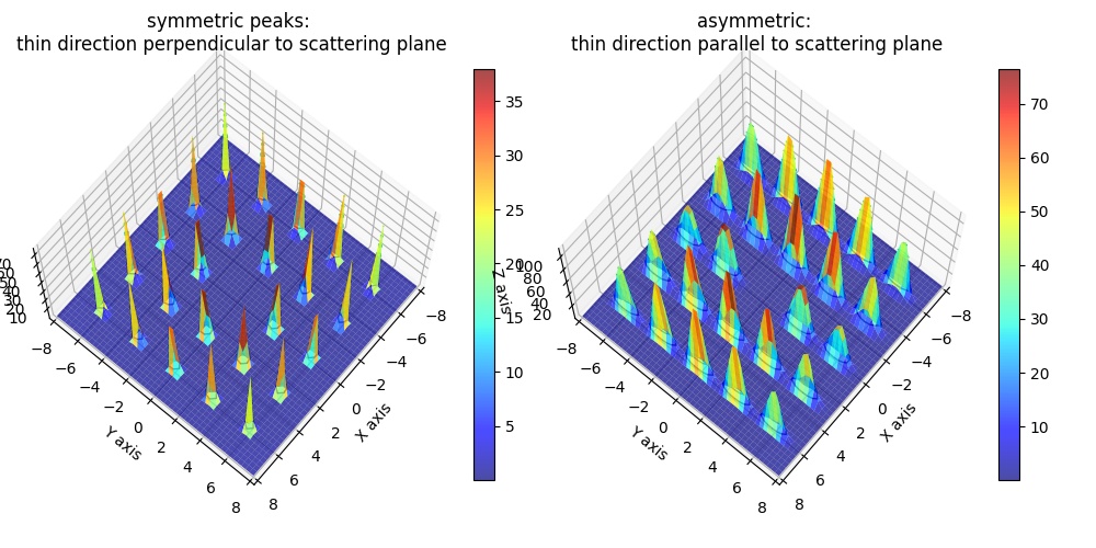
Rotation along axis [1,1,1] leading to broadened peaks. It looks spiky because of low number of points in xy plane. To improve this the user can use more points, which needs longer computing time
import jscatter as js
import numpy as np
# make xy grid in q space
R=8    # maximum
N=800  # number of points
ds=15;
qxy=np.mgrid[-R:R:N*1j, -R:R:N*1j].reshape(2,-1).T
qxyz=np.c_[qxy,np.zeros(qxy.shape[0])].T # add z=0 component

# create sc lattice which includes reciprocal lattice vectors and methods to get peak positions
sclattice= js.lattice.scLattice(3.1, 5)
# Orient 111 direction perpendicular to qxy plane
sclattice.rotatehkl2Vector([1,1,1],[0,0,1])

ffs=js.sf.orientedLatticeStructureFactor(qxyz,sclattice, rotation=[1,1,1,np.deg2rad(10)],
                                        domainsize=ds,rmsd=0.1,hklmax=2,nGauss=23)
fig=js.mpl.surface(ffs.X,ffs.Z,ffs.Y)
fig.axes[0].view_init(70,40)
js.mpl.pyplot.draw()
#fig.savefig(js.examples.imagepath+'/orientedlatticeStructureFactor.jpg')
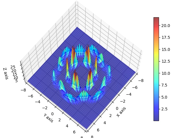
Scattering of a slightly tilted 2D hexagonal plane showing partly the scattering lines in reciprocal space. For 2D planes the Bragg peaks become Bragg lines in reciprocal space that result in elongated scattering patterns when intersecting with the scattering plane. Remember to use the real Ewald sphere. The missing peaks in the x-plane corner are because of hklmax=11.
Homework : try with
rotation = [1,1,1,np.deg2rad(10)]import jscatter as js import numpy as np R=8 # maximum N=200 # number of points ds=40; hex2D_lattice= js.lattice.hex2DLattice(9, 5) hex2D_lattice.rotatehkl2Vector([1,1], [0,60,4]) hex2D_lattice.show() q = np.mgrid[-R:R:200*1j, -R:R:200*1j].reshape(2,-1).T qz=np.c_[q,np.zeros_like(q[:,0])] # for z=0 qy=np.c_[q[:,:1],np.zeros_like(q[:,0]),q[:,1:]] # for z=0 qx=np.c_[np.zeros_like(q[:,0]),q] # for z=0 # rotation = [1,1,1,np.deg2rad(10)] ffz=js.sf.orientedLatticeStructureFactor(qz, hex2D_lattice, rotation=None, domainsize=ds, rmsd=0.1, hklmax=11) ffy=js.sf.orientedLatticeStructureFactor(qy, hex2D_lattice, rotation=None, domainsize=ds, rmsd=0.1, hklmax=11) ffx=js.sf.orientedLatticeStructureFactor(qx, hex2D_lattice, rotation=None, domainsize=ds, rmsd=0.1, hklmax=11) # show as cube surfaces ax=js.mpl.contourOnCube(ffz[[0,1,3]].array,ffx[[1,2,3]].array,ffy[[0,2,3]].array,offset=[-9,-9,9]) ax.set_title('2D hexagonal plane scattering in different directions') #ax.figure.savefig(js.examples.imagepath+'/contour2Dhex.jpg')
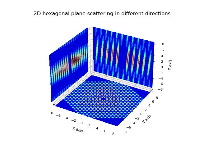
Scattering of a line of scatterers. Now we find scattering planes.
import jscatter as js
import numpy as np
R=8    # maximum
N=200  # number of points
ds=20;

hex2D_lattice= js.lattice.lamLattice(9, 5)
hex2D_lattice.rotatehkl2Vector([1], [0,60,4])
# hex2D_lattice.show()

q = np.mgrid[-R:R:200*1j, -R:R:200*1j].reshape(2,-1).T
qz=np.c_[q,np.zeros_like(q[:,0])]  # for z=0
qy=np.c_[q[:,:1],np.zeros_like(q[:,0]),q[:,1:]]  # for z=0
qx=np.c_[np.zeros_like(q[:,0]),q]  # for z=0

ffz=js.sf.orientedLatticeStructureFactor(qz, hex2D_lattice, domainsize=ds, rmsd=0.1, hklmax=11)
ffy=js.sf.orientedLatticeStructureFactor(qy, hex2D_lattice, domainsize=ds, rmsd=0.1, hklmax=11)
ffx=js.sf.orientedLatticeStructureFactor(qx, hex2D_lattice, domainsize=ds, rmsd=0.1, hklmax=11)

# show as cube surfaces
ax=js.mpl.contourOnCube(ffz[[0,1,3]].array,ffx[[1,2,3]].array,ffy[[0,2,3]].array,offset=[-9,-9,9])
ax.set_title('1D line scattering in different directions')
#ax.figure.savefig(js.examples.imagepath+'/contour1Dlines.jpg')
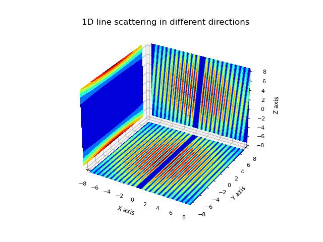
- class jscatter.sf.pseudoRandomLattice(size, numberOfPoints, unitCellAtoms=None, b=None, seed=None)[source]
Bases:
latticeCreate a lattice with a pseudo random distribution of points.
Allows to create 1D, 2D or 3D pseudo random latices. The Halton sequence is used with skipping the first seed elements of the Halton sequence.
- Parameters:
- size :list of 3x float
Size of the lattice for each dimension relative to origin.
- numberOfPointsint
Number of points.
- unitCellAtoms: list of 3x1 array, None=[0,0,0]
Analog to unit cell atoms but distributed around random point. Position vectors vi of atoms in absolute units as random_position+unitCellAtoms[i]. It is not checked if there is an overlap to other atoms.
- bfloat,array
Scattering length of atoms (in unitCellAtoms sequence).
- seedNone, int
Seed for the Halton sequence by skipping the first seed elements of the sequence. If None a random integer between 10 and 1e6 is chosen.
- Returns:
- lattice object
.array grid points as numpy array
Examples
import jscatter as js
grid=js.sf.pseudoRandomLattice([5,5,5],3000)
fig=grid.show()

# three atom basis
grid=js.sf.pseudoRandomLattice([5,5,5],30,unitCellAtoms=[[0,0,0],[0.1,0.1,0],[0.3,0.3,0]],b=[1,2,3])
fig=grid.show()
- jscatter.sf.radial3DLSF(qxyz, lattice=None, domainsize=1000, asym=0, lg=1, rmsd=0.02, beta=None, hklmax=7, c=1.0, wavelength=None, corrections=[])[source]
3D structure factor S(q) in powder average of a crystal lattice with particle asymmetry, DebyeWaller factor, diffusive scattering and broadening due to domain size.
The qxyz can be an arbitrary composition of points in reciprocal space. Uses latticeStructureFactor. The peak shape is a Voigt function.
- Parameters:
- qxyz3xN array
Wavevector plane in inverse units of lattice constant, units 1/A or 1/nm.
- domainsizefloat
Domainsize of the crystal, units as lattice constant of lattice. According to Debye-Scherrer equation \(fwhm=2\pi/domainsize\) the peak width is determined [2].
- latticelattice object
The crystal structure as defined in a lattice object. The size of the lattice is ignored. One of rhombicLattice, bravaisLattice, scLattice, bccLattice, fccLattice, diamondLattice, hexLattice, hcpLattice. See respective definitions.
- lgfloat, default = 1
Lorenzian/gaussian fraction describes the contributions of gaussian and lorenzian shape in peak shape.
lorenzian/gaussian >> 1 lorenzian,
lorenzian/gaussian ~ 1 central part gaussian, outside lorenzian wings
lorenzian/gaussian << 1 gaussian
- asymfloat, default=0
Asymmetry factor in sigmoidal as \(2fwhm/(1+e^{asym*(x-center)})\) For asym=0 the Voigt is symmetric with fwhm. See formel.voigt .
- rmsdfloat, default=0.02
Root mean square displacement \(rmsd=<u^2>^{0.5}\) determining the Debye Waller factor. Units as domainsize and lattice units. Here Debye Waller factor is used as \(DW(q)=e^{-q^2 rmsd^2 }\)
- betafloat, None, dataArray
Asymmetry factor of the formfactor or reduction due to polydispersity.
None beta=1, No beta assumed (spherical symmetric formfactor, no polydispersity)
dataArray explicitly given as dataArray with beta in .Y column. Missing values are interpolated.
An approximation for polydisperse beta can be found in [1] equ.17. This can be realized by beta=js.dA(np.vstack(q,np.exp(-(q*sr*R)**2))) with sr as relative standard deviation of gaussian distribution of the size R.
See .formfactor for different formfactors which explicit calculation of beta.
- hklmaxint
Maximum order of the Bragg peaks to include.
- cfloat, default=1
Porod constant. See 3.8 in [1].
- wavelengthfloat, default = None
Wavelength of the measurement in units nm. If None .Braggtheta is not calculated. For Xray Cu K_a it is 0.15406 nm.
- correctionslist, default=[]
List of corrections to apply, which depend on the measurement type/geometry. See
latticeStructureFactor()
- Returns:
- dataArray
Columns [qx,qz,qw,Sq]
Sq = S(q) = 1+beta(q)*(Z0(q)-1)*DW(q) structure factor
Attributes
.q_hkl peak positions
.fhkl symmetry factor
.mhkl multiplicity
Notes
See latticeStructureFactor.
References
[1] (1,2)Scattering curves of ordered mesoscopic materials. Förster, S. et al. J. Phys. Chem. B 109, 1347–1360 (2005).
[2]Patterson, A. The Scherrer Formula for X-Ray Particle Size Determination Phys. Rev. 56 (10): 978–982 (1939) doi:10.1103/PhysRev.56.978.
[3]Kotlarchyk and S.-H. Chen, J. Chem. Phys. 79, 2461 (1983).1
Examples
import jscatter as js
import numpy as np
import matplotlib.pyplot as pyplot
from matplotlib import cm
from matplotlib import colors
norm=colors.LogNorm(clip=True)

# create lattice
sclattice = js.lattice.scLattice(2.1, 1)
ds = 50

# add flat detector xy plane
xzw = np.mgrid[-8:8:500j, -8:8:500j]

qxzw = np.stack([np.zeros_like(xzw[0]), xzw[0], xzw[1]], axis=0)
ff1 = js.sf.radial3DLSF(qxzw.reshape(3, -1).T, sclattice, domainsize=ds, rmsd=0.03, hklmax=7)
norm.autoscale(ff1.Y)
fig = pyplot.figure()
ax = fig.add_subplot(1, 1, 1)
im = ax.imshow(ff1.Y.reshape(500,-1),norm=norm)
fig.colorbar(im, shrink=0.8)
js.mpl.show()
Note that for to low number of points in the xzw plane Moiré patterns appear.
import jscatter as js
import numpy as np

import matplotlib.pyplot as pyplot
from matplotlib import cm

# Set the aspect ratio to 1 so our sphere looks spherical
fig = pyplot.figure(figsize=pyplot.figaspect(1.))
ax = fig.add_subplot(111, projection='3d')

# create lattice
sclattice = js.lattice.scLattice(2.1, 1)
ds = 50

# add flat detector xy plane
xzw = np.mgrid[-8:8:250j, -8:8:250j]

qxzw = np.stack([np.zeros_like(xzw[0]), xzw[0], xzw[1]], axis=0)
ff1 = js.sf.radial3DLSF(qxzw.reshape(3, -1).T, sclattice, domainsize=ds, rmsd=0.03, hklmax=7)
ffs1 = ff1.Y # np.log(ff1.Y)
fmax, fmin = ffs1.max(), ffs1.min()
ff1Y = (np.reshape(ffs1, xzw[0].shape) - fmin) / (fmax - fmin)
ax.plot_surface(qxzw[0], qxzw[1], qxzw[2], rstride=1, cstride=1, facecolors=cm.gist_ncar(ff1Y), alpha=0.3)

qxzw = np.stack([xzw[0]+8, np.zeros_like(xzw[0])+8,  xzw[1]], axis=0)
ff2 = js.sf.radial3DLSF(qxzw.reshape(3, -1).T, sclattice, domainsize=ds, rmsd=0.03, hklmax=7)
ffs2 = ff2.Y #np.log(ff2.Y)
fmax, fmin = ffs2.max(), ffs2.min()
ff2Y = (np.reshape(ffs2, xzw[0].shape) - fmin) / (fmax - fmin)
ax.plot_surface(qxzw[0], qxzw[1], qxzw[2], rstride=1, cstride=1, facecolors=cm.gray(ff2Y), alpha=0.3)

ax.set_xlabel('x axis')
ax.set_ylabel('y axis')
ax.set_zlabel('z axis')
fig.suptitle('Scattering planes of simple cubic lattice \nin powder average')
pyplot.show(block=False)
- jscatter.sf.radialorientedLSF(*args, **kwargs)[source]
Radial averaged structure factor S(q) of an oriented crystal lattice calculated as orientedLatticeStructureFactor.
For a detailed description and parameters see orientedLatticeStructureFactor. Additionally the qxyz plane according to orientedLatticeStructureFactor is radial averaged over qxyz.
- Parameters:
- qint, array
Explicit list of q values or number of points between min and max wavevector values To large number results in noisy data as the average gets artificial. Each q points will be averaged in intervals around q neighbors from values in qxyz plane.
- Returns:
- dataArray
Columns [q,Sq,DW,beta,Z0q]
q wavevector as norm(qx,qy,qz)
Sq = S(q) = 1+beta(q)*(Z0(q)-1)*DW(q) structure factor
DW(q) Debye-Waller factor with (1-DW)=diffusive scattering.
beta(q) asymmetry factor of the formfactor.
Z0q lattice factor Z0(q)
Attributes (+ input parameters)
.q_hkl peak positions
.hkl Miller indices
.peakFWHM full width half maximum
Notes
qxyz might be any number and geometrical distribution as plane or 3D cube. 3D qxyz points will be converted to qr=norm(qxyz) and averaged.
Examples
import jscatter as js
import numpy as np

R=12
N=200
ds=10
fcclattice= js.lattice.fccLattice(3.1, 5)
qxy=np.mgrid[-R:R:N*1j, -R:R:N*1j].reshape(2,-1).T
qxyz=np.c_[qxy,np.zeros(N**2)].T
q=np.r_[0.1:16:100j]
p=js.grace()
for rmsd in [0.07,0.03,0.01]:
    ffe=js.sf.radialorientedLSF(q=q,qxyz=qxyz,lattice=fcclattice,rotation=[1,1,1,np.deg2rad(10)],domainsize=ds,rmsd=rmsd,hklmax=6)
    p.plot(ffe,li=1,le=f'rmsd {rmsd}')
p.legend(x=8,y=1.8)
p.yaxis(label='S(Q)',min=0,max=2.2)
p.xaxis(label='Q / nm\S-1')
#p.save(js.examples.imagepath+'/radialorientedLSF.jpg')
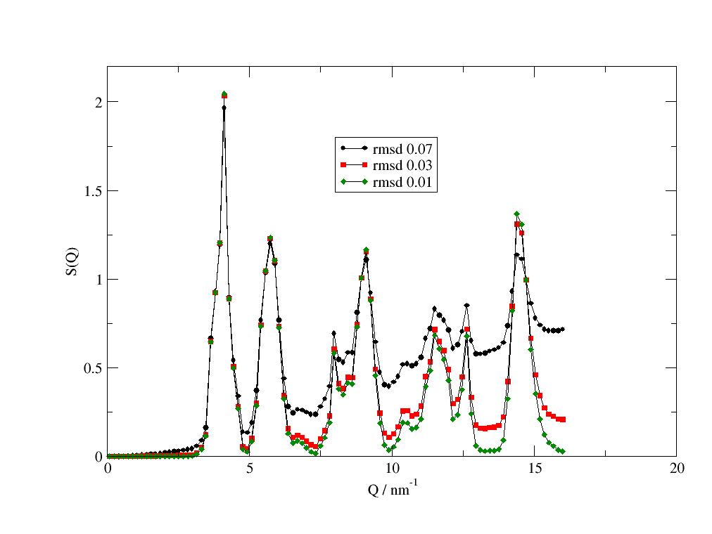
- class jscatter.sf.randomLattice(size, numberOfPoints, b=None, seed=None)[source]
Bases:
latticeCreate a lattice with a random distribution of points.
Allows to create 1D, 2D or 3D random lattices. Uses numpy.random.random.
- Parameters:
- size :3x float
Size of the lattice for each dimension relative to origin.
- numberOfPointsint
Number of points.
- bfloat,array
Scattering length of atoms. If array the sequence is repeated to fill N atoms.
- seedNone, int
Seed for random.
- Returns:
- lattice object
.array grid points as numpy array
Examples
import jscatter as js
grid=js.sf.randomLattice([5,5,5],3000)
fig=grid.show()
- class jscatter.sf.rhombicLattice(latticeVectors, size, unitCellAtoms=None, b=None)[source]
Bases:
latticeCreate a rhombic lattice with specified unit cell atoms which can also represent lattices of mesoscopic particles.
Allows to create 1D, 2D or 3D latices by using 1, 2 or 3 latticeVectors. This can generate classical Bravais lattices but the unit cell atom may also build a coarse grained complex particle like a cylinder or ellipsoid. In
latticeStructureFactor()the particle formfactor amplitude is taken into account.- Parameters:
- latticeVectorslist of array 3x1
Lattice vectors defining the translation of the unit cell along its principal axes.
- size :list of integer
A list of integers describing the size in direction of the respective latticeVectors. Size is symmetric around zero in interval [-i,..,i] with length 2i+1.
- unitCellAtomslist of 3x1 array, None=[0,0,0]
Position vectors vi of atoms in the unit cell in relative units of the lattice vectors [0<x<1]. For 2D and 1D the unit cell atoms vectors are len(vi)=2 and len(vi)=1.
- blist of float
Corresponding scattering length of atoms in the unit cell.
- Returns:
- lattice object
.array : grid points as numpy array
.unitCellVolume : V = a1*a2 x a3 with latticeVectors a1, a2, a3; if existing.
.dim : dimensionality
.unitCellAtoms : Unit cell atoms in relative coordinates
.unitCellAtoms_b : Scattering length of specific unit cell atoms
Examples
A diatomic base
import jscatter as js
grid=js.sf.rhombicLattice(latticeVectors=[[1,0,0],[0,1,0],[0,0,1]],
                           size=[3,3,3],
                           unitCellAtoms=[[-0.1,-0.1,-0.1],[0.1,0.1,0.1]],
                           b=[1,2])
grid.show(1.5)
A cylinder in a hexagonal lattice
import jscatter as js
import numpy as np

# create lattice vectors in a simple way
hex = js.sf.hexLattice(4,8,1)

# create cylinder with atoms in much shorter distance than hex lattice
cylinder = js.sf.scLattice(0.3,[6,6,13])
cylinder.move([0,0,3])
cylinder.inCylinder(v=[0,0,1], R=0.8, a=[0,0,0.5], length=6, b=0, invert=True)

# Convert the cylinder points coordinates to
# fractional unit cell coordinates of the hexagonal lattice
mat = np.linalg.inv(hex.latticeVectors).T
cellAtoms = mat @ cylinder.XYZ.T

grid=js.sf.rhombicLattice(latticeVectors=hex.latticeVectors,
                           size=[1,1,1],
                           unitCellAtoms=cellAtoms.T,
                           b=cylinder.b)
fig = grid.show()
# fig.savefig(js.examples.imagepath+'/grid_hexlyotropic.jpg')
- getRadialReciprocalLattice(size)[source]
Get radial distribution of Bragg peaks with unit cell structure factor and multiplicity.
To get real Bragg peak intensities the dimension in lattice directions has to be included (+ Debye-Waller factor and diffusive scattering). Use latticeStructureFactor to include these effects.
- Parameters:
- sizeint
Size of the lattice as maximum included Miller indices.
- Returns:
- list of [unique q values, structure factor fhkl(q)**2, multiplicity mhkl(q), hkl indices]
Notes
The list contains distinct reflections. If multiplicities are different than expected, e.g. 18 for hex2D the reason is that peaks are degenerate as hk {35} and {70} result in the same Q adding up the multiplicity 18=6+12 . In the radial reciprocal lattice these cannot be separated.
- getReciprocalLattice(size=2, threshold=0.001)[source]
Reciprocal lattice of given size with peak scattering intensity.
- Parameters:
- size3x int or int, default 2
Number of reciprocal lattice points in each direction (+- direction).
- thresholdfloat
Threshold for selection rule as select if (f2_hkl > max(f2_hkl)*threshold)
- Returns:
- Array [N x 7] with
reciprocal lattice vectors [:,:3] corresponding structure factor fhkl**2>0 [:, 3] corresponding indices hkl [:,4:]
Notes
The threshold for selection rules allows to exclude forbidden peaks but include these for unit cells with not equal scattering length as in these cases the selection rule not applies to full extend. This is prefered over a explicit list of selection rules.
- getScatteringAngle(wavelength=None, size=13)[source]
Get scattering angle \(\theta=2arcsin(q_{hkl}\lambda/4\pi)\) in degrees.
- Parameters:
- wavelengthfloat, 0.15406
Wavelength \(\lambda\) in unit nm, default is Cu K-alpha 0.15406 nm.
- sizeint
Maximum size of reciprocal lattice.
- Returns:
- array in degrees
- isRhombic = True
- rotateAroundhkl(hkl, angle=None, vector=None, hkl2=None)[source]
Rotate lattice around hkl direction by angle or to align to vector.
Uses angle or aligns hkl2 to vector. Includes rotation of latticeVectors.
- Parameters:
- hkl3x float
Direction given as Miller indices.
- anglefloat
Rotation angle in rad.
- vector3x float
Vector to align hkl2 to. Overrides angle. Should not be parallel to hkl direction.
- hkl23x float
Direction to align along vector. Overrides angle. Should not be parallel to hkl direction.
Examples
import jscatter as js
import numpy as np
R=8
N=10
qxy=np.mgrid[-R:R:N*1j, -R:R:N*1j].reshape(2,-1).T
qxyz=np.c_[qxy,np.zeros(N**2)]
fccgrid = js.lattice.fccLattice(2.1, 1)
fig=js.mpl.figure( )
# create subplot to define geometry
fig.add_subplot(2,2,1,projection='3d')
fccgrid.show(fig=fig,ax=1)
fccgrid.rotatehkl2Vector([1,1,1],[1,0,0])
fccgrid.show(fig=fig,ax=2)
fccgrid.rotateAroundhkl([1,1,1],np.deg2rad(30))
fccgrid.show(fig=fig,ax=3)
fccgrid.rotateAroundhkl([1,1,1],[1,0,0],[1,0,0])
fccgrid.show(fig=fig,ax=4)
- rotatePlane2hkl(plane, hkl, basis=None)[source]
Rotate plane points that plane is perpendicular to hkl direction.
- Parameters:
- planearray Nx3
3D points of plane to rotate. If None the rotation matrix is returned.
- hkllist of int, float
Miller indices as [1,1,1] indicating the lattice direction where to rotate to.
- basisarray min 3x3, default=None
3 basis points spanning the plane to define rotation. e.g.[[0,0,0],[1,0,0],[0,1,0]] for xy plane. If None the first points of the plane are used instead.
- Returns:
- rotated plane points array 3xN
- or rotation matrix 3x3
Notes
The rotation matrix may be used to rotate the plane to the desired direction.
R = grid.rotatePlane2hkl(None,[1,1,1],[[0,0,0],[1,0,0],[0,1,0]] )
newplanepoints = np.einsum('ij,kj->ki', R, planepoints)
or the transposed R can be used to rotate the lattice.
R = grid.rotatePlane2hkl(None,[1,1,1],[[0,0,0],[1,0,0],[0,1,0]] )
grid.rotatebyMatrix(R.T)
Examples
import jscatter as js
import numpy as np
R=8
N=10
qxy=np.mgrid[-R:R:N*1j, -R:R:N*1j].reshape(2,-1).T
qxyz=np.c_[qxy,np.zeros(N**2)]
fccgrid = js.lattice.fccLattice(2.1, 2)
xyz=fccgrid.rotatePlane2hkl(qxyz,[1,1,1])

p=js.mpl.scatter3d(xyz[:,0],xyz[:,1],xyz[:,2])
p.axes[0].scatter(fccgrid.X,fccgrid.Y,fccgrid.Z)
- rotatePlaneAroundhkl(plane, hkl, angle)[source]
Rotate plane points around hkl direction.
- Parameters:
- planearray Nx3, None
3D points of plane. If None the rotation matrix is returned.
- hkllist of int, float
Miller indices as [1,1,1] indicating the lattice direction to rotate around.
- anglefloat
Angle in rad
- Returns:
- plane points array 3xN
- or rotation matrix
Notes
The rotation matrix may be used to rotate the plane to the desired direction.
R = grid.rotatePlaneAroundhkl(None,[1,1,1],1.234)
newplanepoints = np.einsum('ij,kj->ki', R, planepoints)
or the transposed R can be used to rotate the lattice.
grid.rotatebyMatrix(R.T)
Examples
import jscatter as js
import numpy as np
R=8
N=10
qxy=np.mgrid[-R:R:N*1j, -R:R:N*1j].reshape(2,-1).T
qxyz=np.c_[qxy,np.zeros(N**2)]
fccgrid = js.lattice.fccLattice(2.1, 1)
xyz=fccgrid.rotatePlane2hkl(qxyz,[1,1,1])
xyz2=fccgrid.rotatePlaneAroundhkl(xyz,[1,1,1],np.deg2rad(30))
p=js.mpl.scatter3d(xyz[:,0],xyz[:,1],xyz[:,2])
p.axes[0].scatter(xyz2[:,0],xyz2[:,1],xyz2[:,2])
p.axes[0].scatter(fccgrid.X,fccgrid.Y,fccgrid.Z)
- rotatebyMatrix(R)[source]
Rotate lattice by rotation matrix including reciprocal vectors (in place).
- Parameters:
- R3x3 array
Rotation matrix.
- rotatehkl2Vector(hkl, vector)[source]
Rotate lattice that hkl direction is parallel to vector.
Includes rotation of latticeVectors.
- Parameters:
- hkl3x float
Direction given as Miller indices.
- vector3x float
Direction to align to.
Examples
import jscatter as js
import numpy as np
R=8
N=10
qxy=np.mgrid[-R:R:N*1j, -R:R:N*1j].reshape(2,-1).T
qxyz=np.c_[qxy,np.zeros(N**2)]

fccgrid = js.lattice.fccLattice(2.1, 1)
p=js.mpl.scatter3d(fccgrid.X,fccgrid.Y,fccgrid.Z)

fccgrid.rotatehkl2Vector([1,1,1],[1,0,0])
p.axes[0].scatter(fccgrid.X,fccgrid.Y,fccgrid.Z)

fccgrid.rotateAroundhkl([1,1,1],np.deg2rad(30))
p.axes[0].scatter(fccgrid.X,fccgrid.Y,fccgrid.Z)
- property unitCellAtomPositions
Absolute positions of unit cell atoms.
- class jscatter.sf.scLattice(abc, size, b=None)[source]
Bases:
bravaisLatticeSimple Cubic lattice.
See rhombicLattice for methods.
- Parameters:
- abcfloat
Lattice constant of unit cell.
- size3x integer, integer
A list of integers describing the size in direction of the respective latticeVectors. Size is symmetric around zero in interval [-i,..,i] with length 2i+1. If one integer is given it is used for all 3 dimensions.
- blist of float
Corresponding scattering length of atoms in the unit cell.
- Returns:
- lattice object
.array grid points as numpy array
Examples
import jscatter as js
grid=js.sf.bccLattice(1.2,1)
grid.show(2)
- jscatter.sf.sq2gr(Sq, R, interpolatefactor=2)[source]
Radial distribution function g(r) from structure factor S(Q).
The result strongly depends on quality of S(Q) (number of data points, Q range, smoothness). Read [2] for details of this inversion problem and why it may fail.
After a fit of S(Q) to exp. data a simulated S(Q) with extended Q range may be used to get g(r).
- Parameters:
- SqdataArray
Structure factor to transform
.X wavevector in units as [Q]=1/nm
.Y structure factor
Advice : Use more than \(2^{10}\) points and \(Q_{max}R>\) for accurate results.
Sq is internally interpolated by a cubic spline to get equidistant points.
- Rfloat
Estimate for the radius of the particles. Used for requirement \(mean(g(R/2<r<R 3/4)) = 0\)
- interpolatefactorint
Number of additional points between Sq points to interpolate. 2 doubles the existing points.
- Returns:
- g(r)dataArray
.n0 approximated from \(2\pi^2 n_0=\int_0^{Q_{max}} [S(Q) -1]Q^2 dQ\)
Notes
One finds that ([1] equ. 7)
\[g(r)-1=(2\pi^2 n_0 r)^{-1} \int_0^\infty [S(Q) -1]Qsin(qr)dQ\]and ([1] equ. 6)
\[S(q)-1 = (4\pi^2 n_0 / q) \int_0^\infty [g(r) -1]rsin(qr)dr\]with defining \(n_0\) and \(S(0)\)
\[2\pi^2 n_0=\int_0^\infty [S(Q) -1]Q^2 dQ\]\[S(0) = 1 + 4\pi^2 n_0 \int_V [g(r) -1] d\vec{r}\]As we have only a limited Q range (\(0 < Q < \infty\) ), limited accuracy and number of Q values we require that \(mean(g(R/2<r<R3/4))=0\).
References
[1] (1,2)Yarnell, J. L., Katz, M. J., Wenzel, R. G., & Koenig, S. H. (1973). Structure factor and radial distribution function for liquid argon at 85 K. Physical Review A, 7(6), 2130.
[2]On the determination of the pair correlation function from liquid structure factor measurements A.K. Soper Chemical Physics 107, 61-74, (1986)
Examples
The example shows that a Percus-Yevick like hard sphere structure factor (RMSA with small gamma) has a high probability that the cores are close to 2R. This is reduced if a reasonable repulsion is present.
import jscatter as js
import numpy as np
p=js.grace()
p.multi(2,1)
q=np.r_[0.001:30:1j*2**10]
p[0].clear();p[1].clear()
R=2.5
eta=0.3;scl=5
n=eta/(4/3.*np.pi*R**3)   # unit 1/nm**3
sf=js.sf.RMSA(q=q,R=R,scl=scl, gamma=50, eta=eta)
gr=js.sf.sq2gr(sf,R,interpolatefactor=1)

# same with Qmax=10
sfcut=js.sf.RMSA(js.loglist(0.01,10,2**10),R=R,scl=scl, gamma=50, eta=eta)
grcut=js.sf.sq2gr(sfcut,R,interpolatefactor=5)

p[0].plot(sf.X*2*R,sf.Y,le=r'\xG=50')
p[1].plot(gr.X/2/R,gr[1],le=r'\xG=50')
p[1].plot(grcut.X/2/R,grcut[1],le=r'\xG=50 \f{}Q\smax\N=10')

# a small gamma like a hard sphere potential
sfh=js.sf.RMSA(q=q,R=R,scl=scl, gamma=0.01, eta=eta)
grh=js.sf.sq2gr(sfh,R,interpolatefactor=1)
p[0].plot(sfh.X*2*R,sfh.Y,le=r'\xG=0.01')
p[1].plot(grh.X/2/R,grh[1],le=r'\xG=0.01')

p[0].xaxis(max=20,label='2RQ')
p[1].xaxis(max=4*R,label='r/(2R)')
p[0].yaxis(max=2,min=0,label='S(Q)')
p[1].yaxis(max=2.5,min=0,label='g(r)')
p[0].legend(x=10,y=1.8)
p[1].legend(x=4,y=2.2)
p[0].title('Comparison RMSA')
p[0].subtitle('R=%.2g, eta=%.2g, scl=%.2g' %(R,eta,scl))
#p.save(js.examples.imagepath+'/sq2gr.jpg')
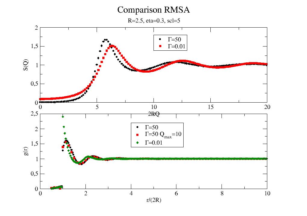
- class jscatter.sf.sqLattice(ab, size, b=None)[source]
Bases:
bravaisLatticeSimple 2D square lattice.
See rhombicLattice for methods.
- Parameters:
- abfloat
Lattice constant of unit cell.
- size2x integer, integer
A list of integers describing the size in direction of the respective latticeVectors. Size is symmetric around zero in interval [-i,..,i] with length 2i+1. If one integer is given it is used for all 3 dimensions.
- blist of float
Corresponding scattering length of atoms in the unit cell.
- Returns:
- lattice object
.array grid points as numpy array
Examples
import jscatter as js
grid=js.sf.sqLattice(1.2,1)
grid.show(2)
- jscatter.sf.stickyHardSphere(q, R, width, depth, molarity=None, phi=None)[source]
Structure factor of a square well potential with depth and width (sticky hard spheres).
Sticky hard sphere model is derived using a perturbative solution of the factorized form of the Ornstein-Zernike equation and the Percus-Yevick closure relation.
The perturbation parameter is width/(width+2R) S(Q) is defined in [1] equation 29 .
- Parameters:
- qarray; N dim
Scattering vector; units 1/(R[unit])
- Rfloat
Radius of the hard sphere
- phifloat
Volume fraction of the hard core particles
- molarityfloat
Number density in mol/l and defines q and R units to 1/nm and nm to be correct Preferred over phi if both given.
- depthfloat
Potential well depth in kT depth >0 (U<0); positive potential allowed (repulsive) see [1].
- widthfloat
Width of the square well
- Returns:
- S(Q)dataArray
Notes
The potential U(r) is defined as
\[\begin{split}\begin{align} U(r) &= \infty & r<2R \\ &= -depth[kT] & 2R<r<2R+width \\ &= 0 & r>2R+width \end{align}\end{split}\]Other definitions include
eps=width/(2*R+width)
stickiness=exp(-depth)/12./eps
References
[2]Sztucki, T. Narayanan, G. Belina, A. Moussaïd, F. Pignon, and H. Hoekstra, Phys. Rev. E 74, 051504 (2006)
[3]W.-R. Chen, S.-H. Chen, and F. Mallamace, Phys. Rev. E 66, 021403 (2002)
[4]Foffi, E. Zaccarelli, F. Sciortino, P. Tartaglia, and K. A. Dawson, J. Stat. Phys. 100, 363 (2000)
Examples
import jscatter as js
R = 6
phi = 0.05
depth = 15
q = js.loglist(0.01, 2, 200)
p = js.grace(1,1)
for eta in [0.005,0.01,0.03,0.05,0.1,0.2]:
    shs = js.sf.stickyHardSphere(q, R, 1, 3, phi=eta)
    p.plot(shs, symbol=0, line=[1, 3, -1], legend=f'eta ={eta:.3f}')
p.yaxis(min=0.0, max=3.2, label='S(Q)', charsize=1.5)
p.legend(x=1, y=3)
p.xaxis(min=0, max=1.5)
p.title('sticky hard sphere structure factor')
#p.save(js.examples.imagepath+'/stickyHardSphere.jpg')
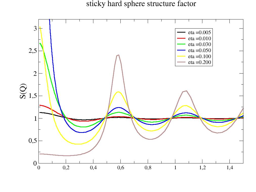
- jscatter.sf.twoYukawa(q, R, K1, K2, scl1, scl2, molarity=None, phi=None)[source]
Structure factor for a two Yukawa potential in mean spherical approximation.
A two Yukawa potential in the mean spherical approximation describing cluster formation in the two-Yukawa fluid when the interparticle potential is composed of a short-range attraction and a long-range repulsion according to Liu et al.[R76bf1e2cc48d-1]_.
- Parameters:
- qarray
Wavevectors in units 1/nm.
- K1,K2float
Potential strength in units kT.
K>0 attraction
K<0 repulsion
- scl1,scl2float
Screening length in units nm. The inverse screening length is \(Z_i=1/scl_i\).
- Rfloat
Radius of the particle in nm.
- phifloat
Volume fraction of particles in the solution.
- molarityfloat
concentration in units mol/l. Overrides phi if both given.
- Returns:
- dataArray[q,Sq]
additional input attributes
On errors in calculation Sq=0 is returned to prevent errors during fitting. These are no physical solution.
Notes
The reduced potential (with \(Z_i=1/scl_i\) and r scaled to yield a hardcore diameter of 1) is:
\[ \begin{align}\begin{aligned}\frac{V(r)}{kT} &= \infty \; &for \; 0<r<1\\&= -K_1 \frac{e^{-Z_1 (r-1)}}{r} -K_2 \frac{e^{-Z_2 (r-1)}}{r} \; &for \; r>1\end{aligned}\end{align} \]within the MSA closure
\[ \begin{align}\begin{aligned}h(r) &=-1 \; &for \; 0<r<1\\c(r) &= -\frac{V(r)}{kT} \; &for \; r>1\end{aligned}\end{align} \]Internally, Z1>Z2 (=> scl1<scl2) is forced, which is accompanied in the Python code by a swap of K1<>K2 that fitting is smoother.
For unphysical or no solution zero is returned.
The solution is unstable close to Z1=Z2. In these cass the (R)MSA structure factor (single Yukawa) is more appropriate. The function tries to approximate a solution using K2=>(K1+K2), K1=>0.001K2,Z1=2 Z2
About the code: This Python version of TwoYukawa is based on the code from the IGOR version taken from NCNR_SANS_package by Steve Kline (https://github.com/sansigormacros/ncnrsansigormacros) The Igor version of this function is based in part on Matlab code supplied by Yun Liu. The XOP version of this function is based in part on c-code supplied by Marcus Henning.
Please cite the paper [1], if you use the results produced by this code.
References
[1] (1,2)Cluster formation in two-Yukawa fluids Yun Liu, Wei-Ren Chen, and Sow-Hsin Chen THE JOURNAL OF CHEMICAL PHYSICS 122, 044507 (2005) http://dx.doi.org/10.1063/1.1830433
Examples
This reproduces figure 1 in [1]. This figure illustrates the existence of a cluster peak in the structure factor for increasing strength K1 of the long-range attraction.
import numpy as np
import jscatter as js
q = np.r_[0.01:20:300j]
R = 0.5
K2 = -1
scl1 = 1/10
scl2 = 1/0.5
phi =0.2
#
p=js.grace(1,0.7)
for K1 in np.r_[0,3,6,10]:
    Sq = js.sf.twoYukawa(q, R, K1, K2, scl1, scl2, phi=phi)
    p.plot(Sq,li=[1,4,-1],sy=0,le=f'K1={K1:.0f}')
p.xaxis(label='QD',charsize=2)
p.yaxis(label='S(Q)',charsize=2)
p.legend(y=1.95,x=16,charsize=2)
p.subtitle('S(q) of Two-Yukawa Potential',size=2)
p.text(r'cluster \npeak',x=2,y=1.9,charsize=2)
#p.save(js.examples.imagepath+'/twoYukawa.jpg')
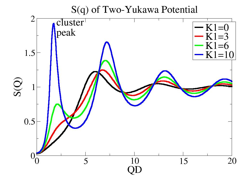
- jscatter.sf.weakPolyelectrolyte(q, cp, l, f, cs, ioc=None, eps=None, Temp=293.15, contrast=None, molarVolume=None)[source]
Monomer-monomer structure factor S(q) of a weak polyelectrolyte according to Borue and Erukhimovich [3].
Polyelectrolyte models based on [3] are valid above “the critical concentration when electrostatic blobs begin to overlap”, see equ. 2 in [3] and above where we don’t see isolated chains. The used RPA is valid only at high polymer concentrations where concentration fluctuations are weak [4].
- Parameters:
- qarray
Scattering vector in units 1/nm.
- cpfloat
Monomer concentration \(c_p\) in units mol/l. The monomer concentration is :math:`N c_{p}.
- lfloat
Monomer length in units nm.
- ffloat
Fraction of charged monomers \(f\). The abs(f) values is used.
- csfloat
Monovalent salt concentration \(c_s\) in the solvent in units mol/l. This may include ions from water dissociation.
- iocfloat, default 0
Additional contribution to the inverse osmotic compressibility Dm of neutral polymer solution in units \(nm^3\). Inverse osmotic compressibility is \(Dm=1/(Nc)+v+w^2c\) (see [2]) The additional contribution is \(ioc=v+w^2c\) as used in [1] and can be positive or negative. \(v\) and \(w\) are the second and third virial coefficients [1].
- epsfloat
Dielectric constant of the solvent to determine the Bjerum length. Default is H2O at given temperature. Use formel.dielectricConstant to determine the constant for your water based solvent including salt. For H2O at 293.15 K = 80.08 . Added 1M NaCl = 91.08
- Tempfloat, default 273.15+20
Temperature in units Kelvin.
- contrastfloat, default None
Contrast of the polymer \(\rho_{monomer}\) relative to the solvent as difference of scattering length densities in units \(nm^{-2}\). See Notes for determination of absolute scattering. contrast and molarVolume need to be given.
- molarVolumefloat, default None
Molar volume \(V_{monomer}\) of the polymer in \(nm^{3}\). See Notes for determination of absolute scattering. contrast and molarVolume need to be given.
- Returns:
- dataArray2 x N
Columns [q, Sq]
.epsilon
.kappa in 1/nm
.screeninglength in nm
.r0 characteristic screening length without salt in units nm.
.c_monomer Monomer concentration in mol/l
.c_salt Salt concentration in mol/l
.c_ions Ion concentration as \(2c_s + fc_p\) in mol/l
.monomerscatteringlength \(c = V_{monomer}\rho_{monomer}\). If contrast or molarVolume are None then c=1.
Sq units is 1/nm = 1/(1e-7 cm) = 1e7 1/cm. (multiply by 1e7 to get units 1/cm)
Notes
Borue and Erukhimovich [3] describe the polyelectrolyte scattering in reduced variables (see [3] equ 39). Rewriting this equation expressing the reduced variables s and t in terms of \(r_0\) yields :
\[S(q) = c^2 \frac{1}{4\pi l_b f^2} \frac{q^2+\kappa^2}{1+r_0^4(q^2+\kappa^2)(q^2-12hc_p/l^2)}\]with
\(r_0^2 = \frac{l}{f\sqrt{48c_p\pi l_b} }\) characteristic scale of screening without salt
\(c=V_{monomer}\rho_{monomer}\) scattering length monomer.
\(l_b = e^2/4\pi\epsilon kT \approx 0.7 nm\) Bjerum length.
\(\kappa^{-1}=\frac{1}{\sqrt{4\pi l_b (\sum_s{2c_s} + fc_p)}}\) Debye-Hückel screening length from salt ions and polymer.
\(h=ioc\) Additional contribution to inverse compressibility.
\(v\) and \(w\) are the second and third virial coefficients between monomers \(\rightarrow ioc=v+w^2c\) [1].
For low salt concentration (\(\kappa < r_0\)) the peak is expected at \((q^{*2}+\kappa^2)^2 = r_0^{-4}\) (see [1] and [2] after euq. 14) and vanishes for \(\kappa > r_0\) (see [2]).
References
[1] (1,2,3,4)Annealed and quenched polyelectrolytes. Raphael, E., & Joanny, J. F. (1990). EPL, 13(7), 623–628. https://doi.org/10.1209/0295-5075/13/7/009
[2] (1,2,3)Weakly charged polyelectrolytes in a poor solvent J.F. Joanny, L. Leibler J. Phys. France 51, 545-557 (1990) DOI: 10.1051/jphys:01990005106054500
[3] (1,2,3,4,5,6)A statistical theory of weakly charged polyelectrolytes: fluctuations, equation of state and microphase separation V. Yu. Borue, I. Ya. Erukhimovich, Macromolecules (1988) 21, 11, 3240-3249
[4]50th Anniversary Perspective: A Perspective on Polyelectrolyte Solutions M. Muthukumar Macromolecules201750249528-9560 See p 9537 Pitfall of RPA for Polyelectrolyte solution
Examples
Poly(sodium 4-styrenesulfonate)(PSS-Na) with a bulk density of 0.801 g/mL. Monomer MW = 184 g/mol, monomer length 2 C-C bonds = 2 * 0.15 nm
import jscatter as js
import numpy as np
q=js.loglist(0.01,4,100)

Vm=184/0.801/6.022140857e+23/1e-21  # partial molar volume of the polymer in nm**3
c=0.000698-0.000942 # PSS in H2O for X-ray scattering has negative contrast
p=js.grace(1.2,1)
for i,cp in enumerate([5, 10, 20, 30, 60],1): # conc in g/l
   c17=cp/184 # conc in mol/l
   Sq=js.sf.weakPolyelectrolyte(q=q, l=0.3, cp=c17, f=0.05, cs=0.005,ioc=0,contrast=c,molarVolume=Vm)
   Sq.Y*=1e7  # conversion to 1/cm
   p.plot(Sq,sy=[i,0.4,i],li=0,le='c={0:.3} mg/ml'.format(c17))
   Sqi=js.sf.weakPolyelectrolyte(q=q, l=0.3, cp=c17, f=0.05, cs=0.005,ioc=-0.02,contrast=c,molarVolume=Vm)
   Sqi.Y*=1e7
   p.plot(Sqi,li=[1,1,i],sy=0,le='ioc=-0.02 c={0:.3} mg/ml'.format(c17))

p.yaxis(scale='log',min=Sq.Y.min()/15,max=Sq.Y.max(),label='I(q) / 1/cm')
p.xaxis(scale='log',min=0.01,max=4,label=r'q / nm\S-1')
p.title('A polyelectrolyte at low salt')
p.legend(x=0.02,y=1.5e-1)
#p.save(js.examples.imagepath+'/weakPolyelectrolyte.png')