12. Examples
These examples show how to use Jscatter. Use showExampleList to get a full list
or look in showExampleList().
A general introduction is in Beginners Guide / Help
Most functions descriptions contain an Example sections with more specific examples.
Examples are mainly based on XmGrace for plotting as this is more convenient for interactive inspection of data and used for most of the shown plots.
Matplotlib can be used by setting usempl=True in runExample and showExample
(automatically set if Grace is not present).
With matplotlib the plots are not optimized but still show the possibilities.
Show an updated list of all examples. |
|
|
Opens example in default editor. |
|
Run example by number or name. |
|
Run all examples ( Maybe needs a bit of time ) . |
Try Jscatter Demo in a Jupyter Notebook at ![]() .
.
12.1. In a nutshell
Daily use example to show how short it can be. A key point is that each dataArray has a ‘q’ which is used in the fit model.
Comments are shown in next examples.
# in nutshell without fine tuning of plots

import jscatter as js
import numpy as np

# read data with 16 intermediate scattering functions from NSE measurement of protein diffusion
i5 = js.dL(js.examples.datapath + '/iqt_1hho.dat')

# manipulate data
for dat in i5:
    dat.X = dat.X /1.  # conversion from ps to ns
    dat.q *= 1  # conversion to 1/nm if needed

# define model as simple diffusion with elastic background
diffusion = lambda A, D, t, elastic, wavevector=0: A * np.exp(-wavevector ** 2 * D * t) + elastic

# make ErrPlot to see progress of intermediate steps with residuals (updated all 2s)
i5.makeErrPlot(title='diffusion model residual plot', legpos=[0.2, 0.8])

# fit it
i5.fit(model=diffusion,  # the fit function
       freepar={'D': [0.2, 0.25], 'A': 1},  # fit start values; [..] indicate independent fit parameter
       fixpar={'elastic': 0.0},             # single values indicates common fit parameter
       mapNames={'t': 'X', 'wavevector': 'q'},  # map names of the model to names of data attributes
       condition=lambda a: (a.X > 0.01) & (a.Y > 0.01))  # a condition to include only specific values

# save fit result with errors and covariance matrix
i5.lastfit.savetxt('iqt_proteindiffusion_fit.dat')

# plot it together with lastfit result
p = js.grace()
p.plot(i5, symbol=[-1, 0.4, -1], legend='Q=$q')  # plot as alternating symbols and colors with size 0.4
p.plot(i5.lastfit, symbol=0, line=[1, 1, -1])  # plot a line with alternating colors
p.save('iqt_proteindiffusion_fit.png')

# plot result with error bars
p1 = js.grace(2, 2)  # plot with a defined size
p1.plot(i5.lastfit.wavevector, i5.lastfit.D, i5.lastfit.D_err, symbol=[2, 1, 1, ''], legend='average effective D')
p1.save('Diffusioncoefficients.agr')  # save as XmGrace plot
12.2. Build models
12.2.1. How to build simple models
# How to build simple models
# which are actually not so simple....

import numpy as np
import jscatter as js

# Build models in one line using lambda
# directly calc the values and return only Y values
diffusion = lambda A, D, t, wavevector, elastic=0: A * np.exp(-wavevector ** 2 * D * t) + elastic

# use a model from the libraries
# here Teubner-Strey adding background and power law
# this returns as above only Y values
tbpower = lambda q, B, xi, dd, A, beta, bgr: js.ff.teubnerStrey(q=q, xi=xi, d=dd).Y * B + A * q ** beta + bgr


# The same as above in a function definition
# This should be the preferred way
def diffusion2(A, D, t, elastic, wavevector=0):
    Y = A * np.exp(-wavevector ** 2 * D * t) + elastic
    return Y


# returning dataArray allows additional attributes to be included in the result
# this returns a dataArray with X, Y values and attributes
# and is how Jscatter model return data
def diffusion3(A, D, t, wavevector, elastic=0):
    Y = A * np.exp(-wavevector ** 2 * D * t) + elastic
    result = js.dA(np.c_[t, Y].T)
    result.diffusioncoefficient = D
    result.wavevector = wavevector
    result.columnname = 'time;Iqt'
    return result


# supplement an existing model
def tbpower2(q, B, xi, dd, A, beta, bgr):
    """Model Teubner Strey  + power law and background"""
    # save different contributions for later analysis
    tb = js.ff.teubnerStrey(q=q, xi=xi, d=dd)
    pl = A * q ** beta  # power law
    tb = tb.addZeroColumns(2)
    tb[-2] = pl  # save power law in new last column
    tb[-1] = tb.Y  # save Teubner-Strey in last column
    tb.Y = B * tb.Y + pl + bgr  # put full model to Y values (usually tb[1])
    # save the additional parameters ; xi and d already included in teubnerStrey
    tb.A = A
    tb.bgr = bgr
    tb.beta = beta
    tb.columnname = 'q;Iq,IqTb,Iqpower'
    return tb

# How to add a numpy like docstring see in the example "How to build a complex model".
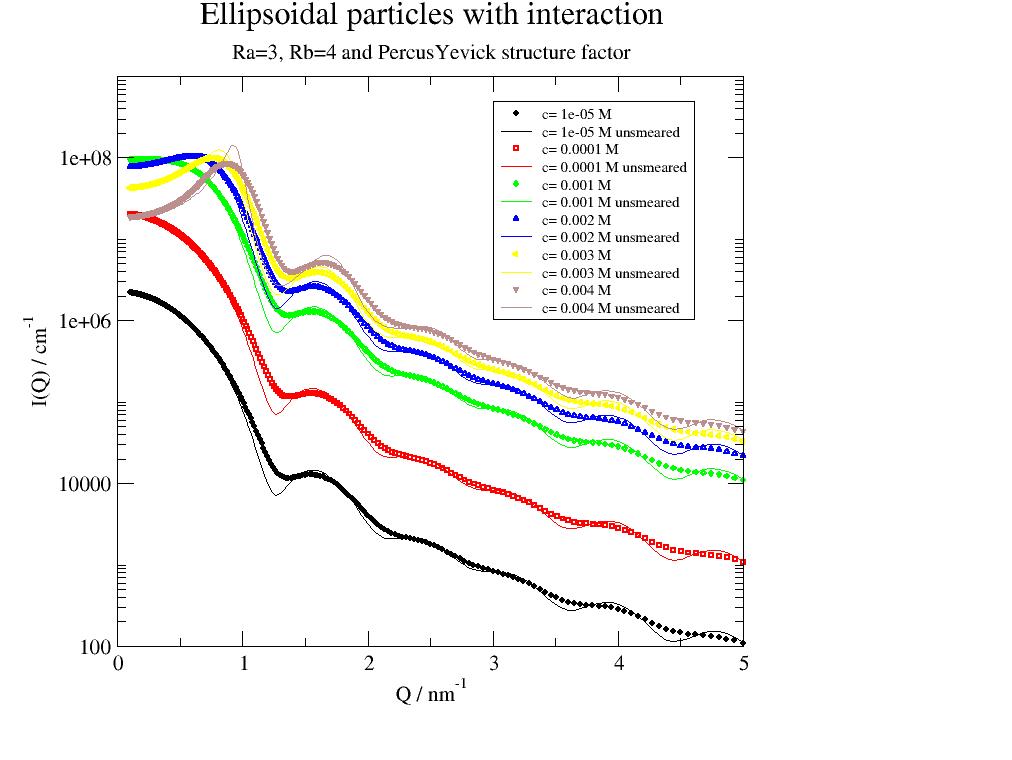
12.2.2. How to build a more complex model
# How to build a complex model

import jscatter as js

resol2m = js.sas.prepareBeamProfile('SANS', detDist=2000, collDist=2000., wavelength=0.7, wavespread=0.10,
                                    collAperture=30, sampleAperture=6, dpixelWidth=10, dringwidth=1)


# build a complex model of different components inclusive smearing
# @js.sas.smear does the smearing of the model in the following line

@js.sas.smear(beamProfile=resol2m)
def particlesWithInteraction(q, Ra, Rb, molarity, bgr, contrast=1, detDist=None, collDist=None, beta=True):
    """
    Particles with interaction and ellipsoid form factor as a model for e.g. dense protein solutions.

    Document your model if needed for later use that you know what you did and why.
    Or make it short without all the nasty documentation for testing.
    The example neglects the protein exact shape and non constant scattering length density.
    Proteins are more potato shaped  and nearly never like a ellipsoid or sphere.
    So this model is only valid at low Q as an approximation.

    Parameters
    ----------
    q : float
        Wavevector
    Ra,Rb : float
        Radius
    molarity : float
        Concentration in mol/l
    contrast : float
        Contrast between ellipsoid and solvent.
    bgr : float
        Background e.g. incoherent scattering
    detDist,collDist : float, None
        detector distance and collimation length for SANS and SAXS.
        If any is None no smearing is used.
        Both need not to be used in the model function.
    beta : bool
        True include asymmetry factor beta of
        M. Kotlarchyk and S.-H. Chen, J. Chem. Phys. 79, 2461 (1983).

    Returns
    -------
        dataArray

    Notes
    -----
    Explicitly:
    **The return value can be a dataArray OR only Y values**. Both is working for fitting.

    **About smearing during a fit with mixed SANS and or SAXS**:

    Data to fit should have attributes with smear parameters as detDist and more .
    For SAXS we set detDist=None (bypass smearing ==no smearing) or we set parameters for SAXS smearing.
    For SANS  we set some reasonable values as 2000 (mm) or 20000 (mm) for detDist and collDist.
    Missing parameters are used from beamProfile as given in the decorator.

    """
    # We need to multiply form factor and structure factor and add an additional background.
    # formfactor of ellipsoid returns dataArray with beta at last column.
    ff = js.ff.ellipsoid(q, Ra, Rb, SLD=contrast)
    V = ff.EllipsoidVolume
    # the structure factor returns also dataArray
    # we need to supply a radius calculated from Ra Rb, this is an assumption of effective radius for the interaction.
    R = (Ra * Rb * Rb) ** (1 / 3.)
    # the volume fraction is concentration * volume
    # the units have to be converted as V is usually nm**3 and concentration is mol/l
    sf = js.sf.PercusYevick(q, R, molarity=molarity)
    if beta:
        # beta is asymmetry factor according to M. Kotlarchyk and S.-H. Chen, J. Chem. Phys. 79, 2461 (1983).
        # correction to apply for the structure factor
        # noinspection PyProtectedMember
        sf.Y = 1 + ff._beta * (sf.Y - 1)
    #
    # molarity (mol/l) with conversion to number/nm**3 result is in cm**-1
    ff.Y = molarity * 6.023e23 / (1000 * 1e7 ** 2) * ff.Y * sf.Y + bgr
    # add parameters for later use; ellipsoid parameters are already included in ff
    # if data are saved these are included in the file as documentation
    # or can be used for further calculations e.g. if volume fraction is needed (V*molarity)
    ff.R = R
    ff.bgr = bgr
    ff.Volume = V
    ff.molarity = molarity

    return ff


p = js.grace()
q = js.loglist(0.1, 5, 300)
for i, m in enumerate([0.01, 0.1, 1, 2, 3, 4], 1):
    data = particlesWithInteraction(q, Ra=3, Rb=4, molarity=m * 1e-3, bgr=0, contrast=1, detDist=2000, collDist=2000)
    p.plot(data, sy=[i, 0.3, i], le='c= $molarity M')
    p.plot(data.X, data[2], sy=0, li=[1, 1, i], le='c= {0:} M unsmeared'.format(data.molarity))

p.legend(x=3, y=5e8, charsize=0.7)
p.yaxis(min=100, max=1e9, scale='l', label=r'I(Q) / cm\S-1', tick=[10, 9])
p.xaxis(scale='n', label=r'Q / nm\S-1')
p.title('Ellipsoidal particles with interaction')
p.subtitle('Ra=3, Rb=4 and PercusYevick structure factor')
# Hint for fitting SANS data or other parameter dependent fit:
# For a combined fit of several collimation distances each dataset should contain an attribute data.collimation.
# This is automatically used in the fit, if there is not explicit fit parameter with this name.

if 1:
    p.save('interactingParticles.agr')
    p.save('interactingParticles.jpeg')
12.3. Fitting 1D, 2D 3D …
12.3.1. 1D fits with attributes
Some Sinusoidal fits with different kinds to use dataArray attributes. We use dataArray for fitting.
# Basic fit examples with synthetic data. Usually data are loaded from a file.
import jscatter as js
import numpy as np
sinus = lambda x, A, a, B: A * np.sin(a * x) + B # define model
# Fit sine to simulated data
x = np.r_[0:10:0.1]
data = js.dA(np.c_[x, np.sin(x) + 0.2 * np.random.randn(len(x)), x * 0 + 0.2].T) # simulate data with error
data.fit(sinus, {'A': 1.2, 'a': 1.2, 'B': 0}, {}, {'x': 'X'}) # fit data
data.showlastErrPlot() # show fit
data.errPlotTitle('Fit Sine')
# Fit sine to simulated data using an attribute in data with same name
data = js.dA(np.c_[x, 1.234 * np.sin(x) + 0.1 * np.random.randn(len(x)), x * 0 + 0.1].T) # create data
data.A = 1.234 # add attribute
data.makeErrPlot() # makes errorPlot prior to fit
data.fit(sinus, {'a': 1.2, 'B': 0}, {}, {'x': 'X'}) # fit using .A
data.errPlotTitle('Fit Sine with attribute')
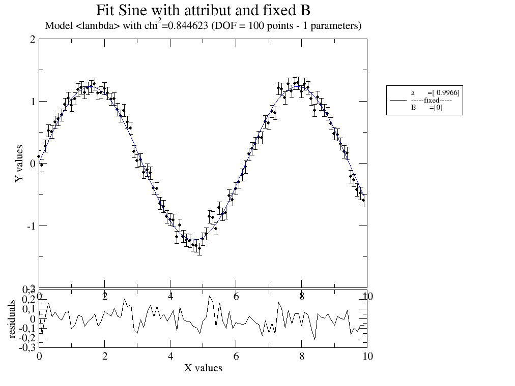
# Fit sine to simulated data using an attribute in data with different name and fixed B
data = js.dA(np.c_[x, 1.234 * np.sin(x) + 0.1 * np.random.randn(len(x)), x * 0 + 0.1].T) # create data
data.dd = 1.234 # add attribute
data.fit(sinus, {'a': 1.2, }, {'B': 0}, {'x': 'X', 'A': 'dd'}) # fit data
data.showlastErrPlot() # show fit
data.errPlotTitle('Fit Sine with attribute and fixed B')
12.3.2. 2D fit with attributes
A 2D fit using the attribute B stored in the dataArray of a dataList as second dimension.
We use dataList for fitting. This might be extended to several attributes allowing multidimensional fitting. See also Simple diffusion fit of not so simple diffusion case
# Fit sine to simulated dataList using an attribute in data with different name
# and fixed B from data.
# first one common parameter then as parameter list
# create data
data = js.dL()
ef = 0.1 # increase this to increase error bars of final result
for ff in [0.001, 0.4, 0.8, 1.2, 1.6]:
data.append(js.dA(np.c_[x, (1.234 + ff) * np.sin(x + ff) + ef * ff * np.random.randn(len(x)), x * 0 + ef * ff].T))
data[-1].B = 0.2 * ff / 2 # add attributes
# fit with a single parameter for all data, obviously wrong result
data.fit(lambda x, A, a, B, p: A * np.sin(a * x + p) + B, {'a': 1.2, 'p': 0, 'A': 1.2}, {}, {'x': 'X'})
data.showlastErrPlot() # show fit
data.errPlotTitle('Fit Sine with attribute and common fit parameter')
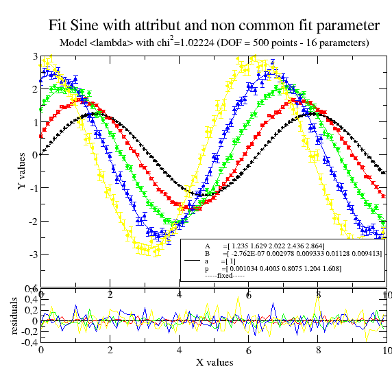
# now allowing multiple p,A,B as indicated by the list starting value
data.fit(lambda x, A, a, B, p: A * np.sin(a * x + p) + B, {'a': 1.2, 'p': [0], 'B': [0, 0.1], 'A': [1]}, {}, {'x': 'X'})
data.errPlotTitle('Fit Sine with attribute and non common fit parameter')
# plot p against A , just as demonstration
p = js.grace()
p.plot(data.A, data.p, data.p_err, sy=[1, 0.3, 1])
p.xaxis(label='Amplitude')
p.yaxis(label='phase')
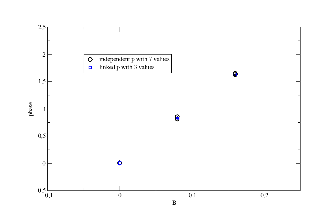
12.3.3. 2D fit with attributes and linked parameter
A 2D fit as above but the fit parameter is linked to the attribute B that
apears several times with the same value.
In experimental data this might be a repeated measurement with a different intensity
for the same process.
We get only as many fit parameters as we have unique values for B (here 3 different values).
Important is to link by adding ‘B’ in {..., 'p':[0, 'B'], ...} to the list of starting values.
#
import jscatter as js
import numpy as np

# create data. B will appear several times with same value
data = js.dL()
x = np.r_[0:10:0.1]
ef = 0.1  # increase this to increase error bars of final result
for ff in [0.001, 0.8, 1.6]:
    data.append(js.dA(np.c_[x, (1.234 + ff) * np.sin(x + ff) + ef * ff * np.random.randn(len(x)), x * 0 + ef * ff].T))
    data[-1].B = 0.2 * ff / 2  # add attributes
    # add same but different amplitude A, same phase p
    data.append(js.dA(np.c_[x, (0.234 + ff) * np.sin(x + ff) + ef * ff * np.random.randn(len(x)), x * 0 + ef * ff].T))
    data[-1].B = 0.2 * ff / 2  # add attributes

data.append(js.dA(np.c_[x, (0.234 + ff) * np.sin(x + ff) + ef * ff * np.random.randn(len(x)), x * 0 + ef * ff].T))
data[-1].B = 0.2 * ff / 2  # add attributes


# create model
model = lambda x, A, a, B, p: A * np.sin(a * x + p) + B

# plot for result
p = js.grace()

# fit with independent parameters for all dataList elements
data.fit(model, {'a': 1.2, 'p': [0], 'A': [1.2]}, {}, {'x': 'X'})

# plot p against unique B
p.plot(data.B, data.p, data.p_err, sy=[1, 1, 1], legend='independent p with 7 values')

# now A still independent but we link 'p' to 'B'
data.fit(model, {'a': 1.2, 'p': [0, 'B'], 'A': [1]}, {}, {'x': 'X'})

# plot p against unique B with less values in p
p.plot(data.B.unique, data.p, data.p_err, sy=[2, 0.7, 4], le='linked p with 3 values')
p.xaxis(label='B', min=-0.1, max=0.25)
p.yaxis(label='phase',min=-0.5,max=2.5)
p.legend(x=-0.05,y=2)
p.save('SinusoidalFit_linkedParameter.png')
12.3.4. 2D fitting using .X, .Z, .W
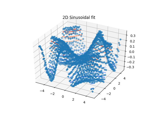
Unlike the previous we use here data with two dimensions in .X,.Z coordinates (optional .W for 3D). We use dataArray for fitting. Additional one could use again attributes to increase dimesion. This mainly depends on the data.
Another example is shown in Fitting the 2D scattering of a lattice.
import jscatter as js
import numpy as np

# 2D fit data with an X,Z grid data and Y values (For 3D we would use X,Z,W )
# For 2D fit we calc Y values from X,Z coordinates (only for scalar Y data).
# For fitting we need data with X,Z,Y columns indicated .

#  We create synthetic 2D data with X,Z axes and Y values as Y=f(X,Z)
# This is ONE way to make a grid. For fitting it can be unordered, non-gridded X,Z data
x, z = np.mgrid[-5:5:0.25, -5:5:0.25]
xyz = js.dA(np.c_[x.flatten(), z.flatten(), 0.3 * np.sin(x * z / np.pi).flatten() + 0.01 * np.random.randn(
    len(x.flatten())), 0.01 * np.ones_like(x).flatten()].T)
# set columns where to find X,Z coordinates and Y values and eY errors )
xyz.setColumnIndex(ix=0, iz=1, iy=2, iey=3)


# define model
def ff(x, z, a, b):
    return a * np.sin(b * x * z)


xyz.fit(model=ff, freepar={'a': 1, 'b': 1 / 3.}, fixpar={}, mapNames={'x': 'X', 'z': 'Z'})

# show in 2D plot
import matplotlib.pyplot as plt
from matplotlib import cm

fig = plt.figure()
ax = fig.add_subplot(111, projection='3d')
ax.set_title('2D Sinusoidal fit')
# plot data as points
ax.scatter(xyz.X, xyz.Z, xyz.Y)
# plot fit as contour lines
ax.tricontour(xyz.lastfit.X, xyz.lastfit.Z, xyz.lastfit.Y, cmap=cm.coolwarm, antialiased=False)
plt.show(block=False)
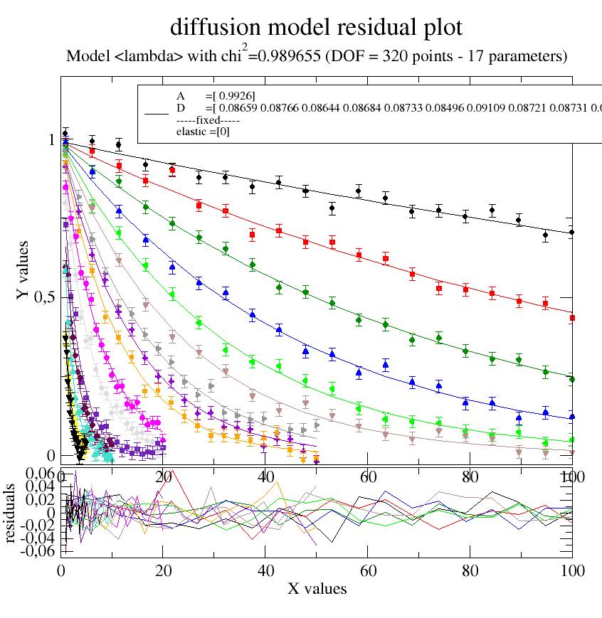
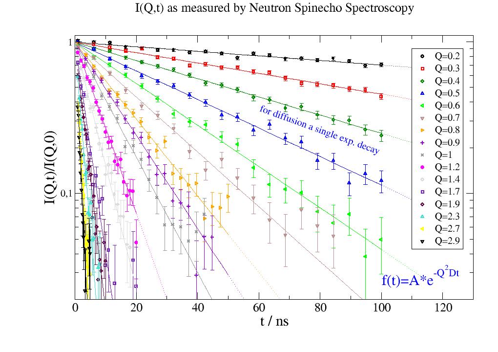
12.3.5. Simple diffusion fit of not so simple diffusion case
Here the long part with description from the first example.
This is the diffusion of a protein in solution. This is NOT constant as for Einstein diffusion.
These simulated data are similar to data measured by Neutron Spinecho Spectroscopy, which measures on the length scale
of the protein and therefore also rotational diffusion contributes to the signal.
At low wavevectors additional the influence of the structure factor leads to an upturn,
which is neglected in the simulated data.
To include the correction \(D_T(q)=D_{T0} H(q)/S(q)\) look at hydrodynamicFunct().
For details see this tutorial review Biehl et al. Softmatter 7,1299 (2011)
A key point for a simultaneous combined fit is that each dataArray has an individual ‘q’ which is used in the fit model as ‘wavevector’.
# import jscatter and numpy
import numpy as np
import jscatter as js

# read the data (16 dataArrays) with attributes as q, Dtrans .... into dataList
i5 = js.dL(js.examples.datapath + '/iqt_1hho.dat')

# define a model for the fit
diffusion = lambda A, D, t, wavevector, e=0: A*np.exp(-wavevector**2*D*t) + e

# do the fit
# single valued start parameters are the same for all 16 dataArrays
# list start parameters [...] indicate independent fitting for dataArrays
# the command line shows progress and the final result, which is found in i5.lastfit
i5.fit(model=diffusion,                         # the fit function
       freepar={'D': [0.08], 'A': 0.98},        # free start parameters
       fixpar={'e': 0.0},                       # fixed parameters
       mapNames={'t': 'X', 'wavevector': 'q'})  # map names from model to data

# open plot with results and residuals
i5.showlastErrPlot(yscale='l')

# open a plot with fixed size and plot data and fit result
p = js.grace(1.2, 0.8)
# plot the data with Q values in legend as symbols
p.plot(i5, symbol=[-1, 0.4, -1], legend='Q=$q')
# plot fit results in lastfit as lines without symbol or legend
p.plot(i5.lastfit, symbol=0, line=[1, 1, -1])
# extend to longer times by changing a model parameter (points)
p.plot(i5.modelValues(t=np.r_[10:120:5]), symbol=0, line=[2, 1, -1])

# pretty up if needed
p.yaxis(min=0.02, max=1.1, scale='log', charsize=1.5, label='I(Q,t)/I(Q,0)')
p.xaxis(min=0, max=130, charsize=1.5, label='t / ns')
p.legend(x=110, y=0.9, charsize=1)
p.title('I(Q,t) as measured by Neutron Spinecho Spectroscopy', size=1.3)
p.text('for diffusion a single exp. decay', x=60, y=0.35, rot=360 - 20, color=4)
p.text(r'f(t)=A*e\S-Q\S2\N\SDt', x=100, y=0.025, rot=0, charsize=1.5)

if 1:  # optional; save in different formats
    p.save('DiffusionFit.agr')
    p.save('DiffusionFit.png')
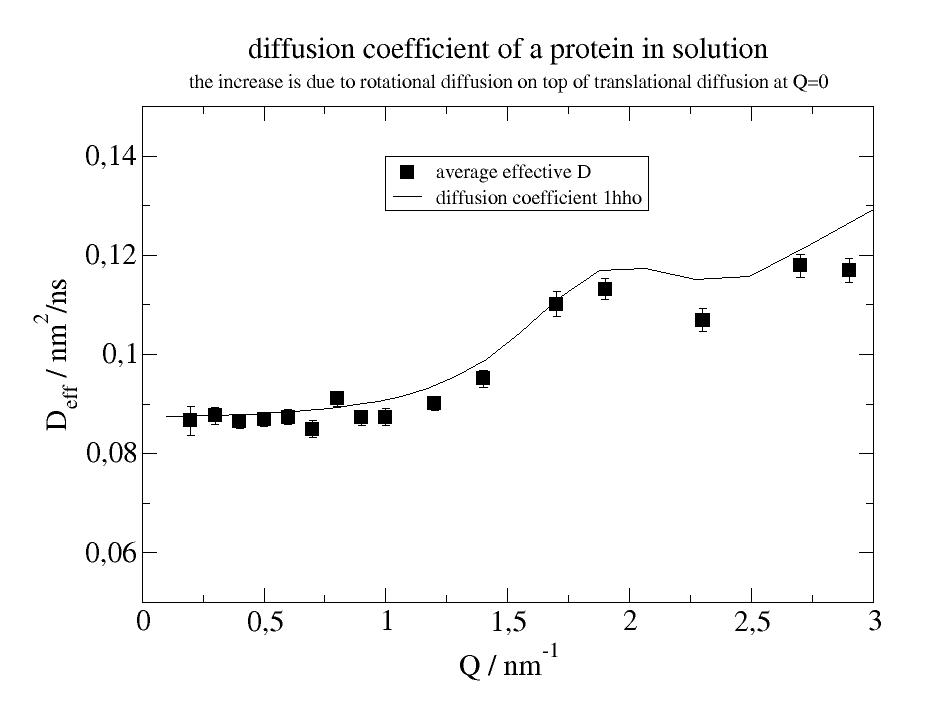
# This is the basis of the simulated data above
D = js.dA(js.examples.datapath + '/1hho.Dq')

# Plot the result in an additional plot
p1 = js.grace(1, 1)  # plot with a defined size
p1.plot(i5.q, i5.D, i5.D_err, symbol=[2, 1, 1, ''], legend='average effective D')
p1.plot(D.X, D.Y * 1000., sy=0, li=1, legend='diffusion coefficient 1hho')
# pretty up if needed
p1.title('diffusion constant of a dilute protein in solution', size=1.5)
p1.subtitle('the increase is due to rotational diffusion on top of translational diffusion at Q=0', size=1)
p1.xaxis(min=0, max=3, charsize=1.5, label=r'Q / nm\S-1')  # xaxis numbers in size 1.5
p1.yaxis(min=0.05, max=0.15, charsize=1.5, label=r'D\seff\N / nm\S2\N/ns')
p1.legend(x=1, y=0.14)

if 1:
    p1.save('effectiveDiffusion.agr')
    p1.save('effectiveDiffusion.png')
12.3.6. A long example for diffusion and how to analyze step by step
This is a long example to show possibilities.
A main feature of the fit is that we can change from a constant fit parameters to a parameter dependent one by simply changing A to [A].
import jscatter as js
import numpy as np

# load example data and show them in a nice plot as
i5 = js.dL(js.examples.datapath + '/iqt_1hho.dat')

# make a fixed size plot with the data
p = js.grace(1.5, 1)
p.plot(i5, symbol=[-1, 0.4, -1], legend='Q=$q')
p.legend(charsize=1.)
p.yaxis(0.01, 1.1, scale='log', charsize=1.5, label='I(Q,t)/I(Q,0)')
p.title('Intermediate scattering function', size=2)
p.xaxis(charsize=1.5, label='t / ns')

# defining model to use in fit
# simple diffusion
diffusion = lambda A, D, t, wavevector, elastic=0: A * np.exp(-wavevector ** 2 * D * t) + elastic
# or if you want to include in a library with description
# see examples in formel and formfactor

# in the data we have X as coordinate for time so we have to map the name
# same for the wavevector which is usually 'q' in these data
# the wavevector is available in the data for all i as i5[i].q
# or as a list as i5.q
# so test these

# analyzing the data
# to see the results we open an errorplot with Y-log scale
i5.makeErrPlot(yscale='l')
# '----------------------------------------'
# ' a first try model which is bad because of fixed high elastic fraction'
i5.fit(model=diffusion,
       freepar={'D': 0.1, 'A': 1},
       fixpar={'elastic': 0.5},
       mapNames={'t': 'X', 'wavevector': 'q'})
# '--------------------------------------'
# ' Now we try it with constant D and a worse A as starting parameters'
i5.fit(model=diffusion,
       freepar={'D': 0.1, 'A': 18},
       fixpar={'elastic': 0.0},
       mapNames={'t': 'X', 'wavevector': 'q'})
print(i5.lastfit.D, i5.lastfit.D_err)
print(i5.lastfit.A, i5.lastfit.A_err)
# A is close to 1 (as it should be here) but the fits don't look good
# '--------------------------------------'
# ' A free amplitude dependent on wavevector might improve '
i5.fit(model=diffusion,
       freepar={'D': 0.1, 'A': [1]},
       fixpar={'elastic': 0.0},
       mapNames={'t': 'X', 'wavevector': 'q'})
# and a second plot to see the results of A
pr = js.grace()
pr.plot(i5.lastfit.wavevector, i5.lastfit.A, i5.lastfit.A_err, legend='A')
# The fit is ok only the chi^2 is to high in this case of simulated data
# '--------------------------------------'
# ' now with free diffusion coefficient dependent on wavevector; is this the best solution?'
i5.fit(model=diffusion,
       freepar={'D': [0.1], 'A': [1]},
       fixpar={'elastic': 0.0},
       mapNames={'t': 'X', 'wavevector': 'q'})

pr.clear()  # removes the old stuff
pr.plot(i5.lastfit.wavevector, i5.lastfit.D, i5.lastfit.D_err, legend='D')
pr.plot(i5.lastfit.wavevector, i5.lastfit.A, i5.lastfit.A_err, legend='A')
# Ahh
# Now the amplitude is nearly constant and the diffusion is changing
# the fit is ok
# '--------------------------------------'
# ' now with changing diffusion and constant amplitude '
i5.fit(model=diffusion,
       freepar={'D': [0.1], 'A': 1},
       fixpar={'elastic': 0.0},
       mapNames={'t': 'X', 'wavevector': 'q'})
pr.clear()  # removes the old stuff
pr.plot(i5.lastfit.wavevector, i5.lastfit.D, i5.lastfit.D_err, legend='D')

# Booth fits are very good, but the last has less parameter.
# From simulation i know it should be equal to 1 for all amplitudes :-))))).
12.3.7. Fitting a multiShellcylinder in various ways
import jscatter as js
import numpy as np

# Can we trust a fit?

# simulate some data with noise
# in reality read some data
x = js.loglist(0.1, 7, 1000)
R1 = 2
R2 = 2
L = 20
# this is a three shell cylinder with the outer as a kind of "hydration layer"
simcyl = js.ff.multiShellCylinder(x, L, [R1, R2, 0.5], [4e-4, 2e-4, 6.5e-4], solventSLD=6e-4)

p = js.grace()
p.plot(simcyl, li=1, sy=0)
# noinspection PyArgumentList
simcyl.Y += np.random.randn(len(simcyl.Y)) * simcyl.Y[simcyl.X > 4].mean()
simcyl = simcyl.addColumn(1, simcyl.Y[simcyl.X > 4].mean())
simcyl.setColumnIndex(iey=2)
p.plot(simcyl, li=0, sy=1)
p.yaxis(min=2e-7, max=0.1, scale='l')


# create a model to fit
# We use the model of a double cylinder with background (The intention is to use a wrong but close model).

def dcylinder(q, L, R1, R2, b1, b2, bgr):
    # assume D2O for the solvent
    result = js.ff.multiShellCylinder(q, L, [R1, R2], [b1 * 1e-4, b2 * 1e-4], solventSLD=6.335e-4)
    result.Y += bgr
    return result


simcyl.makeErrPlot(yscale='l')
simcyl.fit(dcylinder,
           freepar={'L': 20, 'R1': 1, 'R2': 2, 'b1': 2, 'b2': 3},
           fixpar={'bgr': 0},
           mapNames={'q': 'X'})


# There are still systematic deviations in the residuals due to the missing layer
# but the result is very promising
# So can we trust such a fit :-)
# The outer 0.5 nm layer modifies the layer thicknesses and scattering length density.
# Here prior knowledge about the system might help.

def dcylinder3(q, L, R1, R2, R3, b1, b2, b3, bgr):
    # assume D2O for the solvent
    result = js.ff.multiShellCylinder(q, L, [R1, R2, R3], [b1 * 1e-4, b2 * 1e-4, b3 * 1e-4], solventSLD=6.335e-4)
    result.Y += bgr
    return result


simcyl.makeErrPlot(yscale='l')
try:
    # The fit will need quite long and fails as it runs in a wrong direction.
    simcyl.fit(dcylinder3,
               freepar={'L': 20, 'R1': 1, 'R2': 2, 'R3': 2, 'b1': 2, 'b2': 3, 'b3': 0},
               fixpar={'bgr': 0},
               mapNames={'q': 'X'}, max_nfev=3000)
except:
    # this try : except is only to make the script run as it is
    pass

# Try the fit with a better guess for the starting parameters.
# Prior knowledge by a good idea what is fitted helps to get a good result and
# prevents from running in a wrong minimum of the fit.

simcyl.fit(dcylinder3,
           freepar={'L': 20, 'R1': 2, 'R2': 2, 'R3': 0.5, 'b1': 4, 'b2': 2, 'b3': 6.5},
           fixpar={'bgr': 0}, ftol=1e-5,
           mapNames={'q': 'X'}, condition=lambda a: a.X < 4)

# Finally look at the errors.
# Was the first the better model with less parameters as we cannot get all back due to the noise in the "measurement"?
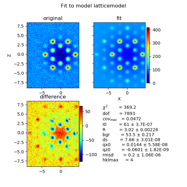
12.3.8. Fitting the 2D scattering of a lattice
This example shows how to fit a 2D scattering pattern as e.g. measured by small angle scattering.
As a first step one should fit radial averaged data to limit the lattice constants to reasonable ranges and deduce reasonable values for background and other parameters.
Because of the topology of the problem with a large plateau and small minima most fit algorithm (using a gradient) will fail. One has to take care that the first estimate of the starting parameters (see above) is already close to a very good guess or one may use a method to find a global minimum as differential_evolution or brute force scanning. This requires some time.
In the following we limit the model to a few parameters. One needs basically to include more as e.g. the orientation of the crystal in 3D and more parameters influencing the measurement. Prior knowledge about the experiment as e.g. a preferred orientation during a shear experiment is helpful information.
Another possibility is to normalize the data e.g. to peak maximum=1 with high q data also fixed.
As a good practice it is useful to first fit 1D data to fix some parameters and add e.g. orientation in a second step with 2D fitting.
import jscatter as js
import numpy as np
# load a image with hexagonal peaks (synthetic data)
image = js.sas.sasImage(js.examples.datapath + '/2Dhex.tiff')
image.setPlaneCenter([51, 51])
image.gaussianFilter()
# transform to dataarray with X,Z as wavevectors
# The fit algorithm works also with masked areas
hexa = image.asdataArray(0)
def latticemodel(qx, qz, R, ds, rmsd, hklmax, bgr, I0, qx0=0, qz0=0):
# a hexagonal grid with background, domain size and Debye Waller-factor (rmsd)
# 3D wavevector
qxyz = np.c_[qx + qx0, qz - qz0, np.zeros_like(qx)]
# define lattice
grid = js.sf.hcpLattice(R, [3, 3, 3])
# here one may rotate the crystal
# calc scattering
lattice = js.sf.orientedLatticeStructureFactor(qxyz, grid, domainsize=ds, rmsd=rmsd, hklmax=hklmax)
# add I0 and background
lattice.Y = I0 * lattice.Y + bgr
return lattice
# Because of the high plateau in the chi2 landscape
# we first need to use a algorithm finding a global minimum
# this needs some time and maybe a good choice of starting parameters
if 0:
# Please do this if you want to wait
hexa.fit(latticemodel, {'R': 3, 'ds': 10, 'rmsd': 0.3, 'bgr': 16, 'I0': 90},
{'hklmax': 5, }, {'qx': 'X', 'qz': 'Z'}, method='differential_evolution')
#
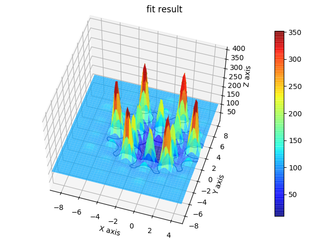
fig = js.mpl.surface(hexa.X, hexa.Z, hexa.Y, image.shape)
fig = js.mpl.surface(hexa.lastfit.X, hexa.lastfit.Z, hexa.lastfit.Y, image.shape)
# We use as starting parameters the result of the previous fit
# Now we use LevenbergMarquardt algorithm to polish the result
hexa.fit(latticemodel, {'R': 3.02, 'ds': 8.3, 'rmsd': 0.27, 'bgr': 19, 'I0': 95, 'qx0': 0, 'qz0': 0},
{'hklmax': 4, }, {'qx': 'X', 'qz': 'Z'}, diff_step=0.01)
fig = js.mpl.showlastErrPlot2D(hexa, shape=image.shape, transpose=1)
fig2 = js.mpl.surface(hexa.lastfit.X, hexa.lastfit.Z, hexa.lastfit.Y, image.shape)
fig2.suptitle('fit result')
12.3.9. Using cloudscattering as fit model
At the end a complex shaped object: A cube decorated with spheres of different scattering length.
# Using cloudScattering as fit model.
# We have to define a model that parametrize the building of the cloud that we get a fit parameter.
# As example we use two overlapping spheres. The model can be used to fit some data.
import jscatter as js
import numpy as np
#: test if distance from point on X axis
isInside = lambda x, A, R: ((x - np.r_[A, 0, 0]) ** 2).sum(axis=1) ** 0.5 < R
#: model
def dumbbell(q, A, R1, R2, b1, b2, bgr=0, dx=0.3, relError=100):
# A sphere distance
# R1, R2 radii
# b1,b2 scattering length
# bgr background
# dx grid distance not a fit parameter!!
mR = max(R1, R2)
# xyz coordinates
grid = np.mgrid[-A / 2 - mR:A / 2 + mR:dx, -mR:mR:dx, -mR:mR:dx].reshape(3, -1).T
insidegrid = grid[isInside(grid, -A / 2., R1) | isInside(grid, A / 2., R2)]
# add blength column
insidegrid = np.c_[insidegrid, insidegrid[:, 0] * 0]
# set the corresponding blength; the order is important as here b2 overwrites b1
insidegrid[isInside(insidegrid[:, :3], -A / 2., R1), 3] = b1
insidegrid[isInside(insidegrid[:, :3], A / 2., R2), 3] = b2
# and maybe a mix ; this depends on your model
insidegrid[isInside(insidegrid[:, :3], -A / 2., R1) & isInside(insidegrid[:, :3], A / 2., R2), 3] = (b2 + b1) / 2.
# calc the scattering
result = js.ff.cloudScattering(q, insidegrid, relError=relError)
result.Y += bgr
# add attributes for later usage
result.A = A
result.R1 = R1
result.R2 = R2
result.dx = dx
result.bgr = bgr
result.b1 = b1
result.b2 = b2
result.insidegrid = insidegrid
return result
#
# test it
q = np.r_[0.01:10:0.02]
data = dumbbell(q, 4, 2, 2, 0.5, 1.5)
#
# Fit your data like this (I know that b1 abd b2 are wrong).
# It may be a good idea to use not the highest resolution in the beginning because of speed.
# If you have a good set of starting parameters you can decrease dx.
data2 = data.prune(number=200)
data2.makeErrPlot(yscale='l')
data2.setlimit(A=[0, None, 0])
data2.fit(model=dumbbell,
freepar={'A': 3},
fixpar={'R1': 2, 'R2': 2, 'dx': 0.3, 'b1': 0.5, 'b2': 1.5, 'bgr': 0},
mapNames={'q': 'X'})
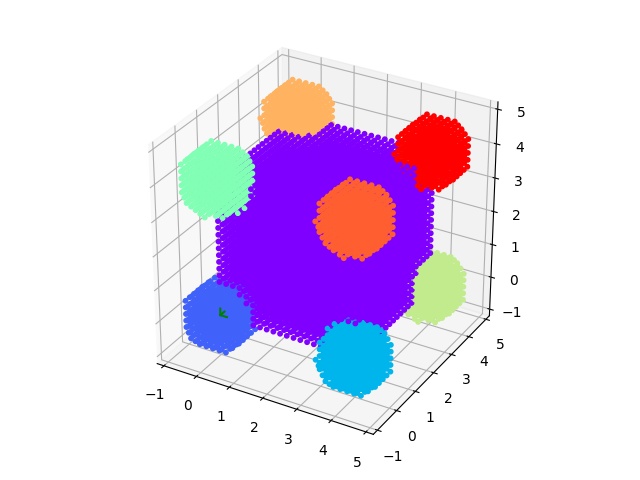
# An example to demonstrate how to build a complex shaped object with a simple cubic lattice
# Methods are defined in lattice objects.
# A cube with the corners decorated by spheres
import jscatter as js
import numpy as np
grid = js.sf.scLattice(0.2, 2 * 15, b=[0])
v1 = np.r_[4, 0, 0]
v2 = np.r_[0, 4, 0]
v3 = np.r_[0, 0, 4]
grid.inParallelepiped(v1, v2, v3, b=1)
grid.inSphere(1, center=[0, 0, 0], b=2)
grid.inSphere(1, center=v1, b=3)
grid.inSphere(1, center=v2, b=4)
grid.inSphere(1, center=v3, b=5)
grid.inSphere(1, center=v1 + v2, b=6)
grid.inSphere(1, center=v2 + v3, b=7)
grid.inSphere(1, center=v3 + v1, b=8)
grid.inSphere(1, center=v3 + v2 + v1, b=9)
fig = grid.show()
js.mpl.show()
12.3.10. Bayesian inference for fitting
method=’bayes’ uses Bayesian inference for modeling and the MCMC algorithms for sampling (we use emcee). Requires a larger amount of function evaluations but returns errors from Bayesian statistical analysis and allows inclusion of prior knowledge about parameters and restrictions.
For Bayesian analysis the log probability \(\ln\,p(y\,|\,x,\sigma,a) + ln(p(a_j))\) is maximized with the log likelihood \(ln (p(y\,|\,x,\sigma,a))\) and the prior \(p(a_j)\). Asuming Gaussian statistics we use
By default an uniform (so-called “uninformative”) prior is used
which can be changed using the parameter ln_prior to be more informative.
Assuming for parameter \(a_j\) a Gaussian distribution of deviations from a mean with width sigma
where for \(\lambda=0\) the prior vanishes.
\(\lambda\) quantifies of by how much we believe that e.g. \(w_j = a_j-a_{mean}\) should be close to zero and can be choosen as \(\lambda=n 0.5/\sigma^2\) assuming that \(a_j\) shoud be within a Gaussian of width sigma, maybe determined from a different measurement.
The scale \(n\) scales the Gaussian that the weight is comparable to the log likelihood. Using \(\lambda=0.5/\sigma^2\) weights the constrain equal to one datapoint.
In general the \(p(a_j)\) depend only on fit parameters \(a_j\) and not on \(Y_i\) or \(f(X_i,...)\). To allow more complex constraints, e.g. fitting a protein structure with the constrain that the backbone is not overstretched, the modelValues can be accessed if log_prior uses the keyword ‘modelValues’. Also the weigthed squared errors \(\chi^2_i=\frac{[Y_i-f(X_i,a_1,..a_p)]^2}{\sigma_i^2}\) can be accessed using the keyword ‘x2i’ to regularise in some way different meassurements according to their errors.
The example shows how some knowledge about parameters A and D that can be used for the prior. We assume here that the amplitude A is distributed around 1 within a Gaussian distribution and D around 0.09.
The evaluation might take somewhat longer for bayes (here 100s on my desktop).
import numpy as np
import jscatter as js
import matplotlib.pyplot as plt
import corner

# data to fit
# We use each a subset to speed up the example
i5 = js.dL(js.examples.datapath+'/iqt_1hho.dat')[[3, 5]]

# model
def diffusion(A, D, t, elastic, wavevector=0):
    return A*np.exp(-wavevector**2*D*t) + elastic

# Define ln_prior that describes knowledge about the data, parameters or how parameters are distributed.
# The ln_prior is complemented by the limits as:
# 0 within limits (log(1)) and -inf outside limits (log(0))
# Without prior only the limits are used (uninformative prior) that
# the prior is optional if you know something about the parameters.

# As the prior is a probability it should be normalized. On the other side, as in the examples,
# the normalisation constants result in constant offset dependent on sigma
# and will not influence the best fit result but chi2.

# To be compatible with regularisation the ln_prior is written here as positive and
# internally  multiplied by `-1`.

Amean, Asig = 1.0 , 0.01
Dmean, Dsig = 0.09 , 0.02
def ln_priorGAUSS(A, D):
    # assuming a normalized Gaussian distribution around the mean of A and D with width sig (Gaussian prior)
    # https://en.wikipedia.org/wiki/Normal_distribution
    # the log of the Gaussian is the log_prior, the second log is from the Gaussian normalisation
    # negative sign like common literature
    # the parameters are arrays for all elements of the dataList or a float for common parameters
    # the 't' is not included as it describes the .X values, 'elastic' is not used (no knowledge about it).
    lp = -0.5 * np.sum((A-Amean)**2/Asig**2) - (0.5 * np.log(2*np.pi) + np.log(Asig)) * len(A)
    lp += -0.5 * np.sum((D-Dmean)**2/Dsig**2) - (0.5 * np.log(2*np.pi) + np.log(Dsig)) * len(D)
    # return negative to be regularisation compatible
    return -lp

# as example => Laplace prior.
# The Laplace prior has fatter tails than the Gaussian, and is also more concentrated around zero.
def ln_priorLAPLACE(A, D):
    # while Gauss uses L2 norm , here we use L1 norm =>|A-Amean|
    # https://en.wikipedia.org/wiki/Laplace_distribution
    lp = -  np.sum(np.abs(A-Amean)/(2**0.5*Asig)) + np.log(1/(2*2**0.5*Asig)*len(A))
    lp += - np.sum(np.abs(D-Dmean)/2**0.5*Dsig) + np.log(1/(2*2**0.5*Dsig)*len(D))
    # return negative to be regularisation compatible
    return -lp

i5.setlimit(D=[0.05, 1], A=[0.5, 1.5])

# do Bayesian analysis with the prior
i5.fit(model=diffusion, freepar={'D': [0.2], 'A': 0.98}, fixpar={'elastic': 0.0},
      mapNames={'t': 'X', 'wavevector': 'q'}, condition=lambda a: a.X<90,
       method='bayes', tolerance=20, bayesnsteps=1000, ln_prior=ln_priorGAUSS)

i5.showlastErrPlot()

# get sampler chain and examine results removing burn in time 2*tau
tau = i5.getBayesSampler().get_autocorr_time(tol=20)
flat_samples = i5.getBayesSampler().get_chain(discard=int(2*tau.max()), thin=1, flat=True)
labels = i5.getBayesSampler().parlabels

plt.ion()
fig = corner.corner(flat_samples, labels=labels, quantiles=[0.16, 0.5, 0.84], show_titles=True, title_fmt='.3f')
plt.show()
# fig.savefig(js.examples.imagepath+'/bayescorner_withprior.jpg')
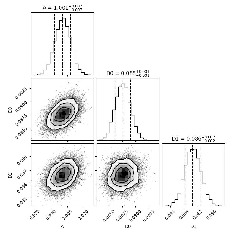
If we neglect the normalisation terms -ln_prior is the regularisation term used below.
12.3.11. Regularisation for fitting
Regularisation in least squares offers the posibility to use prior knowledge similar to ‘bayes’ to constrain the solution. Different to ‘bayes’ it uses the faster \(\chi^2 minimization\) algorithms with the additional constrain \(\propto ln(p(w))\). For a Gaussian prior \(p(w)\) corresponds to ridge regression and for a Laplace prior to Lasso regression . You can define whatever you want (some things are more justified than others) as long as there is a minimum and \(ln(p(w))>0\).
For \(\chi^2 minimization\) we minimise \(\chi_{red}^2 - ln(p(a_j))\). For a Gaussian prior (Ridge regression) this is
where for \(\lambda=0\) the conventional \(\chi_{red}^2 minimization\) is retrieved.
\(\lambda\) quantifies of by how much we believe that e.g. \(w_i = A-A_{mean}\) should be close to zero and can be choosen as \(\lambda=\frac{1}{n}0.5/\sigma^2\) similar to the above ln_prior assuming that A shoud be within a Gaussian of width sigma, maybe determined from a different measurement.
Selects the weight you want to apply :
Using \(\lambda=0.5/\sigma^2\) for a single variable in Gaussian distribution would be weighted like all measurement values in \(\chi_{red}^2\) together.
A divisor 1/n scales the Gaussian that the weight is comparable to one data point.
Weighing with \(1/n_{j}\) weight each \(w_j\) like \(\chi_{red}^2\).
If the \(\lambda \sum_j w_j^2\) are to strong weigthed, this will dominate the result.
For the below example with i5 containing 16 Q values with about 20 points a weight equal to 20 points corresponding to one Q might be reasonable.
In general the \(p(a_j)\) depend only on fit parameters \(a_j\) and not on \(Y_i\) or \(f(X_i,...)\). The best \(\lambda\) may be selected from a series of tries as the one with best fit results.
To allow more complex constraints the modelValues can be accessed if log_prior uses the keyword modelValues.
The weigthed squared errors \(\chi^2_i=\frac{[Y_i-f(X_i,a_1,..a_p)]^2}{\sigma_i^2}\)
can be accessed as modelValues.chi2i and degrees of freedom as modelValues.dof.
Anything calculated in the model can be accessed in modelValues.
This can be used to constrain by something calculated in the model or to weight e.g. different meassurements according to their errors, number of datapoints or relative contribution to \(\chi^2\).
The example shows how some knowledge about parameters A and D can be used for the regularisation. We assume here that the amplitude A is distributed around 1 within a Gaussian distribution and D around 0.09.
!!! The example is an example for to strong constraints. Its more how to do it and here without advantage.
import numpy as np
import jscatter as js

# data to fit
# We can fit all as it is faster than bayes
i5 = js.dL(js.examples.datapath+'/iqt_1hho.dat')

# model
def diffusion(A, D, t, elastic, wavevector=0):
    return A*np.exp(-wavevector**2*D*t) + elastic

# Define regularization function that describes knowledge about the data, parameters or how parameters are distributed.
Amean, Asig = 1.0 , 0.01
Dmean, Dsig = 0.09 , 0.02
def ln_priorGAUSS(A, D):
    # assuming a normalized Gaussian distribution around the mean of A and D with width sig (Gaussian prior)
    # the log of the Gaussian is ~ lambda*w**2 = 0.5/Asig**2 * (a-Amean)**2,
    # lambda*w**2 should be always positive without normalisation.
    # the parameters are arrays for all elements of the dataList or a float for common parameters
    # the 't' is not included as it describes the .X values, 'elastic' is not used (no knowledge about it).
    lp = 0.5 * np.sum((A-Amean)**2/Asig**2)
    lp += 0.5 * np.sum((D-Dmean)**2/Dsig**2)
    return lp

# as example => Laplace prior.
# The Laplace prior has fatter tails than the Gaussian, and is also more concentrated around zero.
def ln_priorLAPLACE(A, D):
    # while Gauss uses L2 norm , here we use L1 norm =>|A-Amean|
    lp =  np.sum(np.abs(A-Amean)/(2**0.5*Asig))
    lp += np.sum(np.abs(D-Dmean)/2**0.5*Dsig)
    return lp

# as example => Gaussian around the average only for A and usage of current modelValues.
# if ln_prior has keyword 'modelValues' these are added from the current calculation
def ln_priorMEAN(modelValues, A):
    # for a free A we want that these are within some sigma with unknown mean.
    lp =  np.sum(np.abs(A-np.mean(A))**2) / Asig**2
    # this is a stupid example as demonstration
    # e.g. in SAXS it might be I0 or Rg that determine a penalty
    # that is not in the parameters but in the formfactor calculation
    lp += 0 if modelValues.Y[:5,0].mean > 0.9 else 10

    return lp


i5.setlimit(D=[0.05, 1], A=[0.5, 1.5])

# do the fit with regression constrain in  ''ln_prior''.
i5.fit(model=diffusion, freepar={'D': [0.2], 'A': 0.98}, fixpar={'elastic': 0.0},
      mapNames={'t': 'X', 'wavevector': 'q'}, condition=lambda a: a.X<90,
      method='lm', ln_prior=ln_priorGAUSS)

i5.showlastErrPlot()

p=js.grace()
p.plot(i5.q,i5.D,i5.D_err,le='Too strong regularization')

# The result is not good as the constraint on D is too much constraining the diffusion coefficient.
# Therefore, the errors are large and the values to close to 0.09.
# better is simple 'lm' without constrain in this case.
# This was wrong knowledge assuming D is constant!

i5.fit(model=diffusion, freepar={'D': [0.2], 'A': 0.98}, fixpar={'elastic': 0.0},
       mapNames={'t': 'X', 'wavevector': 'q'}, condition=lambda a: a.X<90,
       method='lm',output=False)
p.plot(i5.q,i5.D,i5.D_err,le='LevenbergMarquardt fit')
p.legend(x=0.1,y=0.13)
p.yaxis(min=0.05,max=0.15)
12.3.12. Iterative reweighting of multiple measurements
In a combined fit of \(K\) datasets of different types, a naive summation of \(\chi^2\) contributions - assuming identical and independent distribution of deviations - causes large datasets or dataset with systematically smaller error to dominate the minimization. Reweighting corrects this by assigning each dataset a weight \(w_k\) like \(\chi^2= \sum_k w_k\chi^2_k\).
Application : As an example we might think about a NSE measurement with good defined error bars and a dynamic light scattering (DLS) measurement which typically gives no error at all for the correlation function. Here we can estimate an error for DLS and refine this estimate. Another application might be to identify dataset that need larger reweighting because of suspicious data or error estimates, e.g a large number of zero counts in bins or wrong counting during the measurement, and identify outliers.
Using different weights was introduced by [1]_ and others as Iteratively Reweighted Least-Squares (IRLS). IRLS iteratively calculates weights of individual data points and simultaneously tries to find model parameters that fit the bulk of the data using a least-squares approach, to produce estimates robust against outliers. Reweighting of datasets from different measurements was used by Larsen and Pedersen for combined fit of SAXS and SANS measyrements [2], [3].
Here we describe a iterative
Expectation-Maximization (EM) algorithm
used with the command regularizedEM()
as an iterative reweighting of different mesurements like SAXS/SANS with different contrast or combining
masurements of different instruments like neutron time of flight, backscattering and neutron spin echo
as combined in [4] or [5].
Iterative reweigthing avoids time consuming Bayesian inference by faster iteration using standard fit routines.
This is in particular useful if the model evaluation takes some time.
Excurs: Bayesian Analysis with precision hyperparameter
Bayesian Analysis
In the Bayesian framework the combined fit is formulated as a posterior distribution over the model parameters \(\theta\) and per-dataset precision hyperparameters \(\alpha_k\):
where the Gaussian likelihood for dataset \(k\) is
and \(\alpha_k\) rescales the trustworthiness of dataset \(k\) — large \(\alpha_k\) means the dataset is weighted heavily, small \(\alpha_k\) means it is down-weighted. Without rescaling the likelihood is only \(\ln \mathcal{L}_k(\theta)=-\frac{1}{2}\chi^2_k(\theta)\).
The conjugate prior for \(\alpha_k\) - our prior knowledge - is the Gamma distribution
whose kernel matches the likelihood in \(\alpha_k\) exactly, so the posterior on \(\alpha_k\) is also Gamma with updated parameters:
with posterior mean
Marginalizing \(\alpha_k\) out of the joint posterior yields a marginal posterior over \(\theta\) alone, in which the uncertainty of each dataset’s error calibration is propagated into the parameter estimates rather than ignored.
The prior parameters \(a_k\) and \(b_k\) control the degree of regularisation:
\(a_k = b_k = 0\) (Jeffreys): no prior knowledge; weights adapt freely to the data.
\(a_k = b_k = 2\) (weakly informative): prior mean \(\langle\alpha_k\rangle_0 = 1\), expressing the belief that stated errors are approximately correct while allowing adaptation.
\(a_k = b_k = N_k/2\) (strongly informative): prior mean 1 with variance \(\propto 1/N_k\), strongly constraining \(\alpha_k \approx 1\).
The EM-algorithm applied to a Bayesian model in which each dataset carries a precision hyperparameter \(\alpha_k \sim \mathrm{Gamma}(a_k, b_k)\) is an iterative procedure with an Expectation and a Maximization step. The general weight update at each iteration \(\nu\) using the posterior mean is
where \(N_k^{\mathrm{eff}} = N_k + 2a_k\) is an effective sample size inflated by the prior, and \(\chi^2_{\mathrm{reg},k} = 2b_k\) is a regularisation floor that prevents \(w_k\) from diverging when \({\chi^2_k}^{(\nu)} \to 0\). Convergence is guaranteed because each EM iteration increases the marginal posterior \(P(\theta \mid \mathrm{data})\).
The iterative reweighting algorithm is the EM-algorithm applied to this model: the E-step replaces \(\alpha_k\) by its posterior mean \(\langle\alpha_k\rangle\) given the current parameters, and the M-step maximises the resulting weighted cost over \(\theta\). This is equivalent to empirical Bayes — the hyperparameters \(\alpha_k\) are estimated from the data itself rather than fixed in advance.
The regularized EM-algorithm uses for \(\chi^2 minimization\) the total cost function \(C(\theta)\) (with parameters \(\theta = X_i,a_1,..a_p\))
where \(N_k\) is the number of datapoints in dataset \(k\). The total cost function is defined as the mean of per-dataset reduced \(\chi^2\) values, normalised so that a good combined fit gives \(C \approx 1\), directly analogous to the single-dataset criterion \(\chi^2_{\mathrm{red}} \approx 1\):
The iteration is initialised at the prior mean \(w_k^{(0)} = a_k/b_k\). For the Jeffreys prior the prior mean is undefined and \(w_k^{(0)} = 1\) is used as a neutral starting point. An initial M-step with these weights produces the first residuals \({\chi^2_k}^{(0)}\) from which the E-step computes the first data-informed weights.
At convergence, the fixed point condition
holds for every dataset individually, and the total cost satisfies \(\langle C \rangle = 1\).
The reweighting implies that \(\chi^2_{red} \to 1\) that it is not anymore a measure of fit quality but individual unweighted \(\chi^2_{\mathrm{red},k}\) still describe the fit quality for each dataset and can be used to determine a better error estimate (DLS above) or to identify suspicious data with high reweighting.
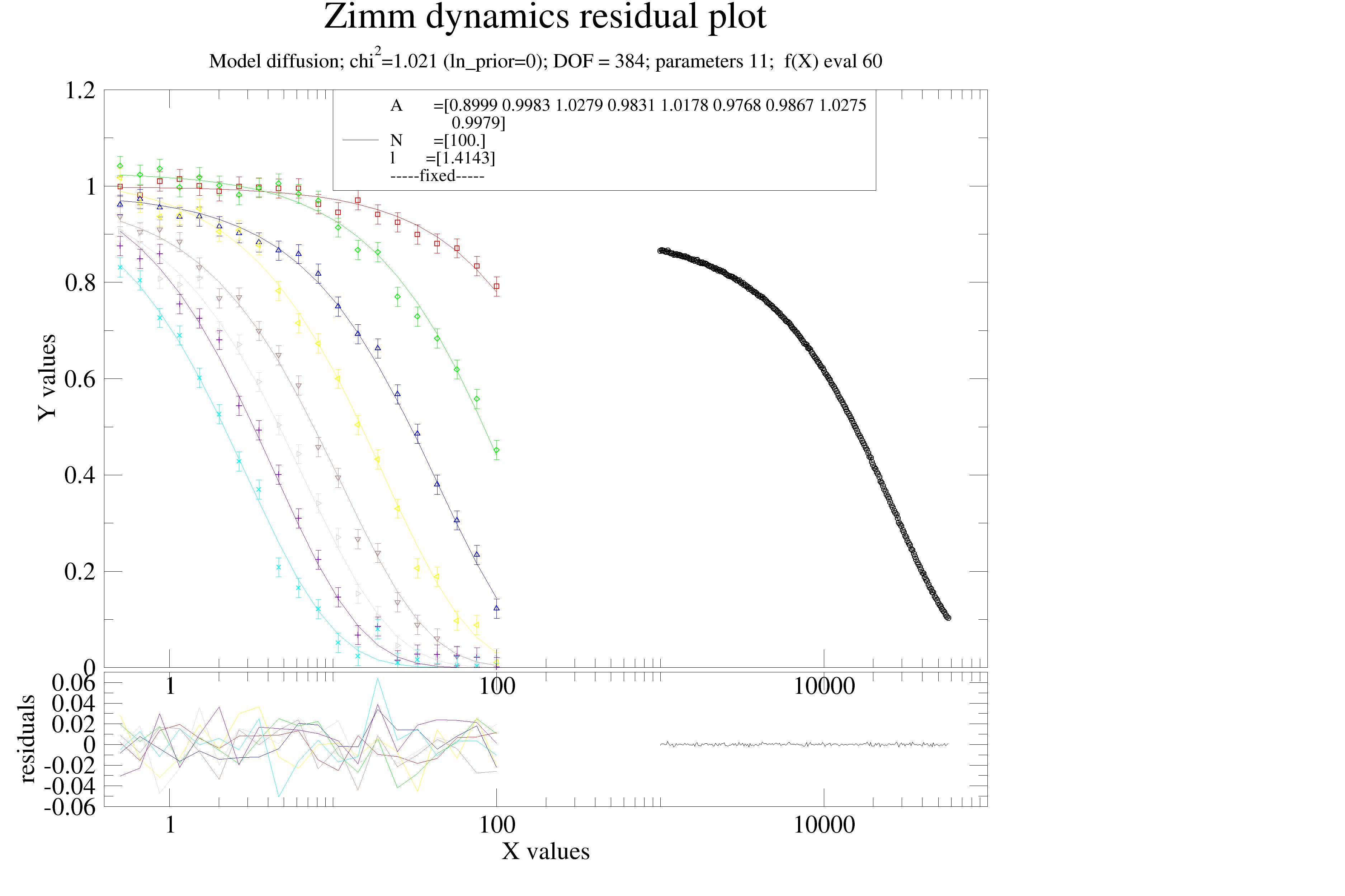
A short example: Zimm dynamics of a polymer in theta-solvent with DLS and NSE. Iterative reweighting is used to detect the wrong errors in synthetic data.
import jscatter as js
import numpy as np

def diffusion(A, t, q, N=200, l=1):
    zimm = js.dynamic.finiteZimm(t, q, N, 30, l=l, Dcm=None, tintern=0., Temp=273 + 20)
    #HP = js.dynamic.diffusionHarmonicPotential(t,q,rmsd,tau)
    zimm.Y = A * zimm.Y
    return zimm

# generate data with known properties
data = js.dL()
# typical DLS data: lambda 633 nm theta=173 degrees intercept 0.8 and cut at Y<0.1 and error 0.001
qq = 0.026
t = js.loglist(1e3,1e6,400)
diff = diffusion(0.9, t, qq)
dls = js.dA(np.c_[t, diff.Y + 0.001*np.random.randn(len(t)), t * 0 + 0.005].T)   # => errors too large
dls = dls[:,dls.Y>0.1]  # cut long times as usually done for  DLS
data.append(dls)
data[-1].q = qq
data[-1].type='dls'

# NSE data with 20 timevalues
ef = 0.02
t = js.loglist(0.5,100,20)
A = np.random.normal(1,0.02,8)
for qq,a in zip(np.r_[0.2:1.8:12j],A):
    diff = diffusion(a, t, qq)
    data.append(js.dA(np.c_[t, diff.Y + ef*np.random.randn(len(t)), t * 0 + ef].T))
    data[-1].q = qq
    data[-1].type='nse'
# ----------------------------------


# standard fit as start
data.makeErrPlot(title='Zimm dynamics residual plot', xscale='log',legpos=[0.2, 0.8])
data.fit(model=diffusion,
   freepar={'A':[1], 'N':100, 'l':2 }, fixpar={},
   mapNames={'t': 'X'},)
data.errplot[0].yaxis(min=0,max=1.2)
data.errplot[0].legend(x=10,y=1.2)
# data.savelastErrPlot(js.examples.imagepath+'/iterativeReweight.jpg',size=(2,2),dpi=200)

# check chi^2_{red,k} for each dataset
data.reducedChi2k()  # DLS chi2_k is quite small fit not bad here

# regularisation steps 3 for dataArrays
weights, convergence = data.regularizedEM(a=1,b=1, steps=3)
# weights => dls weight ~20 times smaller
# convergence bad => a=1,b=1 too strong (because of DLS)

# repeat with a=0, b=0
weights, convergence = data.regularizedEM(a=0,b=0, steps=3)
# weight ~23 as dls error is 5 times to large ~5**2=25
#
# check chi^2_{red,k} for each dataset
data.reducedChi2k()  # DLS chi2_k is quite small fit not bad here

# regularisation steps 3 for dataArrays
# here only differentiating for measurement type as ['dls',  'nse']
weights, convergence = data.regularizedEM(a=[0,'type'],b=[0], steps=3)
Regularisation with a non-informative prior
With a Jeffreys prior (non-informative prior) using \(\mathrm{Gamma}(a_k \to 0, b_k \to 0)\), the posterior mean of \(\alpha_k\) at fixed \(\theta\) is
\[\langle\alpha_k\rangle = \frac{a_k + N_k/2}{b_k + \chi^2_k/2} \xrightarrow{\,a_k,\,b_k\,\to\,0\,} \frac{N_k}{\chi^2_k} = \frac{1}{\chi^2_{\mathrm{red},k}},\]The weights are updated at each iteration \(\nu\) as \(w_k^{(\nu+1)} = 1 / {\chi^2_{\mathrm{red},k}}^{(\nu)}\). The initial weights \(w_k^{(0)} = 1\) correspond to equal weighting of all datasets in reduced \(\chi^2\) units, which is the prior expectation that all datasets are correctly normalised.
The Jeffreys case adds no information beyond what the data contain. So in the strict sense the Jeffreys EM iteration is not regularisation.
Regularisation with an informative prior
The iterative reweighting scheme can be stabilised by replacing the Jeffreys prior on \(\alpha_k\) with an informative \(\mathrm{Gamma}(a_k >0, b_k>0)\) prior. This is particularly useful for small datasets where \(\chi^2_{\mathrm{red},k}\) is noisy and the unregularised weights may fluctuate strongly between iterations.
Three natural choices of prior are summarised below. Remember that for \(\mathrm{Gamma}(a_k, b_k)\) the \(mean=a/b\) and \(\sigma^2=a/b^2\) .
Prior |
\(a_k\) |
\(b_k\) |
Effect |
|---|---|---|---|
Jeffreys (no regularisation) |
\(0\) |
\(0\) |
Weights vary freely; exact recovery of \(N_k/\chi^2_k\); can be noisy for small \(N_k\) |
Weakly informative |
\(2\) |
\(2\) |
\(\mu=1\); \(\sigma^2=1/2\); floor \(2b_k=4\); update \((N_k+4)/(\chi^2_k+4)\) |
Strongly informative |
\(N_k/2\) |
\(N_k/2\) |
\(\mu=1\); \(\sigma^2 \propto 1/N_k\); enforces \(\chi^2_{\mathrm{red},k}\approx 1\) as hard constraint |
The weakly informative choice \(a_k = b_k = 2\) is recommended as a default. It centres \(\alpha_k\) near 1, expressing the belief that the stated errors are approximately correct, while still allowing the weights to adapt if a dataset is systematically over- or under-weighted. The resulting update
differs negligibly from the Jeffreys rule for large \(N_k\), but suppresses erratic weight changes when \(N_k\) is small. The convergence criterion
still holds to within corrections of order \(2 a_k/N_k\), which vanish as \(N_k \to \infty\).
Note
For the strongly informative prior \(a_k = b_k = N_k/2\), the weight update is
and the convergence criterion evaluates to
which equals 1 only when \({\chi^2_{\mathrm{red},k}}^{(\infty)} = 1\), confirming that this prior enforces correct error calibration as a hard constraint.
Warning
If a dataset shows \(\chi^2_{\mathrm{red},k} \gg 1\) at convergence even with the strongly informative prior, this indicates model inadequacy rather than error misestimation. Per-dataset residuals should always be inspected after convergence.
12.4. References
12.5. Analysis of SAS data
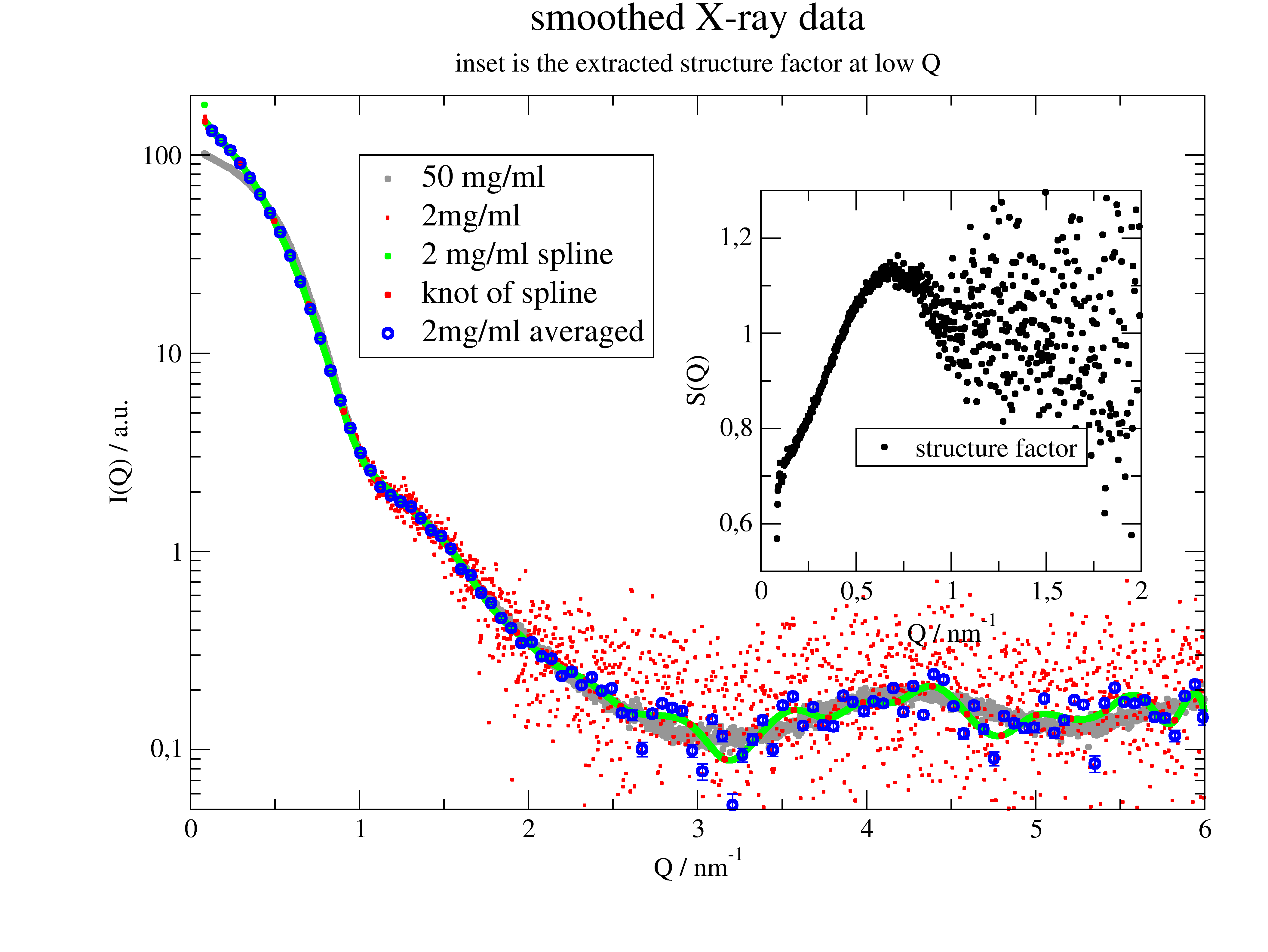
12.5.1. How to smooth Xray data and make an inset in the plot
SAS data often have a large number of points at higher Q. The best way to get reasonable statistics there is to reduce the number of points by averaging in intervals (see .prune). Spline gives trust less results.
These are real data from X33 beamline, EMBL Hamburg.
import jscatter as js
import numpy as np
from scipy.interpolate import LSQUnivariateSpline

# load data
ao50 = js.dA(js.examples.datapath + '/a0_336.dat')
ao50.conc = 50
ao10 = js.dA(js.examples.datapath + '/a0_338.dat')
ao10.conc = 2

p = js.grace(1.5, 1)
p.clear()

p.plot(ao50.X, ao50.Y, symbol=[1, 0.2, 9], legend='50 mg/ml')
p.plot(ao10.X, ao10.Y, line=0, symbol=[1, 0.05, 2], legend='2mg/ml')
p.xaxis(0, 6, label=r'Q / nm\S-1')
p.yaxis(0.05, 200, scale='logarithmic', label='I(Q) / a.u.')
p.title('smoothed X-ray data')
p.subtitle('inset is the extracted structure factor at low Q')

# smoothing with a spline
# determine the knots of the spline
# less points than data points
t = np.r_[ao10.X[1]:ao10.X[-2]:30j]
# calculate the spline
f = LSQUnivariateSpline(ao10.X, ao10.Y, t)
# calculate the new y values of the spline at the x points
ys = f(ao10.X)
p.plot(ao10.X, ys, symbol=[1, 0.2, 5, 5], legend='2 mg/ml spline ')
p.plot(t, f(t), line=0, symbol=[1, 0.2, 2, 1], legend='knot of spline')

# other idea: use lower number of points with averages in intervals
# this makes 100 intervals with average X and Y values and errors if wanted. Check prune how to use it!
# this is the best solution and additionally creates good error estimate!!!
p.plot(ao10.prune(number=100), line=0, symbol=[1, 0.5, 4], legend='2mg/ml averaged')
p.legend(x=1, y=100, charsize=1.2)
p.xaxis(0, 6)
p.yaxis(0.05, 200, scale='logarithmic')

# make a smaller plot inside for the structure factor
p.new_graph()
p[1].SetView(0.6, 0.4, 0.9, 0.8)
p[1].plot(ao50.X, ao50.Y / ao10.Y, symbol=[1, 0.2, 1, ''], legend='structure factor')
p[1].yaxis(0.5, 1.3, label='S(Q)')
p[1].xaxis(0, 2, label=r'Q / nm\S-1')
p[1].legend(x=0.5, y=0.8)

p.save('smooth_xraydata.png')
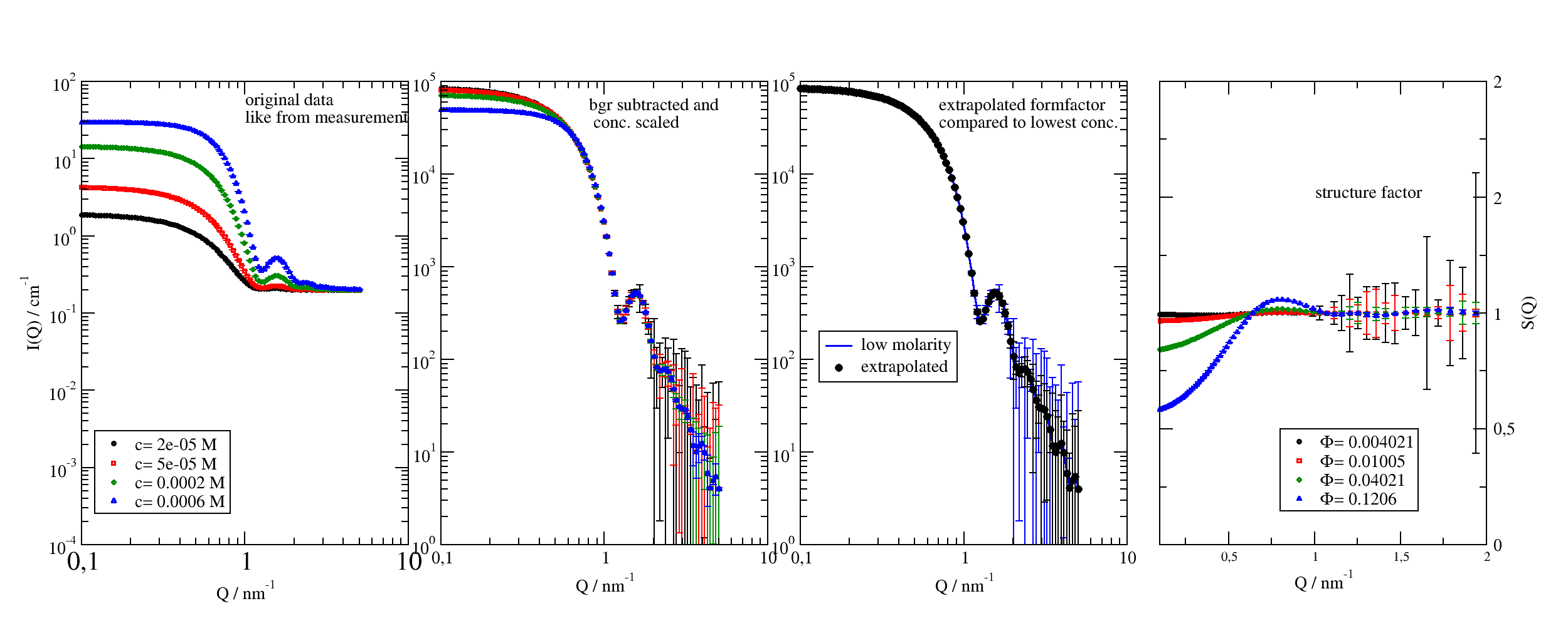
12.5.2. Analysis of SAS data
In small angle scattering a typical situation is that you want to measure a formfactor (particle shape) or structure factor (particle interaction). For this a concentration series is measured and we need to extrapolate to zero concentration to get the formfactor. Afterwards we can divide the measurement by the formfactor to get the structure factor. So we have three key parts :
Correction for transmission, dark and empty cell scattering to get instrument independent datasets.
Extrapolating concentration scaled data to get the formfactor.
Divide by formfactor to get structure factor
Correction
Brulet at al [1]_ describe the data correction for SANS, which is in principle also valid for SAXS, if incoherent contributions are neglected.
The difference is, that SAXS has typical transmission around ~0.3 for 1mm water sample in quartz cell due to absorption, while in SANS typical values are around ~0.9 for D2O. Larger volume fractions in the sample play a more important rule for SANS as hydrogenated ingredients reduce the transmission significantly, while in SAXS still the water and the cell (quartz) dominate.
One finds for a sample inside of a container with thicknesses (\(z\)) for sample, buffer (solvent), empty cell and empty beam measurement (omitting the overall q dependence):
- where
\(I_s\) is the interesting species
\(I_S\) is the sample of species in solvent (buffer)
\(I_B\) is the pure solvent (describing a constant background)
\(I_{dark}\) is the dark current measurement. For Pilatus detectors equal zero.
\(I_b\) is the empty beam measurement
\(I_{EC}\) is the empty cell measurement
\(z_x\) corresponding sample thickness
\(T_x\) corresponding transmission
The recurring pattern \(\big((\frac{I-I_{dark}}{T}-I_{b}T\big)\) shows that the the beam tail (border of primary beam not absorbed by the beam stop) is attenuated by the corresponding sample.
For equal sample thickness \(z\) the empty beam is included in subtraction of \(I_B\) :
The simple case
If the transmissions are nearly equal as for e.g. protein samples with low concentration (\(T_S \approx T_B\)) we only need to subtract the transmission and dark current corrected buffer measurement from the sample.
\[I_s = \frac{1}{z} \big((\frac{I_S-I_{dark}}{T_S}) - (\frac{I_B-I_{dark}}{T_B}\big)\]Higher accuracy for large volume fractions
For larger volume fractions \(\Phi\) the transmission might be different and we have to take into account that only \(1-\Phi\) of solvent contributes to \(I_S\). We may incorporate this in the sense of an optical density changing the effective thickness \(\frac{1}{z_B}\rightarrow\frac{1-\Phi}{z_B}\) resulting in different thicknesses \(z_S \neq z_B\)
Extrapolation and dividing by concentration
We assume that the above correction was correctly applied and we have a transmission corrected sample and buffer (background) measurement. This is what you typically get from SANS instruments as e.g KWS1-3 from MLZ Garching or D11-D33 at ILL, Grenoble.
The key part is dataff=datas.extrapolate(molarity=0)[0] to extrapolate to zero molarity.
# Analyse SAS data by extrapolating the form factor followed by structure factor determination

import jscatter as js
import numpy as np

# generate some synthetic data just for this demonstration
# import the model described in example_buildComplexModel
# it describes ellipsoids with PercusYevick structure factor
from jscatter.examples import particlesWithInteraction as PWI

NN = 100
q = js.loglist(0.1, 5, NN)
data = js.dL()
bgr = js.dA(np.c_[q, 0.2 + np.random.randn(NN) * 1e-3, [1e-3] * NN].T)  # background
for m in [0.02, 0.05, 0.2, 0.6]:
    pwi = PWI(q, Ra=3, Rb=4, molarity=m * 1e-3, bgr=0, contrast=6e-4)
    pwi = pwi.addColumn(1, np.random.randn(NN) * 1e-3)
    pwi.Y = pwi.Y + bgr.Y
    pwi.setColumnIndex(iey=-1)
    data.append(pwi)

# With measured data the above is just reading data and background
# with an attribute molarity or concentration.
# This might look like this
if 0:
    data = js.dL()
    bgr = js.dA('backgroundmeasurement.dat')
    for name in ['data_conc01.dat', 'data_conc02.dat', 'data_conc05.dat', 'data_conc08.dat']:
        data.append(name)
        data[-1].molarity = float(name.split('.')[0][-2:])

p = js.grace(2, 0.8)
p.multi(1, 4)
p[0].plot(data, sy=[-1, 0.3, -1], le='c= $molarity M')
p[0].yaxis(min=1e-4, max=1e2, scale='l', label=r'I(Q) / cm\S-1', tick=[10, 9], charsize=1, ticklabel=['power', 0, 1])
p[0].xaxis(scale='l', label=r'Q / nm\S-1', min=1e-1, max=1e1, charsize=1)
p[0].text(r'original data\nlike from measurement', y=50, x=1)
p[0].legend(x=0.12, y=0.003)

# Using the synthetic data we extract again the form factor and structure factor
# subtract background and scale data by concentration or volume fraction
datas = data.copy()
for dat in datas:
    dat.Y = (dat.Y - bgr.Y) / dat.molarity
    dat.eY = (dat.eY + bgr.eY) / dat.molarity  # errors increase
p[1].plot(datas, sy=[-1, 0.3, -1], le='c= $molarity M')
p[1].yaxis(min=1, max=1e5, scale='l', tick=[10, 9], charsize=1, ticklabel=['power', 0])
p[1].xaxis(scale='l', label=r'Q / nm\S-1', min=1e-1, max=1e1, charsize=1)
p[1].text(r'bgr subtracted and\n conc. scaled', y=5e4, x=0.8)

# extrapolate to zero concentration to get the  form factor
# dataff=datas.extrapolate(molarity=0,func=lambda y:-1/y,invfunc=lambda y:-1/y)
dataff = datas.extrapolate(molarity=0)[0]
# as error *estimate* we may use the mean of the errors which is not absolutely correct
dataff = dataff.addColumn(1, datas.eY.array.mean(axis=0))
dataff.setColumnIndex(iey=2)
p[2].plot(datas[0], li=[1, 2, 4], sy=0, le='low molarity')
p[2].plot(dataff, sy=[1, 0.5, 1, 1], le='extrapolated')
p[2].yaxis(min=1, max=1e5, scale='l', tick=[10, 9], charsize=1, ticklabel=['power', 0])
p[2].xaxis(scale='l', label=r'Q / nm\S-1', min=1e-1, max=1e1, charsize=1)
p[2].legend(x=0.13, y=200)
p[2].text(r'extrapolated formfactor \ncompared to lowest conc.', y=5e4, x=0.7)

# calc the structure factor by dividing by the form factor
sf = datas.copy()
for dat in sf:
    dat.Y = dat.Y / dataff.Y
    dat.eY = (dat.eY ** 2 / dataff.Y ** 2 + dataff.eY ** 2 * (dat.Y / dataff.Y ** 2) ** 2) ** 0.5
    dat.volfrac = dat.Volume * dat.molarity
p[3].plot(sf, sy=[-1, 0.3, -1], le=r'\xF\f{}= $volfrac')
p[3].yaxis(min=0, max=2, scale='n', label=['S(Q)', 1, 'opposite'], charsize=1, ticklabel=['General', 0, 1, 'opposite'])
p[3].xaxis(scale='n', label=r'Q / nm\S-1', min=1e-1, max=2, charsize=1)
p[3].text('structure factor', y=1.5, x=1)
p[3].legend(x=0.8, y=0.5)

# remember so safe the form factor and structurefactor
# sf.save('uniquenamestructurefactor.dat')
# dataff.save('uniquenameformfactor.dat')

# save the figures
p.save('SAS_sf_extraction.agr')
p.save('SAS_sf_extraction.png', size=(2500/300, 1000/300), dpi=300)
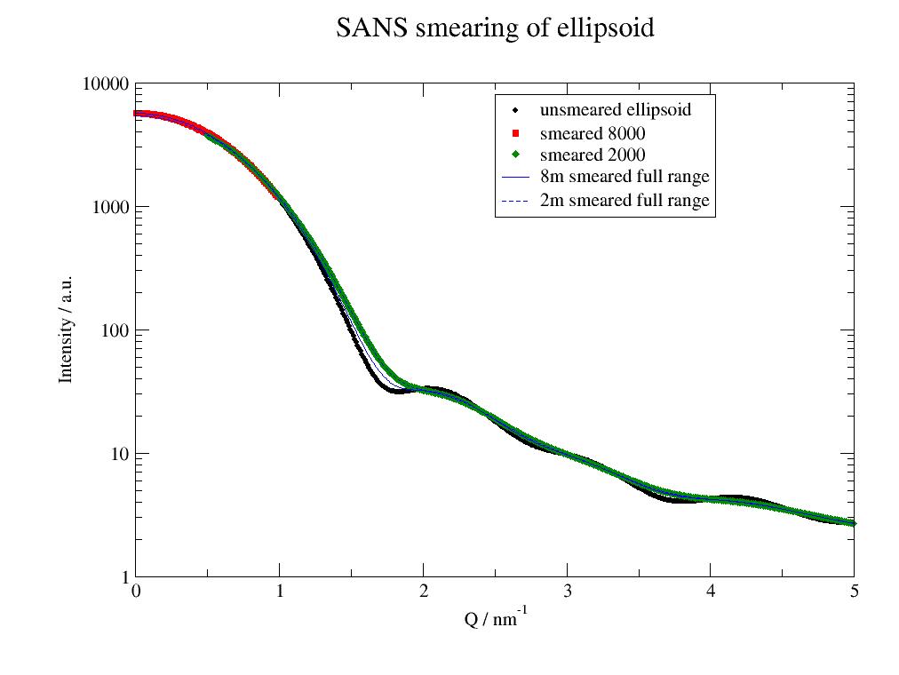
12.5.3. How to fit SANS data including the resolution for different detector distances
- First this example shows the influence of smearing, then how to do a fit including
smearing a la Pedersen. The next example can do the same.
import jscatter as js
import numpy as np

# prepare profiles SANS for typical 2m and 8m measurement
# smear calls resFunc with the respective parameters; smear also works with line collimation SAXS if needed
resol8m = js.sas.prepareBeamProfile('SANS', collDist=8000., collAperture=10, detDist=8000., sampleAperture=10,
                                    wavelength=0.5, wavespread=0.2, dpixelWidth=10, dringwidth=1)


# demonstration smearing effects

# define model and use @smear to wrap it with the smearing function
# detDist and collDist will be used in js.sas.smear to change the beamprofile for smearing

@js.sas.smear(beamProfile=resol8m)
def ellipsoid(q, a, b, bgr, detDist=2000, collDist=2000.):
    elli = js.ff.ellipsoid(q, a, b)
    elli.Y = elli.Y + bgr
    return elli


# generate some smeared data, or load them from measurement
a, b = 2, 3
data = js.dL()
data.append(ellipsoid(np.r_[0.01:1:0.01], a, b, 2, detDist=8000, collDist=8000.))
data.append(ellipsoid(np.r_[0.5:5:0.05], a, b, 2, detDist=2000, collDist=2000.))

# here we compare the difference between the 2 profiles using for both the full q range
data2 = js.dL()
data2.append(ellipsoid(np.r_[0.01:5:0.02], a, b, 2, detDist=8000, collDist=8000.))
data2.append(ellipsoid(np.r_[0.01:5:0.02], a, b, 2, detDist=2000, collDist=2000.))

# plot it
p = js.grace()
ellip = js.ff.ellipsoid(np.r_[0.01:5:0.01], a, b)
ellip.Y += 2
p.plot(ellip, sy=[1, 0.3, 1], legend='unsmeared ellipsoid')
p.yaxis(label='Intensity / a.u.', scale='l', min=1, max=1e4)
p.xaxis(label=r'Q / nm\S-1', scale='n')
p.plot(data, legend='smeared $rf_detDist')
p.plot(data2[0], li=[1, 1, 4], sy=0, legend='8m smeared full range')
p.plot(data2[1], li=[3, 1, 4], sy=0, legend='2m smeared full range')
p.legend(x=2.5, y=8000)
p.title('SANS smearing of ellipsoid')
p.save('SANSsmearing.jpg')

# now we use the simulated data to fit this to a model
# the data need attributes detDist and collDist to use correct parameters in smearing
# here we add these from above in rf_detDist (set in smear)
# for a measurement this needs to be added to the experimental data
data[0].detDist = data[0].rf_detDist
data[0].collDist = data[0].rf_collDist
data[1].detDist = data[1].rf_detDist
data[1].collDist = data[1].rf_collDist


@js.sas.smear(beamProfile=resol8m)
def smearedellipsoid(q, A, a, b, bgr, detDist=2000, collDist=2000.):
    """
    The model may use all needed parameters for smearing.
    """
    ff = js.ff.ellipsoid(q, a, b)  # calc model
    ff.Y = ff.Y * A + bgr  # multiply amplitude factor and add bgr
    return ff


# fit it , here no errors
data.makeErrPlot(yscale='l', fitlinecolor=[1, 2, 5])
data.fit(smearedellipsoid, {'A': 1, 'a': 2.5, 'b': 3.5, 'bgr': 0}, {}, {'q': 'X'})
# show the unsmeared model
p = js.grace()
for oo in data:
    p.plot(oo, sy=[-1, 0.5, -1], le='lastfit smeared')
    p.plot(oo.X, oo[2], li=[3, 2, 4], sy=0, legend='lastfit unsmeared')
p.yaxis(scale='l')
p.legend()
p.save('SANSsmearingFit.jpg')
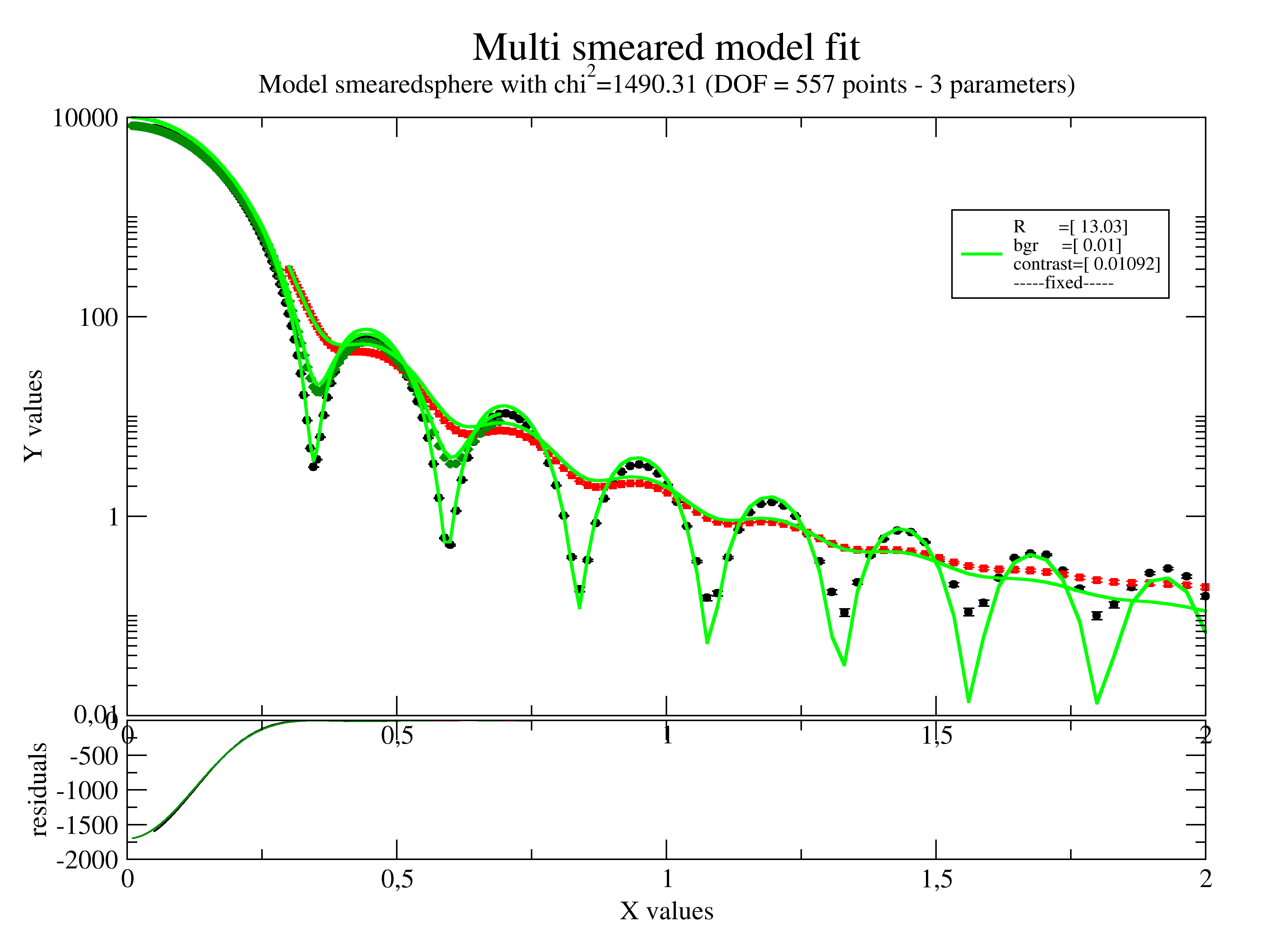
12.5.4. Fitting multiple smeared data together
In the following example all smearing types may be mixed and can be fitted together.
For details and more examples on smearing see smear()
This examples shows SAXS/SANS smearing with different collimation.
import jscatter as js
import numpy as np

# prepare beamprofiles according to measurement setup
# SAXS with small resolution
fbeam = js.sas.prepareBeamProfile(0.01)
# low and high Q SANS
Sbeam4m = js.sas.prepareBeamProfile('SANS', detDist=4000, wavelength=0.4, wavespread=0.1)
Sbeam20m = js.sas.prepareBeamProfile('SANS', detDist=20000, wavelength=0.4, wavespread=0.1)


# define smeared model with beamProfile as parameter
@js.sas.smear(beamProfile=fbeam)
def smearedsphere(q, R, bgr, contrast=1, beamProfile=None):
    sp = js.ff.sphere(q=q, radius=R, contrast=contrast)
    sp.Y = sp.Y + bgr
    return sp


# read data with 3 measurements
smeared = js.dL(js.examples.datapath+'/smearedSASdata.dat')

# add corresponding smearing to the datasets
# that the model can see in attribute beamprofile how to smear
smeared[0].beamProfile = fbeam
smeared[1].beamProfile = Sbeam4m
smeared[2].beamProfile = Sbeam20m

if 0:
    # For scattering data it is sometimes advantageous
    # to use a log weight in fit using the error weight
    for temp in smeared:
        temp.eY = temp.eY *np.log(temp.Y)

# fit it
smeared.setlimit(bgr=[0.01])
smeared.makeErrPlot(yscale='l', fitlinecolor=[1, 2, 5], title='Multi smeared model fit')
smeared.fit(smearedsphere, {'R': 12, 'bgr': 0.1, 'contrast': 1e-2}, {}, {'q': 'X'})
# smeared.errplot.save(js.examples.imagepath+'/smearedfitexample.png')
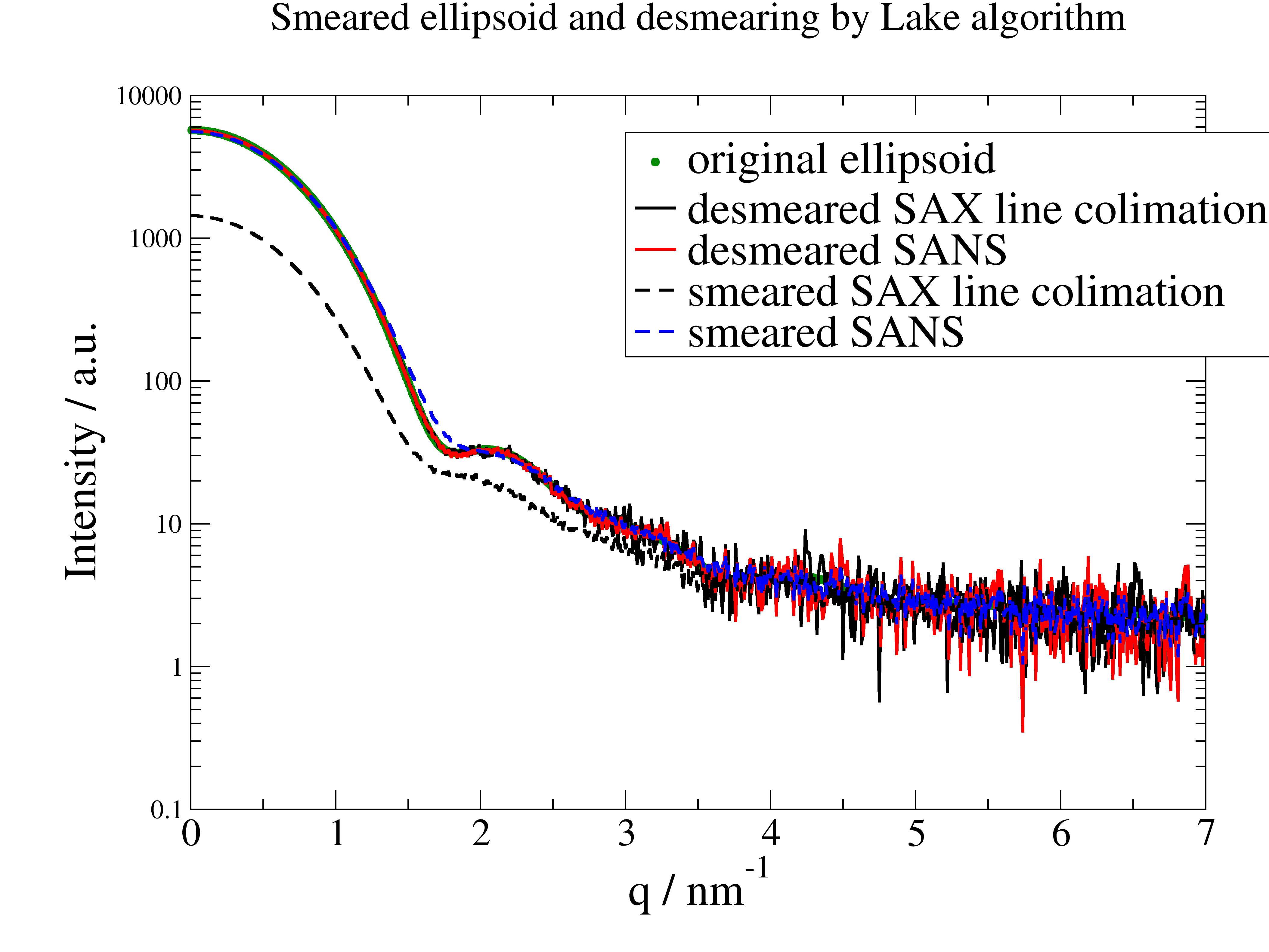
12.5.5. Smearing and desmearing of SAX and SANS data
Here we examine the effect of instrumental smearing for SAX (Kratky Camera, line! ) and SANS and how we can use the Lake algorithm for desmearing.
The conclusion is that because of the increased noise it is in most cases more effective to fit smeared models than to desmear data and fit these. The additional advantage is that at the edges (eg detector limits) we can desmear a model correctly while we need assumptions for the data (e.g. low Q Guinier behavior, high Q as constant) which are sometimes difficult to justify.
import jscatter as js
import numpy as np

# Here we examine the effect of instrumental smearing for SAX (Kratky Camera, line! ) and SANS
# and how we can use the Lake algorithm for desmearing.

# some data
q = np.r_[0.01:7:0.01]
# obj = js.ff.sphere(q,5)
data = js.ff.ellipsoid(q, 2, 3)
# add background
data.Y += 2
# load data for beam width profile
empty = js.dA(js.examples.datapath + '/buffer_averaged_corrected_despiked.pdh', usecols=[0, 1],
              lines2parameter=[2, 3, 4])
# read beam length profile measurement for a slit (Kratky Camera)
beam = js.dA(js.examples.datapath + '/BeamProfile.pdh', usecols=[0, 1], lines2parameter=[2, 3, 4])

# fit beam width for line collimation with semitransparent beam stop
bwidth = js.sas.getBeamWidth(empty, 'auto')

# prepare measured beamprofile from beam measurement
mbeam = js.sas.prepareBeamProfile(beam, a=2, b=1, bxw=bwidth, dIW=1.)
# prepare profile with trapezoidal shape using explicit given parameters (using parameters from above to have equal)
tbeam = js.sas.prepareBeamProfile('trapez', a=mbeam.a, b=mbeam.b, bxw=bwidth, dIW=1)
# prepare profile SANS a la Pedersen in point collimation. This can be used for SAXS with smaller apertures too!
Sbeam = js.sas.prepareBeamProfile('SANS', detDist=2000, wavelength=0.4, wavespread=0.15)

if 0:
    p = js.sas.plotBeamProfile(mbeam)
    p = js.sas.plotBeamProfile(mbeam, p)

# smear
datasm = js.sas.smear(unsmeared=data, beamProfile=mbeam)
datast = js.sas.smear(unsmeared=data, beamProfile=tbeam)
datasS = js.sas.smear(unsmeared=data, beamProfile=Sbeam)
# add noise
datasm.Y += np.random.normal(0, 0.5, len(datasm.X))
datast.Y += np.random.normal(0, 0.5, len(datast.X))
datasS.Y += np.random.normal(0, 0.5, len(datasS.X))

# desmear again
ws = 11
NI = -15
dsm = js.sas.desmear(datasm, mbeam, NIterations=NI, windowsize=ws)
dst = js.sas.desmear(datast, tbeam, NIterations=NI, windowsize=ws)
dsS = js.sas.desmear(datasS, Sbeam, NIterations=NI, windowsize=ws)

# compare
p = js.grace(2, 1.4)
p.plot(data, sy=[1, 0.3, 3], le='original ellipsoid')
p.plot(dst, sy=0, li=[1, 2, 1], le='desmeared SAX line collimation')
p.plot(dsS, sy=0, li=[1, 2, 2], le='desmeared SANS')
p.plot(datasm, li=[3, 2, 1], sy=0, le='smeared SAX line collimation')
p.plot(datasS, li=[3, 2, 4], sy=0, le='smeared SANS')
p.yaxis(max=1e4, min=0.1, scale='l', label='Intensity / a.u.', size=1.7)
p.xaxis(label=r'q / nm\S-1', size=1.7)
p.legend(x=3, y=5500, charsize=1.7)
p.title('Smeared ellipsoid and desmearing by Lake algorithm')

# The conclusion is to better fit smeared models than to desmear and fit unsmeared models.
p.save('SASdesmearing.png')
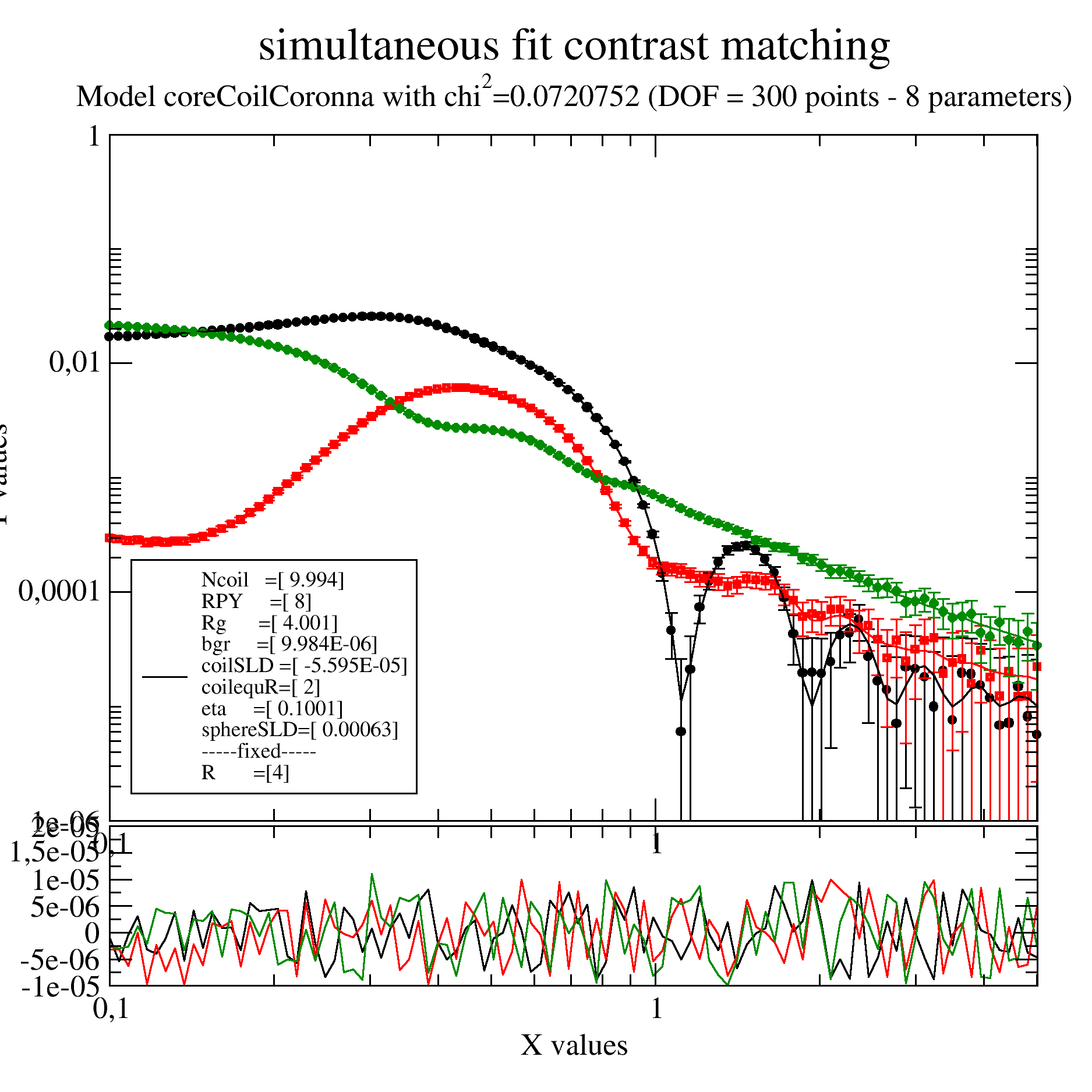
12.5.6. Simultaneous fit SANS data of a partly matched sample measured at 3 contrast conditions
In this example we ignore smearing (Add it if needed).
We have a sample like a micelles of a diblock copolymer with a shorter hydrophobic and a longer hydrophilic part. The hydrophobic part will make a core with hydrophilic extended Gaussian coils into the solvent.
To separate core and coils 3 contrast were measured in H2O, a H2O/D2O mixture with SLD 3e-4 and D2O.
As a reasonable high concentration was used we observe in the core contrast (black points) already a structure factor as a maximum at around 0.3 /nm. The minimum around 1 /nm defines the core radius in ths contrast that we fix. This structure factor we need to include.
We do a simultaneous fit of all together using the coreGaussiancoronna model. To add structure factor and background we write our own model.
import jscatter as js

# read data measured at 3 contrast conditions:
i5 = js.dL(js.examples.datapath + '/gauscoronna.dat')
# add solvent contrast to data from preparation, will be used as fixed parameter per dataArray
i5[0].solventSLD = -0.56e-4    # H2O contrast (nearly its actually lower, but this is just an example)
i5[1].solventSLD = 3e-4        # some H2O/D2O mixture
i5[2].solventSLD = 6.3e-4      # D2O
i5.setlimit(bgr=[0, 0.00001], RPY=[0, 20])


# define sphereGaussianCorona with background
def coreCoilCoronna(q, R, Ncoil, Nmonomer, monomerVolume, a, coilSLD, sphereSLD, solventSLD, RPY,eta,bgr):
    res = js.ff.sphereGaussianCorona(q, R=R, Ncoil=Ncoil,Nmonomer=Nmonomer,monomerVolume=monomerVolume,a=a ,
                                     coilSLD=coilSLD, sphereSLD=sphereSLD, solventSLD=solventSLD)
    res.Y =res.Y * js.sf.PercusYevick(q, RPY, eta=eta).Y + bgr
    return res


# make ErrPlot to see progress of intermediate steps with residuals (updated all 2 seconds)
i5.makeErrPlot(title='simultaneous fit contrast matching', xscale='log', yscale='log', legpos=[0.12, 0.5])

# fit it
# the minimum in core contrast can be used to predetermine "R":4
# Method 'Nelder-Mead' searches more for a solution,direct use of 'lm' works here
i5.fit(model=coreCoilCoronna,  # the fit function
       freepar={ 'Ncoil': 8, 'Nmonomer':100,
                 'coilSLD': 3e-4, 'sphereSLD': 3e-4, 'bgr': 0, 'RPY':7,'eta':0.1},
       fixpar={'R': 4, 'a':0.8, 'monomerVolume':0.12},
       mapNames={'q': 'X', })

# use a 'lm' to polish the result and get errors using the last fit result as start
# here this really improves the fit
i5.estimateError()

# i5.errplot.save(js.examples.imagepath+'/multicontrastfit.png', size=(1.5, 1.5))
12.5.7. Multilamellar Vesicles
Here we look at the various effects appearing for vesicles and how they change the scattering.
import jscatter as js

Q = js.loglist(0.001, 5, 500)  # np.r_[0.01:5:0.01]

ffmV = js.ff.multilamellarVesicles
save = 0

# correlation peak sharpness depends on disorder
dR = 20
nG = 200
p = js.grace(1, 1)
for dd in [0.1, 6, 10]:
    p.plot(ffmV(Q=Q, R=100, displace=dd, dR=dR, N=10, dN=0, phi=0.2, nGauss=nG),
           le='displace= %g ' % dd)

p.legend(x=0.3, y=10)
p.title('Scattering of multilamellar vesicle')
p.subtitle('lamella N=10, layerd 0 nm, dR=20, R=100')
p.yaxis(label='S(Q)', scale='l', min=1e-7, max=1e2, ticklabel=['power', 0])
p.xaxis(label=r'Q / nm\S-1', scale='l', min=1e-3, max=5, ticklabel=['power', 0])
p.text('Guinier range', x=0.005, y=10)
p.text(r'Correlation peaks\nsharpness decreases with disorder', x=0.02, y=0.00001)
if save: p.save('multilamellar1.png')

# Correlation peak position depends on average layer distance
dd = 0
dR = 20
nG = 200
p = js.grace(1, 1)
for N in [1, 3, 10, 30, 100]:
    p.plot(ffmV(Q=Q, R=100, displace=dd, dR=dR, N=N, dN=0, phi=0.2, nGauss=nG), le='N= %g ' % N)

p.legend(x=0.3, y=10)
p.title('Scattering of multilamellar vesicle')
p.subtitle('shellnumber N, layers 0 nm, dR=20, R=100')
p.yaxis(label='S(Q)', scale='l', min=1e-7, max=1e2, ticklabel=['power', 0])
p.xaxis(label=r'Q / nm\S-1', scale='l', min=1e-3, max=5, ticklabel=['power', 0])

p.text('Guinier range', x=0.005, y=40)
p.text(r'Correlation peaks\n at 2\xp\f{}N/R', x=0.2, y=0.01)
if save: p.save('multilamellar2.png')

# including the shell formfactor with fluctuations of layer thickness
dd = 2
dR = 20
nG = 200
p = js.grace(1, 1)
# multi lamellar structure factor
mV = ffmV(Q=Q, R=100, displace=dd, dR=dR, N=10, dN=0, phi=0.2, layerd=6, layerSLD=1e-4, nGauss=nG)
for i, ds in enumerate([0.001, 0.1, 0.6, 1.2], 1):
    # calc layer fomfactor
    lf = js.formel.pDA(js.ff.multilayer, ds, 'layerd', q=Q, layerd=6, layerSLD=1e-4)
    p.plot(mV.X, mV._Sq * lf.Y / lf.Y[0], sy=[i, 0.3, i], le='ds= %g ' % ds)
    p.plot(mV.X, lf.Y, sy=0, li=[3, 3, i])
    p.plot(mV.X, mV._Sq, sy=0, li=[2, 3, i])

p.legend(x=0.003, y=1)
p.title('Scattering of multilamellar vesicle')
p.subtitle('shellnumber N=10, layers 6 nm, dR=20, R=100')
p.yaxis(label='S(Q)', scale='l', min=1e-12, max=1e2, ticklabel=['power', 0])
p.xaxis(label=r'Q / nm\S-1', scale='l', min=2e-3, max=5, ticklabel=['power', 0])

p.text('Guinier range', x=0.005, y=10)
p.text(r'Correlation peak\n at 2\xp\f{}N/R', x=0.4, y=5e-3)
p.text('Shell form factor', x=0.03, y=1e-6)
p.text(r'Shell structure factor', x=0.02, y=2e-5)
p[0].line(0.08, 1e-5, 2, 1e-5, 2, arrow=2)
if save: p.save('multilamellar3.png')

# Comparing multilamellar and unilamellar vesicle
dd = 2
dR = 5
nG = 100
ds = 0.2
N = 4
p = js.grace(1, 1)
for i, R in enumerate([40, 50, 60], 1):
    mV = ffmV(Q=Q, R=R, displace=dd, dR=dR, N=N, dN=0, phi=0.2, layerd=6, ds=ds, layerSLD=1e-4, nGauss=nG)
    p.plot(mV, sy=[i, 0.3, i], le='R= %g ' % R)
    p.plot(mV.X, mV[-2] * 0.01, sy=0, li=[1, 1, i])
# is same for all
p.plot(mV.X, mV[-1], sy=0, li=[1, 1, 1])

# comparison double sphere
mV = ffmV(Q=Q, R=50., displace=0, dR=5, N=1, dN=0, phi=1, layerd=6, ds=ds, layerSLD=1e-4, nGauss=100)
p.plot(mV, sy=0, li=[1, 2, 4], le='unilamellar R=50 nm')
mV = ffmV(Q=Q, R=60., displace=0, dR=5, N=1, dN=0, phi=1, layerd=6, ds=ds, layerSLD=1e-4, nGauss=100)
p.plot(mV, sy=0, li=[3, 2, 4], le='unilamellar R=60 nm')

p.legend(x=0.3, y=2e3)
p.title('Comparing multilamellar and unilamellar vesicle')
p.subtitle(f'R={R} nm, N={N}, layers={6} nm, dR={dR}, ds={ds}')
p.yaxis(label='S(Q)', scale='l', min=1e-10, max=1e4, ticklabel=['power', 0])
p.xaxis(label=r'Q / nm\S-1', scale='l', min=1e-2, max=5, ticklabel=['power', 0])

p.text('Guinier range', x=0.02, y=1000)
p.text(r'Correlation peaks\n at 2\xp\f{}N/R', x=0.8, y=0.1)
p[0].line(0.8, 4e-2, 0.6, 4e-2, 2, arrow=2)
p.text('Shell form factor', x=1.3, y=0.3e-2, rot=335)
# p[0].line(0.2,4e-5,0.8,4e-5,2,arrow=2)
p.text(r'Shell structure factor\n x0.01', x=0.011, y=0.1, rot=0)
p.text('Shell form factor ', x=0.02, y=2e-6, rot=0)
if save: p.save('multilamellar4.png')
The first image shows how a multilamellar vesicles changes the shape of the membrane correlation peak with increasing dislocations of the centers.
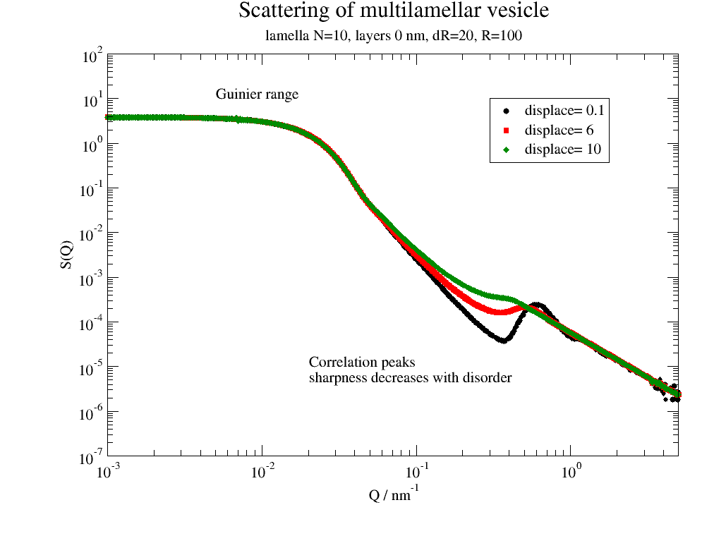
Larger number of lamella shifts the correlation peak to higher Q.
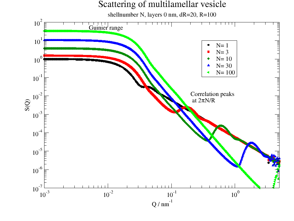
The shell formfactor determines the high Q minima. This allows to access the structure of e.g. bilayers.
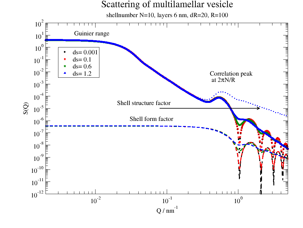
Multilamellar and unilamellar can be distinguished with the aid of the appearing correlation peaks. See below.
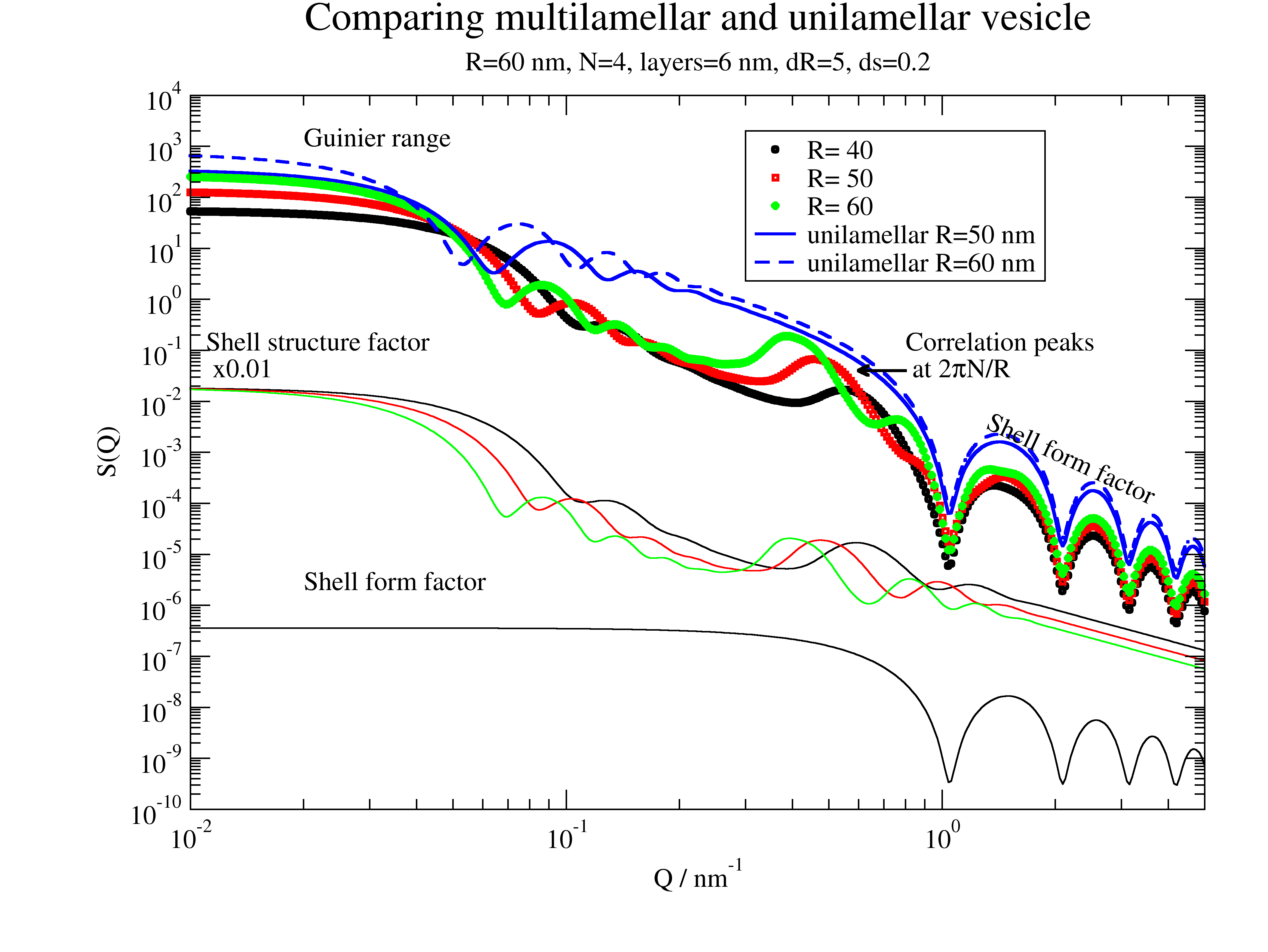
12.5.8. DPPC Vesicle in SAXS
A more realistic example for DPPC We use a simplified model with 3 box layers and approximate thickness and scattering length densities. Kučerka uses a multi Gaussian profile.
# Values for layer thickness can be found in
# Structure of lipid bilayers
# John F. Nagle et al. Biochim Biophys Acta. 1469, 159–195. (2000)

# scattering length densities of head groups and tails
# Small-Angle Neutron Scattering for Studying Lipid Bilayer Membranes
# William T Heller, Biomolecules 2022 Oct 29;12(11):1591.   doi: 10.3390/biom12111591.
#
# phospholipid headgroups (HG) in 1e-4 nm^2
# PC HG           1.877
# 2H18-PC HG      7.736
# PE HG           2.483
# PA HG           2.494
# PG HG (in H2O)  2.382
# PG HG (in2H2O)  3.076
# PS HG (in H2O)  3.466
# PS HG (in2H2O)  3.893
#
# acyl chains in phospholipids in 1e-4 nm^2
# lauroyl (12:0)         -0.386
# 2H23-lauroyl (12:0)     6.755
# myristoyl (14:0)       -0.375
# 2H27-myristoyl (14:0)   6.837
# palmitoyl (16:0)       -0.386
# 2H31-palmitoyl (16:0)   6.557
# oleoyl (18:1c)         -0.386
#
# cholesterol (in H2O)    0.216
# cholesterol (in2H2O)    0.386


import jscatter as js
import numpy as np

ffmV = js.ff.multilamellarVesicles
save = 0

Q = js.loglist(0.01, 7, 500)
dd = 1.5
dR = 5
nG = 100
ds = 0.05  # variation of hydrocarbon layer thickness
R = 50
sd = [0.75, 2.8, 0.75]
N = 2

p = js.grace(1.4,1)
p.title('Multilamellar/unilamellar vesicle for SAXS/SANS')
# SAXS
sld = np.r_[420, 290, 420] * js.formel.felectron  # unit e/nm³*fe
sSLD = 335 * js.formel.felectron  # H2O unit e/nm³*fe
saxm = ffmV(Q=Q, R=R, displace=dd, dR=dR, N=N, dN=0, phi=0.2, layerd=sd, ds=ds, layerSLD=sld, solventSLD=sSLD, nGauss=nG)
p.plot(saxm, sy=0, li=[1, 1, 1], le='multilamellar')
saxu = ffmV(Q=Q, R=R, displace=0, dR=dR, N=1, dN=0, phi=0.2, layerd=sd, ds=ds, layerSLD=sld, solventSLD=sSLD, nGauss=100)
p.plot(saxu, sy=0, li=[3, 2, 1], le='unilamellar')
saxu0 = ffmV(Q=Q, R=R, displace=0, dR=dR, N=1, dN=0, phi=0.2, layerd=sd, ds=0, layerSLD=sld, solventSLD=sSLD, nGauss=100)
p.plot(saxu0, sy=0, li=[2, 0.3, 1], le='unilamellar ds=0')
p.text('SAXS', x=0.015, y=0.2, charsize=1.5,color=1)

# SANS
sld = [1.877e-4, -.375e-4, 1.877e-4]  # unit 1/nm²
sSLD = 6.335e-4  # D2O
sanm = ffmV(Q=Q, R=R, displace=dd, dR=dR, N=N, dN=0, phi=0.2, layerd=sd, ds=ds, layerSLD=sld, solventSLD=sSLD, nGauss=nG)
p.plot(sanm, sy=0, li=[1, 1, 2], le='multilamellar')
sanu = ffmV(Q=Q, R=R, displace=0, dR=dR, N=1, dN=0, phi=0.2, layerd=sd, ds=ds, layerSLD=sld, solventSLD=sSLD, nGauss=100)
p.plot(sanu, sy=0, li=[3, 2, 2], le='unilamellar')
sanu = ffmV(Q=Q, R=R, displace=0, dR=dR, N=1, dN=0, phi=0.2, layerd=sd, ds=0, layerSLD=sld, solventSLD=sSLD, nGauss=100)
p.plot(sanu, sy=0, li=[2, 0.3, 2], le='unilamellar ds=0')
p.text('SANS', x=0.015, y=50, charsize=1.5,color=2)

p.legend(x=0.8, y=950, boxcolor=0, boxfillpattern=0)
p.subtitle('R=%.2g nm, N=%.1g, layerd=%s nm, dR=%.1g, ds=%.2g' % (R, N, sd, dR, ds))

p.yaxis(label='S(Q)', scale='l', min=2e-6, max=2e3, ticklabel=['power', 0])
p.xaxis(label=r'Q / nm\S-1', scale='l', min=1e-2, max=9, ticklabel=['power', 0])
p.text(r'Correlation peaks\n at 2\xp\f{}N/R', x=0.25, y=0.05, charsize=1.,color=1)
p.text('Guinier range', x=0.03, y=900, charsize=1.)
p.text('Shell form factor ds=0', x=0.2, y=0.2e-4)
p[0].line(0.3, 1e-5, 1.3, 1e-5, 2, arrow=2)
if save: p.save('multilamellar5.png')
We observe in this figure modulations at the left flank of the prominent peak. The modulations are caused by the multilamelarity and a clear indication. Already small modulations indicate multi lamellar vesicles in accordance with Kučerka et al.
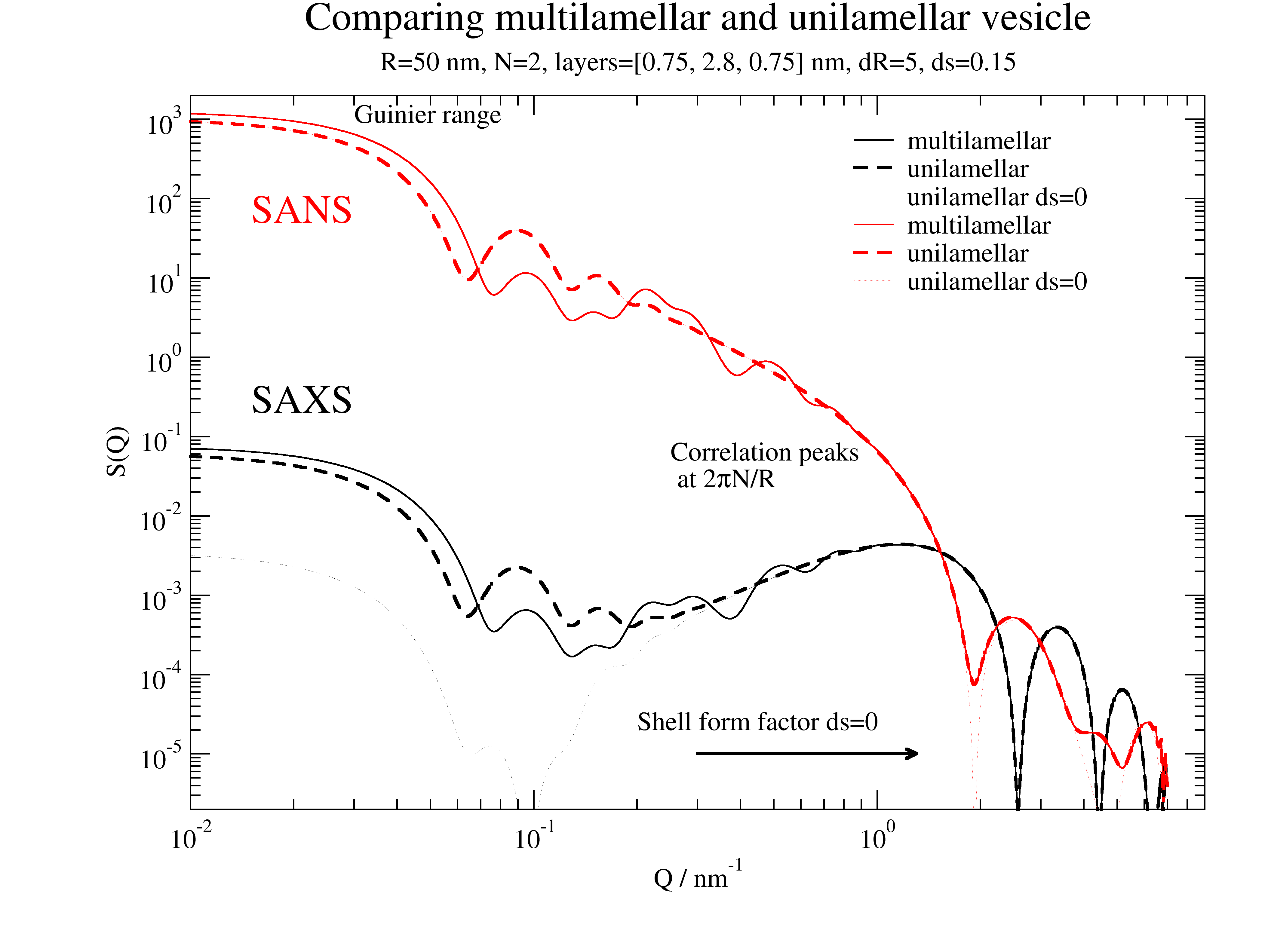
Multilamellar SAXS example for DPPC
The first minima with following increase is a result of the near matching condition for bilayers in SAXS. Additionally we observe characteristic peaks/shoulders in the first increase/top as a result of multilamellar interference. See for comparison Kučerka et al. Langmuir 23, 1292 (2007) https://doi.org/10.1021/la062455t .
We use again the simplified model with 3 box layers and approximate thickness from above
# Values for layer thickness can be found in
# Structure of lipid bilayers
# John F. Nagle et al.Biochim Biophys Acta. 1469, 159–195. (2000)

# scattering length densities of DPPC for SAXS and SANS can be found in
#  Kučerka et al. Biophysical Journal. 95,2356 (2008)
#  https://doi.org/10.1529/biophysj.108.132662

import jscatter as js
import numpy as np

ffmV = js.ff.multilamellarVesicles
save = 0

Q = js.loglist(0.01, 7, 500)
dd = 1.5
dR = 5
nG = 100
ds = 0.05  # variation of hydrocarbon layer thickness
R = 50
sd = [0.75, 2.8, 0.75]
N = 2

p = js.grace(1.4,1)
p.title('Multilamellar/unilamellar vesicle for SAXS/SANS')

# SAXS
sld = np.r_[420, 290, 420] * js.formel.felectron  # unit e/nm³*fe
sSLD = 335 * js.formel.felectron  # H2O unit e/nm³*fe
saxu = ffmV(Q=Q, R=R, displace=0, dR=dR, N=1, dN=0, phi=0.2, layerd=sd, ds=ds, layerSLD=sld, solventSLD=sSLD, nGauss=100)
saxu0 = ffmV(Q=Q, R=R, displace=0, dR=dR, N=1, dN=0, phi=0.2, layerd=sd, ds=0, layerSLD=sld, solventSLD=sSLD, nGauss=100)

p.plot(saxu, sy=0, li=[1, 3, 3], le='unilamellar')
p.plot(saxu0, sy=0, li=[2, 0.3, 1], le='unilamellar ds=0')
N=2; dN=0; dR=5
saxm = ffmV(Q=Q, R=R, displace=dd, dR=dR, N=N, dN=0, phi=0.2, layerd=sd, ds=ds, layerSLD=sld, solventSLD=sSLD, nGauss=nG)
p.plot(saxm, sy=0, li=[1, 1, 1], le=f'multilamellar N={N} dN={dN} dR={dR}')
N=3; dN=1; dR=6
saxm = ffmV(Q=Q, R=R, displace=dd, dR=dR, N=N, dN=dN, phi=0.2, layerd=sd, ds=ds, layerSLD=sld, solventSLD=sSLD, nGauss=nG)
p.plot(saxm, sy=0, li=[1, 3, 4], le=f'multilamellar N={N} dN={dN} dR={dR}')


p.legend(x=3, y=0.004, boxcolor=0, boxfillpattern=0)
p.subtitle('R=%.2g nm, layers=%s nm, dR=%.1g, ds=%.2g' % (R, sd, dR, ds))
p.yaxis(label='S(Q)', scale='n', min=0.0, max=5e-3)
p.xaxis(label=r'Q / nm\S-1', scale='n', min=0, max=6)
p.text(r'correlation peaks\n at 2\xp\f{}N/R', x=2, y=0.003, charsize=1., color=1)
p[0].line(0.77,0.0023,2,2.7e-3, 3,1,1,1,2,2)
p[0].line(1.2,0.0042,2,3.3e-3, 3,1,1,1,2,2)
p.text(r'minima due to matching', x=0.3, y=0.002, charsize=1.3, rot=90)

if save: p.save('multilamellar5SAXS.png')
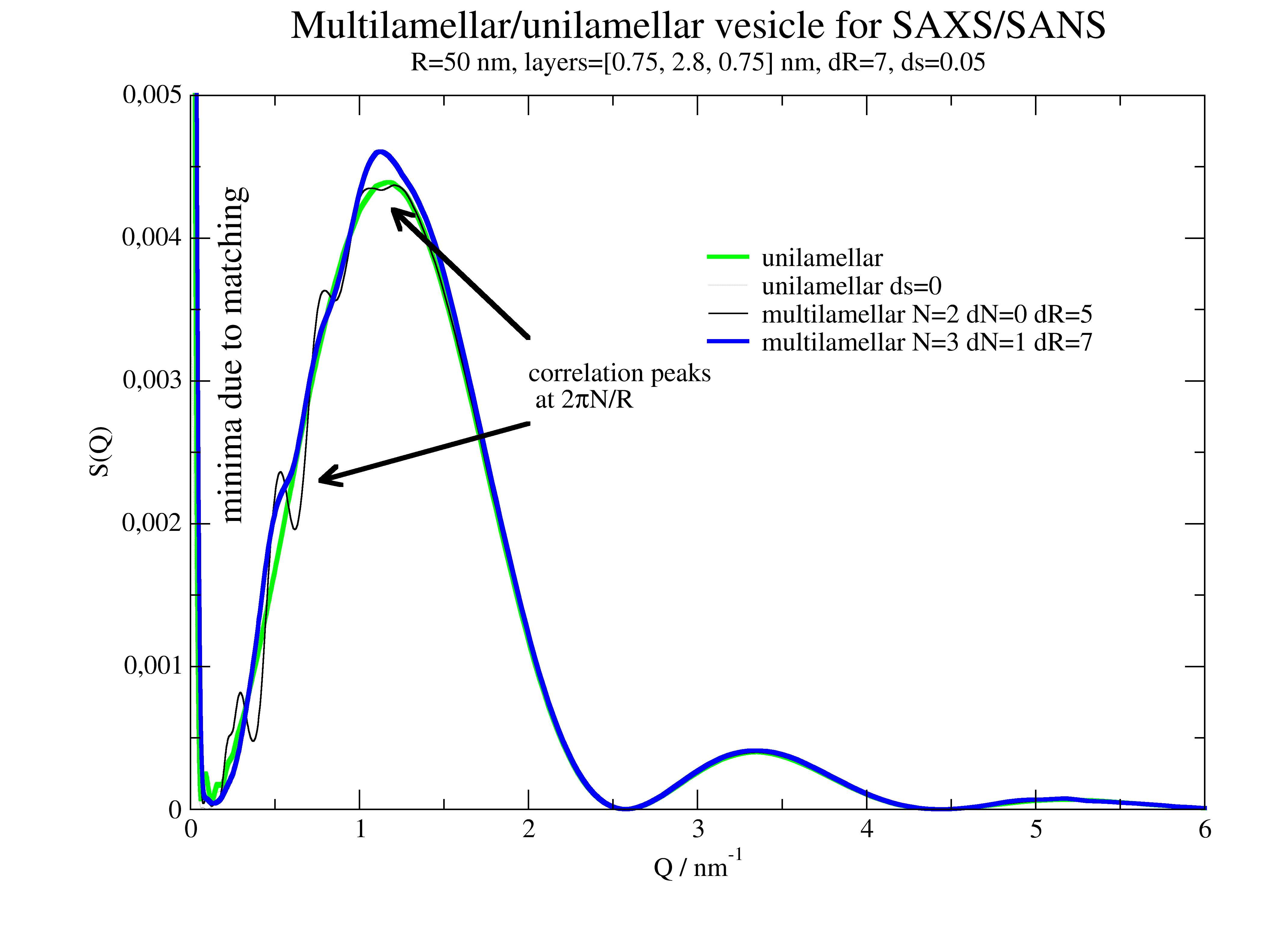
12.5.9. 2D oriented scattering
Formfactors of oriented particles or particle complexes
import jscatter as js
import numpy as np

# Examples for scattering of 2D scattering of some spheres oriented in space relative to incoming beam
# incoming beam along Y
# detector plane X,Z
# For latter possibility to fit 2D data we have Y=f(X,Z)

# two points
rod0 = np.zeros([2, 3])
rod0[:, 1] = np.r_[0, np.pi]
qxz = np.mgrid[-6:6:50j, -6:6:50j].reshape(2, -1).T
ffe = js.ff.orientedCloudScattering(qxz, rod0, mosaicity=[10,0,0], nCone=10, rms=0)
fig = js.mpl.surface(ffe.X, ffe.Z, ffe.Y)
fig.axes[0].set_title('cos**2 for Z and slow decay for X')
fig.show()
# noise in positions
ffe = js.ff.orientedCloudScattering(qxz, rod0, mosaicity=[10,0,0], nCone=100, rms=0.1)
fig = js.mpl.surface(ffe.X, ffe.Z, ffe.Y)
fig.axes[0].set_title('cos**2 for Y and slow decay for X with position noise')
fig.show()
#
# two points along z result in symmetric pattern around zero
# asymmetry is due to small nCone and reflects the used Fibonacci lattice
rod0 = np.zeros([2, 3])
rod0[:, 2] = np.r_[0, np.pi]
ffe = js.ff.orientedCloudScattering(qxz, rod0, mosaicity=[45,0,0], nCone=10, rms=0.05)
fig2 = js.mpl.surface(ffe.X, ffe.Z, ffe.Y)
fig2.axes[0].set_title('symmetric around zero')
fig2.show()
#
# 5 spheres in line with small position distortion
rod0 = np.zeros([5, 3])
rod0[:, 1] = np.r_[0, 1, 2, 3, 4] * 3
qxz = np.mgrid[-6:6:50j, -6:6:50j].reshape(2, -1).T
ffe = js.ff.orientedCloudScattering(qxz, rod0, formfactoramp='sphere', V=4 / 3. * np.pi * 2 ** 3, mosaicity=[20,0,0],
                                    nCone=30, rms=0.02)
fig4 = js.mpl.surface(ffe.X, ffe.Z, np.log10(ffe.Y), colorMap='gnuplot')
fig4.axes[0].set_title('5 spheres with R=2 along Z with noise (rms=0.02)')
fig4.show()
#
# 5 core shell particles in line with small position distortion (Gaussian)
rod0 = np.zeros([5, 3])
rod0[:, 1] = np.r_[0, 1, 2, 3, 4] * 3
qxz = np.mgrid[-6:6:50j, -6:6:50j].reshape(2, -1).T
# only as demo : extract q from qxz
qxzy = np.c_[qxz, np.zeros_like(qxz[:, 0])]
qrpt = js.formel.xyz2rphitheta(qxzy)
q = np.unique(sorted(qrpt[:, 0]))
# or use interpolation
q = js.loglist(0.01, 7, 100)
# explicitly given isotropic form factor amplitude
cs = js.ff.sphereCoreShell(q=q, Rc=1, Rs=2, bc=0.1, bs=1, solventSLD=0)[[0, 2]]
ffe = js.ff.orientedCloudScattering(qxz, rod0, formfactoramp=cs, mosaicity=[20,0,0], nCone=100, rms=0.05)
fig4 = js.mpl.surface(ffe.X, ffe.Z, np.log10(ffe.Y), colorMap='gnuplot')
fig4.axes[0].set_title('5 core shell particles with R=2 along Z with noise (rms=0.05)')
fig4.show()

# Extracting 1D data
# 1. average angular region (similar to experimental detector data)
# 2. direct calculation
# Here with higher resolution to see the additional peaks due to alignment.
#
# 1:
rod0 = np.zeros([5, 3])
rod0[:, 1] = np.r_[0, 1, 2, 3, 4] * 3
qxz = np.mgrid[-4:4:150j, -4:4:150j].reshape(2, -1).T
# only as demo : extract q from qxz
qxzy = np.c_[qxz, np.zeros_like(qxz[:, 0])]
qrpt = js.formel.xyz2rphitheta(qxzy)
q = np.unique(sorted(qrpt[:, 0]))
# or use interpolation
q = js.loglist(0.01, 7, 100)
cs = js.ff.sphereCoreShell(q=q, Rc=1, Rs=2, bc=0.1, bs=1, solventSLD=0)[[0, 2]]
ffe = js.ff.orientedCloudScattering(qxz, rod0, formfactoramp=cs, mosaicity=[20,0,0], nCone=100, rms=0.05)
fig4 = js.mpl.surface(ffe.X, ffe.Z, np.log10(ffe.Y), colorMap='gnuplot')
fig4.axes[0].set_title('5 core shell particles with R=2 along Z with noise (rms=0.05)')
fig4.show()
#
# transform X,Z to spherical coordinates
qphi = js.formel.xyz2rphitheta([ffe.X, ffe.Z, abs(ffe.X * 0)], transpose=True)[:, :2]
# add qphi or use later rp[1] for selection
ffb = ffe.addColumn(2, qphi.T)
# select a portion of the phi angles
phi = np.pi / 2
dphi = 0.2
ffn = ffb[:, (ffb[-1] < phi + dphi) & (ffb[-1] > phi - dphi)]
ffn.isort(-2)  # sort along radial q
p = js.grace()
p.plot(ffn[-2], ffn.Y, le='oriented spheres form factor')
# compare to coreshell formfactor scaled
p.plot(cs.X, cs.Y ** 2 / cs.Y[0] ** 2 * 25, li=1, le='coreshell form factor')
p.yaxis(label='F(Q,phi=90°+-11°)', scale='log')
p.title('5 aligned core shell particle with additional interferences', size=1.)
p.subtitle(' due to sphere alignment dependent on observation angle')

# 2: direct way with 2D q in xz plane
rod0 = np.zeros([5, 3])
rod0[:, 1] = np.r_[0, 1, 2, 3, 4] * 3
x = np.r_[0.0:6:0.05]
qxzy = np.c_[x, x * 0, x * 0]
for alpha in np.r_[0:91:30]:
    R = js.formel.rotationMatrix(np.r_[0, 0, 1], np.deg2rad(alpha))  # rotate around Z axis
    qa = np.dot(R, qxzy.T).T[:, :2]
    ffe = js.ff.orientedCloudScattering(qa, rod0, formfactoramp=cs, mosaicity=[20,0,0], nCone=100, rms=0.05)
    p.plot(x, ffe.Y, li=[1, 2, -1], sy=0, le='alpha=%g' % alpha)
p.xaxis(label=r'Q / nm\S-1')
p.legend()
p.save('5alignedcoreshellparticlewithadditionalinterferences.png')
Oriented crystal structure factors in 2D
# Comparison of different domain sizes dependent on direction of scattering ::

import jscatter as js
import numpy as np

# make xy grid in q space
R = 8  # maximum
N = 50  # number of points
qxy = np.mgrid[-R:R:N * 1j, -R:R:N * 1j].reshape(2, -1).T
# add z=0 component
qxyz = np.c_[qxy, np.zeros(N ** 2)]
# create sc lattice which includes reciprocal lattice vectors and methods to get peak positions
sclattice = js.lattice.scLattice(2.1, 5)
sclattice.rotatehkl2Vector([1, 0, 0], [0, 0, 1])
# define crystal size in directions
ds = [[20, 1, 0, 0], [5, 0, 1, 0], [5, 0, 0, 1]]
# We orient to 100 direction perpendicular to center of qxy plane
ffs = js.sf.orientedLatticeStructureFactor(qxyz, sclattice, domainsize=ds, rmsd=0.1, hklmax=2)
fig = js.mpl.surface(qxyz[:, 0], qxyz[:, 1], ffs[3].array)
fig.axes[0].set_title('symmetric peaks: thinner direction perpendicular to scattering plane')
fig.show()
# We orient to 010 direction perpendicular to center of qxy plane
sclattice.rotatehkl2Vector([0, 1, 0], [0, 0, 1])
ffs = js.sf.orientedLatticeStructureFactor(qxyz, sclattice, domainsize=ds, rmsd=0.1, hklmax=2)
fig2 = js.mpl.surface(qxyz[:, 0], qxyz[:, 1], ffs[3].array)
fig2.axes[0].set_title('asymmetric peaks: thin direction is parallel to scattering plane')
fig2.show()

# rhombic lattice simple and body centered

import jscatter as js
import numpy as np

# make xy grid in q space
R = 8  # maximum
N = 50  # number of points
qxy = np.mgrid[-R:R:N * 1j, -R:R:N * 1j].reshape(2, -1).T
# add z=0 component
qxyz = np.c_[qxy, np.zeros(N ** 2)]
# create rhombic  bc lattice which includes reciprocal lattice vectors and methods to get peak positions
rblattice = js.lattice.rhombicLattice([[2, 0, 0], [0, 3, 0], [0, 0, 1]], size=[5, 5, 5],
                                      unitCellAtoms=[[0, 0, 0], [0.5, 0.5, 0.5]])
# We orient to 100 direction perpendicular to xy plane
rblattice.rotatehkl2Vector([1, 0, 0], [0, 0, 1])

# define crystal size in directions
ds = [[20, 1, 0, 0], [5, 0, 1, 0], [5, 0, 0, 1]]
ffs = js.sf.orientedLatticeStructureFactor(qxyz, rblattice, domainsize=ds, rmsd=0.1, hklmax=2)
fig = js.mpl.surface(ffs.X, ffs.Z, ffs[3].array)
fig.axes[0].set_title('rhombic body centered lattice')
fig.show()
# same without body centered atom
tlattice = js.lattice.rhombicLattice([[2, 0, 0], [0, 3, 0], [0, 0, 1]], size=[5, 5, 5])
tlattice.rotatehkl2Vector([1, 0, 0], [0, 0, 1])
ffs = js.sf.orientedLatticeStructureFactor(qxyz, tlattice, domainsize=ds, rmsd=0.1, hklmax=2)
fig2 = js.mpl.surface(ffs.X, ffs.Z, ffs[3].array)
fig2.axes[0].set_title('rhombic lattice')
fig2.show()

# Rotation of 10 degrees along [1,1,1] axis. It looks spiky because of low number of points in xy plane ::

import jscatter as js
import numpy as np

# make xy grid in q space
R = 8  # maximum
N = 800  # number of points
qxy = np.mgrid[-R:R:N * 1j, -R:R:N * 1j].reshape(2, -1).T
# add z=0 component
qxyz = np.c_[qxy, np.zeros(N ** 2)]  # as position vectors
# create sc lattice which includes reciprocal lattice vectors and methods to get peak positions
sclattice = js.lattice.scLattice(2.1, 5)
# We orient to 111 direction perpendicular to xy plane
sclattice.rotatehkl2Vector([1, 1, 1], [0, 0, 1])
# this needs crystal rotation by 15 degrees to be aligned to xy plane after rotation to 111 direction
# The crystals rotates by 10 degrees around 111 to broaden peaks.
ds = 15
fpi = np.pi / 180.
ffs = js.sf.orientedLatticeStructureFactor(qxyz, sclattice, rotation=[1, 1, 1, 10 * fpi],
                                           domainsize=ds, rmsd=0.1, hklmax=2, nGauss=23)
fig = js.mpl.surface(ffs.X, ffs.Z, ffs[3].array)
fig.axes[0].set_title('10 degree rotation around 111 direction')
fig.show()
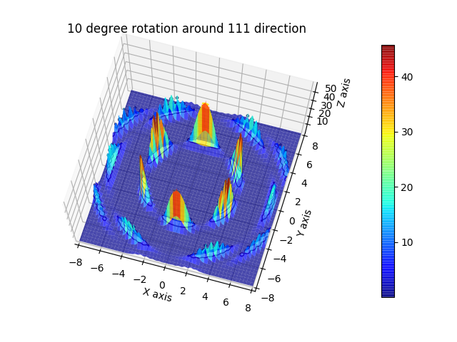
Ewald Sphere of simple cubic lattice
import jscatter as js
import numpy as np

import matplotlib.pyplot as pyplot
from matplotlib import cm

phi, theta = np.meshgrid(np.r_[0:np.pi:45j], np.r_[0:2 * np.pi:90j])

# The Cartesian coordinates of the sphere
q = 3
x = q * (np.sin(phi) * np.cos(theta) + 1)
y = q * np.sin(phi) * np.sin(theta)
z = q * np.cos(phi)
qxzy = np.asarray([x, y, z]).reshape(3, -1).T

sclattice = js.lattice.scLattice(2.1, 5)
ffe = js.ff.orientedCloudScattering(qxzy, sclattice.XYZ, mosaicity=[5,0,0], nCone=20, rms=0.02)

# log scale for colors
ffey = np.log(ffe.Y)
fmax, fmin = ffey.max(), ffey.min()
ffeY = (np.reshape(ffey, x.shape) - fmin) / (fmax - fmin)

# Set the aspect ratio to 1 so our sphere looks spherical
fig = pyplot.figure(figsize=pyplot.figaspect(1.))
ax = fig.add_subplot(111, projection='3d')
ax.plot_surface(x, y, z, rstride=1, cstride=1, facecolors=cm.seismic(ffeY))

# Turn off the axis planes
ax.set_axis_off()
pyplot.show(block=False)

# ------------------------------------

phi, theta = np.meshgrid(np.r_[0:np.pi:90j], np.r_[0:1 * np.pi:90j])
# The Cartesian coordinates of the unit sphere
q = 8
x = q * (np.sin(phi) * np.cos(theta) + 1)
y = q * np.sin(phi) * np.sin(theta)
z = q * np.cos(phi)
qxzy = np.asarray([x, y, z]).reshape(3, -1).T

# Set the aspect ratio to 1 so our sphere looks spherical
fig = pyplot.figure(figsize=pyplot.figaspect(1.))
ax = fig.add_subplot(111, projection='3d')

# create lattice and show it scaled
sclattice = js.lattice.scLattice(2.1, 1)
sclattice.rotatehkl2Vector([1, 1, 1], [0, 0, 1])
gg = ax.scatter(sclattice.X / 3 + q, sclattice.Y / 3, sclattice.Z / 3, c='k', alpha=0.9)
gg.set_visible(True)

ds = 15
fpi = np.pi / 180.
ffs = js.sf.orientedLatticeStructureFactor(qxzy, sclattice, rotation=None, domainsize=ds, rmsd=0.1, hklmax=2, nGauss=23)
# show scattering in log scale on Ewald sphere
ffsy = np.log(ffs.Y)
fmax, fmin = ffsy.max(), ffsy.min()
ffsY = (np.reshape(ffsy, x.shape) - fmin) / (fmax - fmin)

ax.plot_surface(x, y, z, rstride=1, cstride=1, facecolors=cm.hsv(ffsY), alpha=0.4)
ax.plot([q, 2 * q], [0, 0], [0, 0], color='k')
pyplot.show(block=False)

#  ad flat detector xy plane
xzw = np.mgrid[-8:8:80j, -8:8:80j]
qxzw = np.stack([np.zeros_like(xzw[0]), xzw[0], xzw[1]], axis=0)

ff2 = js.sf.orientedLatticeStructureFactor(qxzw.reshape(3, -1).T, sclattice, rotation=None, domainsize=ds, rmsd=0.1,
                                           hklmax=2, nGauss=23)
ffs2 = np.log(ff2.Y)
fmax, fmin = ffs2.max(), ffs2.min()
ff2Y = (np.reshape(ffs2, xzw[0].shape) - fmin) / (fmax - fmin)
ax.plot_surface(qxzw[0], qxzw[1], qxzw[2], rstride=1, cstride=1, facecolors=cm.gist_ncar(ff2Y), alpha=0.3)
ax.set_xlabel('x axis')
ax.set_ylabel('y axis')
ax.set_zlabel('z axis')

fig.suptitle('Scattering plane and Ewald sphere of lattice \nmatplotlib is limited in 3D')
pyplot.show(block=False)
# matplotlib is not real 3D rendering
# maybe use later something else
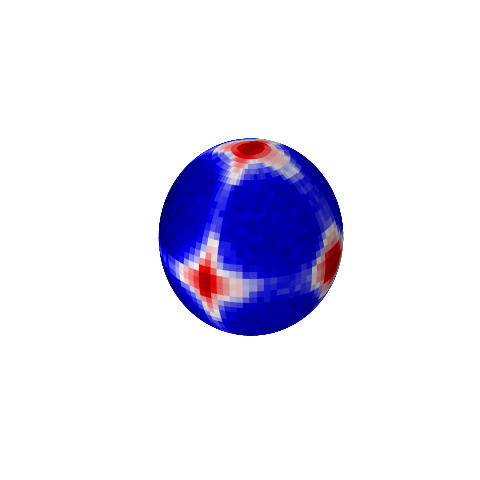
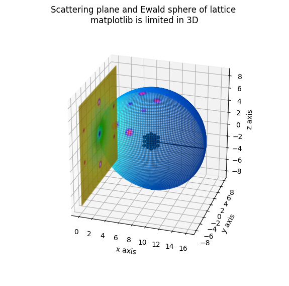
12.5.10. A nano cube build of different lattices
Here we build a nano cube from different crystal structures.
We can observe the cube formfactor and at larger Q the crystal peaks broadened by the small size. The scattering is explicitly calculated from the grids by ff.cloudScattering. Smoothing with a Gaussian considers experimental broadening (and smooth the result:-).
relError is set to higher value to speed it up. For precise calculation decrease it. For the pictures it was 0.02, this takes about 26 s on 6 core CPU for last bcc example with about 10000 atoms and 900 Q values.
Model with explicit atom positions in small grid
The peaks at large Q are Bragg peaks. Due to the small size extinction rules are not fulfilled completely, which is best visible at first peak positions where we still observe forbidden peaks for bcc and fcc. All Bragg peaks are shown in the second example. The formfactor shows reduced amplitudes due to Debye-Waller factor (rms) and the number of grid atoms. The analytical solution has infinite high density of atoms and a sharp interface.
import jscatter as js
import numpy as np

q = np.r_[js.loglist(0.01, 3, 200), 3:40:800j]
unitcelllength = 1.5
N = 8
rms = 0.05
relError = 20  # 0.02 for picture below

# make grids and calc scattering
scgrid = js.sf.scLattice(unitcelllength, N)
sc = js.ff.cloudScattering(q, scgrid.points, relError=relError, rms=rms)
bccgrid = js.sf.bccLattice(unitcelllength, N)
bcc = js.ff.cloudScattering(q, bccgrid.points, relError=relError, rms=rms)
fccgrid = js.sf.fccLattice(unitcelllength, N)
fcc = js.ff.cloudScattering(q, fccgrid.points, relError=relError, rms=rms)
#
# plot  data
p = js.grace(1.5, 1)
# smooth with Gaussian to include instrument resolution
p.plot(sc.X, js.formel.smooth(sc, 10, window='gaussian'), legend='sc')
p.plot(bcc.X, js.formel.smooth(bcc, 10, window='gaussian'), legend='bcc')
p.plot(fcc.X, js.formel.smooth(fcc, 10, window='gaussian'), legend='fcc')
#
# diffusive scattering
# while cloudScattering is normalized to one (without normalization ~ N**2),
# diffusive is proportional to scattering of single atoms (incoherent ~ N)
q = q = js.loglist(1, 35, 100)
p.plot(q, (1 - np.exp(-q * q * rms ** 2)) / scgrid.numberOfAtoms(), li=[3, 2, 1], sy=0, le='sc diffusive')
p.plot(q, (1 - np.exp(-q * q * rms ** 2)) / bccgrid.numberOfAtoms(), li=[3, 2, 2], sy=0, le='bcc diffusive')
p.plot(q, (1 - np.exp(-q * q * rms ** 2)) / fccgrid.numberOfAtoms(), li=[3, 2, 3], sy=0, le='fcc diffusive')
#
# cuboid formfactor for small Q
q = js.loglist(0.01, 2, 300)
cube = js.ff.cuboid(q, unitcelllength * (2 * N + 1))
p.plot(cube.X, js.formel.smooth(cube, 10, window='gaussian') / cube.Y[0], sy=0, li=1, le='cube form factor')
#
p.title('Comparison sc, bcc, fcc lattice for a nano cube')
p.yaxis(scale='l', label='I(Q)', max=1, min=5e-7)
p.xaxis(scale='l', label=r'Q / A\S-1', max=50, min=0.01)
p.legend(x=0.02, y=0.001, charsize=1.5)
p.text('cube formfactor', x=0.02, y=0.05, charsize=1.4)
p.text('Bragg peaks', x=4, y=0.05, charsize=1.4)
p.text('diffusive scattering', x=4, y=1e-6, charsize=1.4)
p.save('LatticeComparison.png')
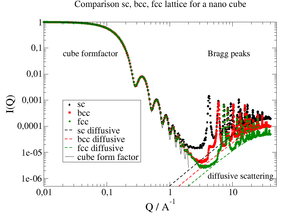
Analytical model assuming crystal lattice with limited size
This shows the Bragg peaks of crystal structures with broadening due to limited size.
The low Q scattering from the chrystal shape is not covered well as only the asymptotic behavior is governed.
import jscatter as js
import numpy as np

q = np.r_[js.loglist(0.5, 3, 50), 3:80:1200j]
unitcelllength = 1.5
N = 8
a = 1.5  # unit cell length
domainsize = a * (2 * N + 1)
rms = 0.05
p = js.grace(1.5, 1)
p.title('structure factor for sc, bcc and fcc 3D lattice')
p.subtitle('with diffusive scattering,asymmetry factor beta=1')

scgrid = js.sf.scLattice(unitcelllength, N)
sc = js.sf.latticeStructureFactor(q, lattice=scgrid, rmsd=rms, domainsize=domainsize)
p.plot(sc, li=[1, 3, 1], sy=0, le='sc')
p.plot(sc.X, 1 - sc[-3], li=[3, 2, 1], sy=0)  # diffusive scattering

bccgrid = js.sf.bccLattice(unitcelllength, N)
bcc = js.sf.latticeStructureFactor(q, lattice=bccgrid, rmsd=rms, domainsize=domainsize)
p.plot(bcc, li=[1, 3, 2], sy=0, le='bcc')
p.plot(bcc.X, 1 - bcc[-3], li=[3, 2, 2], sy=0)

fccgrid = js.sf.fccLattice(unitcelllength, N)
fcc = js.sf.latticeStructureFactor(q, lattice=fccgrid, rmsd=rms, domainsize=domainsize)
p.plot(fcc, li=[1, 3, 3], sy=0, le='fcc')
p.plot(fcc.X, 1 - fcc[-3], li=[3, 2, 3], sy=0)

p.text(r"broken lines \nshow diffusive scattering", x=10, y=0.1)
p.yaxis(label='S(q)', scale='l', max=50, min=0.05)
p.xaxis(label=r'q / A\S-1', scale='l', max=50, min=0.5)
p.legend(x=1, y=30, charsize=1.5)
p.save('LatticeComparison2.png')
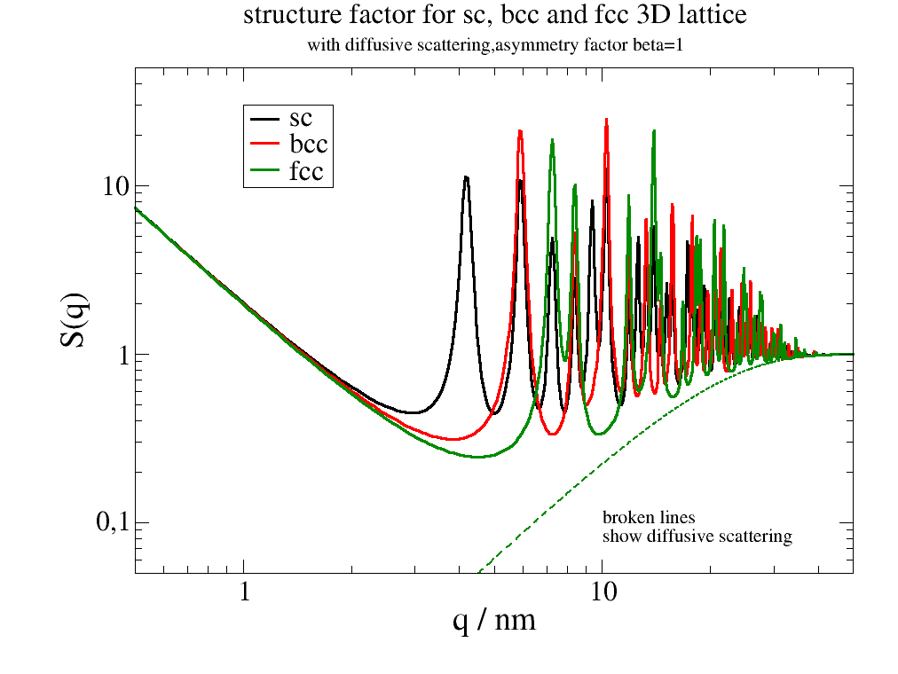
A direct comparison between both models for bcc cube
Differences are due to incomplete extinction of peaks and due to explicit dependence on the edges (incomplete elementary cells)
relError=0.02 samples until the error is smaller 0.02 for a q point with pseudorandom numbers. The same can be done with relError=400 on a fixed Fibonacci lattice. Both need longer for the computation.
The 1/q² power law at low q for the analytic model results from integration over infinite, d=3 dimensional q space. For a real nanoparticle or crystal domain the size (~ integration volume ) is finite resulting in the typical formfactor behavior with a plateau for lowest q, a Guinier range determined by Rg and a Porod region at higher q dependent on the fractal structure.
formfactor behavior with a plateau for lowest q, a Guinier range determined by Rg
and a Porod region at higher q dependent on the fractal structure.

#end3
"""

import jscatter as js
import numpy as np

q = np.r_[js.loglist(0.1, 3, 100), 3:40:800j]
unitcelllength = 1.5
N = 8
rms = 0.05
relError = 20  # 0.02 for the picture below
domainsize = unitcelllength * (2 * N + 1)

bccgrid = js.sf.bccLattice(unitcelllength, N)
bcc = js.ff.cloudScattering(q, bccgrid.points, relError=relError, rms=rms)
p = js.grace(1.5, 1)
p.plot(bcc.X, js.formel.smooth(bcc, 10, window='gaussian') * bccgrid.numberOfAtoms(), legend='bcc explicit')

q = np.r_[js.loglist(0.1, 3, 200), 3:40:1600j]
sc = js.sf.latticeStructureFactor(q, lattice=bccgrid, rmsd=rms, domainsize=domainsize)
p.plot(sc, li=[1, 3, 4], sy=0, le='bcc analytic')
p.yaxis(scale='l', label='I(Q)', max=20000, min=0.05)
p.xaxis(scale='l', label=r'Q / A\S-1', max=50, min=0.1)
p.legend(x=0.5, y=1000, charsize=1.5)
p.title('Comparison explicit and implicit model for a crystal cube')
p.text('cube formfactor', x=0.11, y=1, charsize=1.4)
p.text('bcc Bragg peaks', x=4, y=100, charsize=1.4)
p.text('diffusive scattering', x=10, y=0.1, charsize=1.4)
p.save('LatticeComparison3.png')
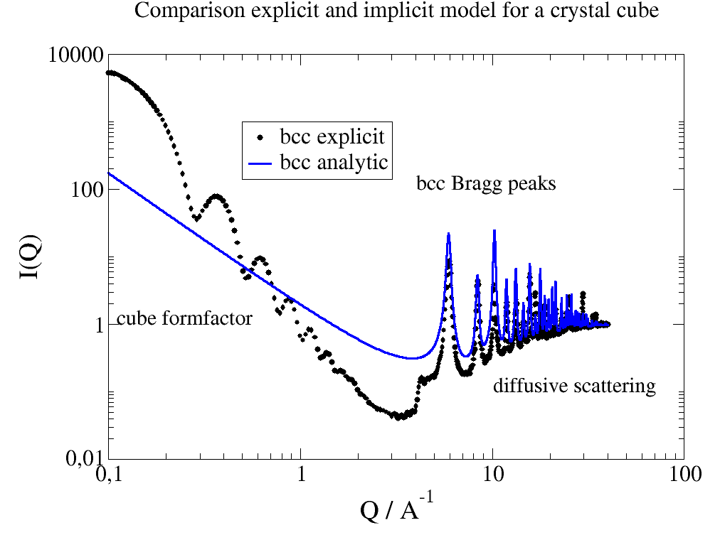
12.5.11. Linear Pearls with connecting coils
The example uses cloudscattering to build a line of spheres.
Between the spheres are Gaussian coils to represent chains connecting the spheres.
The model linearPearls() is very similar build
but uses a simpler build of the linear chain.
import jscatter as js
import numpy as np

q = js.loglist(0.01, 5, 300)

# create array containing formfactors
# columns will be [q, sphere, gaussian chain]
ffs = js.ff.sphere(q[::2], 3)
ffg = js.ff.gaussianChain(q[::2], 0.1)
ff = ffs.addColumn(1, ffg.Y)

# line of points
scl = js.sf.scLattice(8, [2, 0, 0])
# alternating sphere [1] anf gaussian coils [2]
grid1 = np.c_[scl.points, np.r_[[1] * 5]]
grid1[::2, -1] = 2

# grid points have default b=1
# we change gaussians to fa
p = js.grace()
for i, fa in enumerate([0.05, 0.1, 0.2, 0.5, 1], 1):
    grid1[::2, -2] = fa
    fq = js.ff.cloudScattering(q, grid1, relError=0, formfactoramp=ff)
    p.plot(fq, sy=[1, 0.4, i], le='gaussian coils fa={0:.2f}'.format(fa))

p.yaxis(scale='l', label='I(Q)')
p.xaxis(scale='l', label=r'Q / nm\S-1')
p.title('connected linear pearls')
p.subtitle('increasing mass in gaussians')
p.legend(x=0.02, y=0.1)
p.save('connected_linearPearls.png', size=(3, 3), dpi=150)

# same with orientation in 2D
grid1[::2, -2] = 0.1
qxzw = np.mgrid[-6:6:50j, -6:6:50j].reshape(2, -1).T
ffe = js.ff.orientedCloudScattering(qxzw, grid1, mosaicity=[5,0,0], nCone=10, rms=0)
fig = js.mpl.surface(ffe.X, ffe.Z, ffe.Y)
fig.axes[0].set_title(r'cos**2 for Z and slow decay for X due to 5 degree cone')
fig.show()
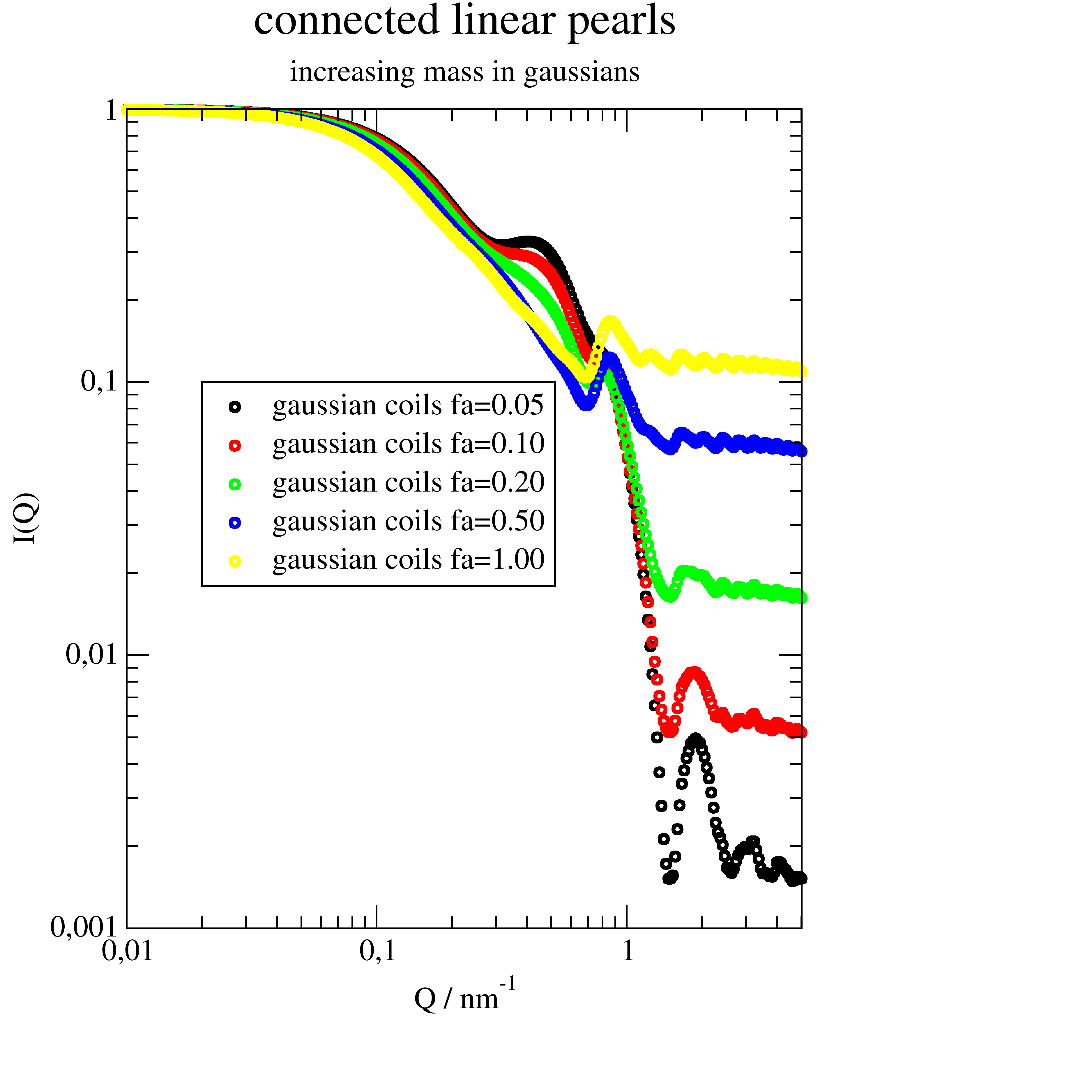
12.6. Dynamic models
This shows dynamic models and how to fit inelastic neutron scattering data from backscattering or time of flight experiments. The classical models are in the module dynamic and can be combined similar to the first example. The actual way how data are combined depends on the idea which atoms contribute to which process. This is more visible in later examples.
One example shows how to fit different instruments together.
Some dynamic models related to bio are shown in Biomacromolecules (bio).
12.6.1. Multi component models for data inspection at inelastic instruments
Here we use a simple two Lorentz model for data inspection or as general receip. The model can be adopted to the needs of the experiment mixing different models e.g translational diffusion and sidechains diffusion in a harmonic potential.
A more complex model that includes that all atoms contribute to COM diffusion and only a part to faster movements is shown later.
As resolution we use normalized experimental data to make it simple and stay close to the experiment.
As simple yet powerful predefined models doubleStretchedExp_w()
and threeLorentz_w() can be used in the same way.
Many published papers dont go beyond these simple models.
The data in the example were measured by Margarita Kruteva and Benedetta Rosi at EMU@ANSTO and the empty cell measurement is already subtracted in Mantid.
import jscatter as js
import numpy as np
from jscatter.dynamic import convolve
from jscatter.dynamic import lorentz_w

js.usempl(True)

def readinx(filename, block, l2p, instrument):
    # reusable function for inx reading
    # neutron scatterers use strange data formats like .inx dependent on instrument and local contact
    # blocks start with number of channels. Spaces around the number (' 562 ') are important to find the starting line.
    # this might dependent on instrument
    data = js.dL(filename,
                 block=block,  # this finds the starting of the blocks of all angles or Q
                 usecols=[1, 2, 3],  # ignore the numbering at each line
                 lines2parameter=l2p)  # catch the parameters at beginning
    for da in data:
        da.channels = da.line_1[0]
        da.Q = da.line_3[0]  # in 1/A  # it might be necessary to calc the Q here
        da.incident_energy = da.line_3[1]  # in meV
        da.temperature = da.line_3[3]  # in K if given
        da.instrument = instrument
    return data

# data exported from Mantid look different, simpler. These have only the parameter Q in front of a block
# these can be read like this e.g. from EMU exported by Mantid
def readEMUdat(filename, wavelength=6.27084, temperature=0):
    """
    Read data form EMU@ANSTO as direct output from Mantid (No .inx conversion needed)
    """
    data = js.dL(filename, delimiter=',')
    for da in data:
        da.Q = np.round(float(da.comment[0]), 4)
        da.temperature = temperature
        da.wavelength = wavelength
    # cut the zero at the end
    for i in range(len(data)):
        data[i] = data[i, :, :-1]
    return data

def lo2_fitmodel(w, dw, Q, amp1, amp2, fwhm1, fwhm2, elastic, bgr, resolution, wmax=None):
    """
    Model : elastic with two Lorentz functions and using experimental data for resolution convolution.

    w : frequencies 1/ns
    dw : center shift
    amp, amp2 : Lorentz amplitudes
    fwhw1,fwhw2 : full width half maximum pf Lorentz
    elastic : amplitude elastic contribution
    bgr : const background
    resolution : datalist with measured resolution and parameters Q same as in fit data
    wmax : cutoff frequency for resolution


    """
    if wmax is None:
        wmax = max(np.abs(w))

    # get right Q value of resolution for selected vana and prune to max frequency
    resolutionQ = resolution.filter(Q=Q)[0]

    # two Lorentz model and elastic , all same w
    model1 = lorentz_w(w, fwhm1)
    model1.Y = amp1 * model1.Y
    # model2 = transDiff_w(w, q=Q, D=Dt) # alternative model; parameters need to be adopted
    model2 = lorentz_w(w, fwhm2)
    model2.Y = amp1 * model2.Y

    # sum amplitudes and put in copied lorentz1
    both = model1.copy()
    both.Y = model1.Y + model2.Y

    # convolve with resolution; convolve also intermediate steps to use in later plots
    convboth = convolve(both, resolutionQ.prune(-wmax, wmax, weight=None), normB=True).interpolate(w)
    convmodel1 = convolve(model1, resolutionQ.prune(-wmax, wmax, weight=None), normB=True).interpolate(w)
    convmodel2 = convolve(model2, resolutionQ.prune(-wmax, wmax, weight=None), normB=True).interpolate(w)

    #  compose the data to return
    # use resolution as elastic contribution
    result = js.dA(np.c_[w,                                           # frequencies
                         convboth.Y + elastic * resolutionQ.Y + bgr,  # fit model
                         convmodel1.Y + bgr,                          # component 1
                         convmodel2.Y + bgr,                          # component 2
                         elastic*resolutionQ.Y+bgr].T)                # elastic contribution

    # append some of the intermediate contributions and add columnames to access components later
    result.columnname = 'w;both;m1;m2;el'
    result.elastic = elastic
    result.fwhm1 = fwhm1
    result.fwhm2 = fwhm2
    result.amp1 = amp1
    result.amp2 = amp2

    return result


# load experimental resolution and convert to 1/ns
# For emu the block is  '  314 ' with 2 spaces in front of the number and 1 after
# resolution experimental data
vanae = readEMUdat(js.examples.datapath + '/sample_5K_Q.dat.gz', temperature=5)
vana = js.dynamic.convert_e2w(vanae, 0, unit='meV')
# convert resolution to normalized data that elastic has meaning
for va in vana:
    va.Y = va.Y/np.trapezoid(va.Y,va.X)

# read new data and convert to 1/ns
same = readEMUdat(js.examples.datapath + '/sample_413K_Q.dat.gz',temperature=413)
sam = js.dynamic.convert_e2w(same, 293, unit='meV')

# ----------------------------------------------------
# fit single dataset and plot addition thing in the errplot
n = 1
# sam[n].makeErrPlot(yscale='log', title=str(sam[1].Q) + ' A\S-1')
sam[n].setlimit()  # removes limits
sam[n].setlimit(elastic=[0, 10000], bgr=[0.0, 2])
sam[n].setlimit(amp1=[0], amp2=[0])  # no negative amplitudes
sam[n].setlimit(fwhm1=[1, 30], fwhm2=[0, 10])  # no negative and some max fwhm
sam[n].fit(model=lo2_fitmodel,
           freepar={'elastic': 0.7, 'bgr': 0.1, 'amp1': 1, 'amp2': 3, 'fwhm1': 20, 'fwhm2': 8, },
           fixpar={'dw': [0], 'wmax': 10,'resolution':vana},
           mapNames={'w': 'X'},
           method='Nelder-Mead', max_nfev=20000)

sam[n].showlastErrPlot(title='Q='+str(sam[n].Q)+' 1/A', yscale='log')
sam[n].errPlot(sam[n].lastfit.X,sam[n].lastfit._m1,sy=0,li=[1,2,3],le='Lorentz 1')  # add
sam[n].errPlot(sam[n].lastfit.X,sam[n].lastfit._m2,sy=0,li=[1,2,4],le='Lorentz 2')
sam[n].errPlot(sam[n].lastfit.X,sam[n].lastfit._el,sy=0,li=[1,2,5],le='elastic')
sam[n].errplot.Yaxis(min=1e-4,max=1)
sam[n].errplot.Save('inelasticInstruments_simple_residuals.png', size=(10, 8), dpi=100)

# ----------------------------------------------
# Fit one after the other
for n in np.r_[0:len(sam)]:
    # sam[n].makeErrPlot(yscale='log', title=str(sam[1].Q) + ' A\S-1')
    sam[n].setlimit()  # removes limits
    sam[n].setlimit(el=[0, 10000], bgr=[0.0, 1])
    sam[n].setlimit(amp1=[0], amp2=[0])  # no negative amplitudes
    sam[n].setlimit(fwhm1=[0, 30], fwhm2=[0, 30])  # no negative and some max fwhm
    sam[n].fit(lo2_fitmodel,
               {'elastic': 1, 'bgr': 1e-5, 'amp1': 1, 'amp2': 3, 'fwhm1': 20, 'fwhm2': 8,  },
               {'dw': [0], 'wmax': 6,'resolution':vana},
               {'w': 'X'},
               method='Nelder-Mead', max_nfev=20000)
    # sam[n].killErrPlot()  # close it , or uncomment to have them open
# look at one single errplot
n = 2
sam[n].showlastErrPlot(title='Q='+str(sam[n].Q)+' 1/A', yscale='log')
sam[n].errPlot(sam[n].lastfit.X,sam[n].lastfit._m1,sy=0,li=[1,2,3],le='Lorentz 1')  # add
sam[n].errPlot(sam[n].lastfit.X,sam[n].lastfit._m2,sy=0,li=[1,2,4],le='Lorentz 2')
sam[n].errPlot(sam[n].lastfit.X,sam[n].lastfit._el,sy=0,li=[1,2,5],le='elastic')
sam[n].errplot.Yaxis(min=1e-5,max=0.2)

# make plot of fit parameters
p1 = js.mplot()
p1.Plot(sam.Q, sam.fwhm1, sam.fwhm1)
p1.Plot(sam.Q, sam.fwhm2, sam.fwhm2)
# if you want to calculate somthing use .array
# p1.Plot(sam.Q, sam.fwhm1.array*sam.Q.array)
p1.Xaxis(label='Q')
p1.Yaxis(label='fwhm', scale='norm', min=0, max=50)  # scale='log' or 'norm'
The residual fit with components of first example above The quality of fits depends strongly on your model and this is a simple one.
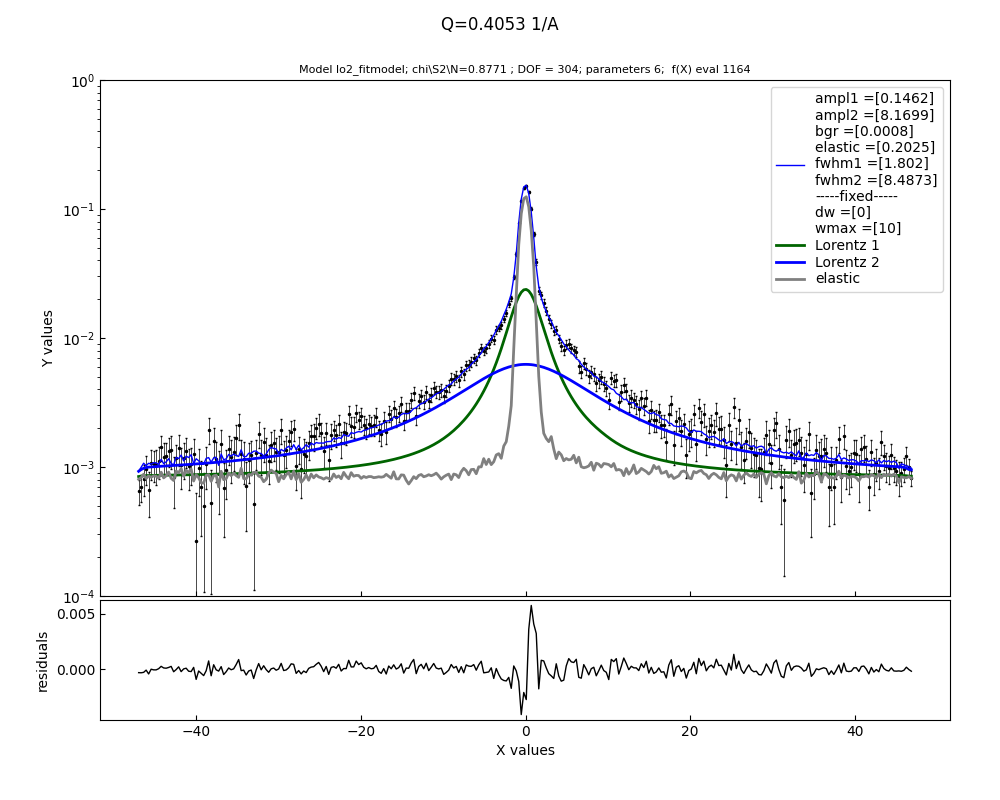
Continue with fit of all data together. Use ‘workers=0’ to speed up.
p1.Yaxis(label='fwhm', scale='norm', min=0, max=50)  # scale='log' or 'norm'


# -----------------------------------------------------
# fit all together , takes longer
# sam.makeErrPlot(yscale='log', title=str(sam.Q) + ' A\S-1')
sam.setlimit()  # removes limits
sam.setlimit(elastic=[0, 10000], bgr=[0.0, 2])
sam.setlimit(amp1=[0], amp2=[0])  # no negative amplitudes
sam.setlimit(fwhm1=[0, 30], fwhm2=[0, 30])  # no negative and some max fwhm

# here 'fwhm1': 0.0 means a common fit parameters and 'fwhm2': [0.001] is individual fit parameter
sam.fit(lo2_fitmodel,
        {'elastic': [1], 'bgr': [0.1], 'amp1': [1], 'amp2': [3], 'fwhm1': 20, 'fwhm2': [1], },
        {'dw': [0], 'wmax': 10,'resolution':vana},
        {'w': 'X'},
        method='lm', max_nfev=20000, workers=0)  # workers=1 uses only one cpu, =0 uses all
sam.showlastErrPlot(title='all together', yscale='log')

# ------------------------------------------------------
# inspect one of the overall fit
n = 5  # which one to plot
p = js.mplot()
p.Yaxis(scale='log')
p.Title(f'Q={sam[n].Q} ')
p.Plot(sam[n])
p.Plot(sam.lastfit[n], sy=0, li=[1, 2, 14], le='fit')
p.Plot(sam.lastfit[n].X, sam.lastfit[n]._m1, sy=0, li=[1, 2, 10], le='common fwhm1')
p.Plot(sam.lastfit[n].X, sam.lastfit[n]._m2, sy=0, li=[2, 2, 4], le='individual fwhm2')
p.Plot(sam.lastfit[n].X, sam.lastfit[n]._el, sy=0, li=[3, 2, 6], le='elastic')
p.Legend()
# p.Save('inelasticInstruments_simple.png', size=(5, 4), dpi=400)
Look at a dataset of the fit of all together.
The quality of fits depends strongly on your model and this is a simple one.
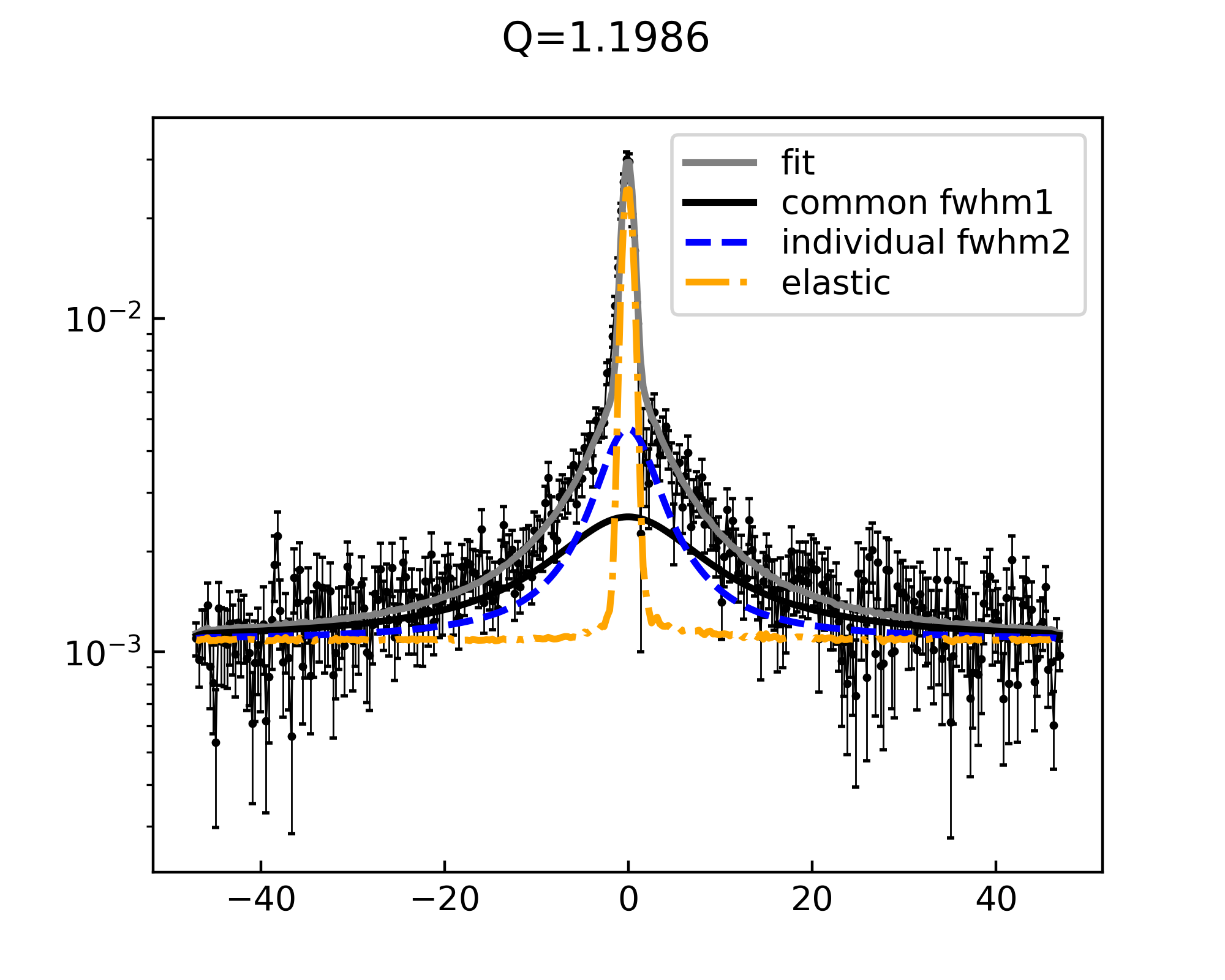
12.6.2. Fit multiple quasielastic instruments together
A model for incoherent scattering neglecting coherent and maybe some other contributions
We use real data (spheres@MLZ) but a strongly simplified model ignoring rotational diffusion of the protein, D2O contribution and dihedral CH3 motions visible in IN5 data. Therefore the results are yet not to over interpret even if the diffusion coefficient is not bad.
Also counts from background and empty cell might be present.
The intention is to give a relative simple example how to fit different instruments together taking into account the different resolutions and maybe time domain and frequency domain.
The combined fit allows common parameters as diffusion coefficient,fraction of localised motions with same rmsd and tau but still individual amplitudes and backgrounds.
# The intention is to give an example how to fit different instruments together

import jscatter as js
import numpy as np
from jscatter.dynamic import convolve
from jscatter.dynamic import diffusionHarmonicPotential_w, transDiff_w


def readinx(filename, block, l2p, instrument):
    # reusable function for inx reading
    # neutron scatterers use strange data formats like .inx dependent on local contact
    # the blocks start with  number of channels. Spaces (' 562 ') are important to find the starting line.
    # this might dependent on instrument
    data = js.dL(filename,
                 block=block,  # this finds the starting of the blocks of all angles or Q
                 usecols=[1, 2, 3],  # ignore the numbering at each line
                 lines2parameter=l2p)  # catch the parameters at beginning
    for da in data:
        da.channels = da.line_1[0]
        da.Q = da.line_3[0]  # in 1/A
        da.incident_energy = da.line_3[1]  # in meV
        da.temperature = da.line_3[3]  # in K if given
        da.instrument = instrument
    return data

# recover fit of resolution
# see js.dynamic.resolution_w in examples how this was fitted
vana_spheres = js.dL(js.examples.datapath + '/Vana_fitted.inx.gz')
vana_spheres.getfromcomment('modelname')

# read new data
adh = readinx(js.examples.datapath + '/ADH.inx.gz', block=' 563 ', l2p=[-1, -2, -3, -4, -5],instrument='spheres')

# convert to 1/ns
adhf = js.dynamic.convert_e2w(adh, 293, unit='μeV')


def trs_fitmodel(wt, dw, Q, DD, floc, tau, rmsd, A, bgr, instrument):
    """
    Assume NSE data (WASP@ILL) and backscattering (BS) data.
    BS need the convolution with resolution while NSE data are always resolution corrected.

    wt : times from NSE or frequencies from BS
    other input as above

    Here we assume that the resolution measurements are fitted by multiple Gaussians .
    Experimental data can also be used like in other examples
    """
    if instrument in ['spheres','in5']:
        w = wt  # increase w to avoid boundary effects
        # get right Q value of resolution for selected instrument
        if instrument == 'spheres':
            resolutionQ = vana_spheres.filter(Q=Q)[0]
            resolution = js.dynamic.resolution_w(w=w, resolution=resolutionQ)
        elif instrument == 'IN5':
            resolutionQ = vana_IN5.filter(Q=Q)[0]
            resolution = js.dynamic.resolution_w(w=w, resolution=resolutionQ)

        # The model is the same for these instruments

        # localized diffusion in rmsd with tau
        loc = diffusionHarmonicPotential_w(w, Q, tau, rmsd)
        loc.Y = js.dynamic.elastic_w(w).Y * (1 - floc) + floc * loc.Y  # add elastic fraction
        locw = convolve(loc, resolution, normB=True)

        # translational diffusion
        trans = transDiff_w(w, Q, DD)
        transw = convolve(trans, resolution, normB=True)

        transloc = convolve(trans, loc)
        transloc.floc = floc

        res = convolve(transloc, resolution, normB=True)
        # add amplitude and background
        res.Y = A * res.Y + bgr
        res.X = res.X + resolutionQ.w0 + dw

        # append some of the intermediate contributions
        res = res.addColumn(1,A*transw.Y*(1-floc)+bgr)
        res = res.addColumn(1, A * locw.Y * floc + bgr)
        res = res.addColumn(1,resolution.interp(wt)+bgr)
        res.columnname='w;tl;t;l;r'  # name the columns for easier access

    elif instrument == 'JNSE':
        # a NSE machine operating in time domain needs a different model (not yet)
        t = wt
        res = transrotsurf(t, Q, DD, floc, tau, rmsd)

    # interpolate to needed scale points
    return res.interpAll(wt)

# use reduce data for first faster fitting; use all later
adh2 = adhf[1::3]

# fit single dataArray
ad = adh2[-1]
ad.makeErrPlot(yscale='log', title=str(ad.Q) + ' A\S-1')
ad.setlimit(A=[0, 10000], bgr=[0, 10], DD=[0.005, 10], floc=[0.1, 0.9, 0, 1], tau=[0, 2], rmsd=[0, 20],dw=[-2,2])
ad.fit(trs_fitmodel,
       {'A': 90, 'DD': 0.5,'bgr': 1,  'floc': 0.8, 'tau': 0.1, 'rmsd': 1,'dw':0},
       {},
       {'wt': 'X'},
       method='Nelder-Mead',max_nfev=20000)

ad.errplot.plot(ad.lastfit.X,ad.lastfit._t,li=[1,3,2],sy=0,le='trans')
ad.errplot.plot(ad.lastfit.X,ad.lastfit._l,li=[1,3,4],sy=0,le='loc')
ad.errplot.legend()


# fit all together with common DD, floc, rmsd, tau and independent A and bgr
ad5 = adhf[1::3]
ad5.makeErrPlot(yscale='log', title=fr'{str(ad5.Q)} A\S-1',residual='rel')
ad5.setlimit(A=[0, 10000], bgr=[0, 10], DD=[0.005, 10], floc=[0.01, 0.9, 0, 1], tau=[0, 20], rmsd=[0, 20],dw=[-2,2])
ad5.fit(trs_fitmodel,
        {'A': [90], 'DD': 0.05,'bgr': [1],  'floc': 0.8, 'tau': 0.1, 'rmsd': 1,},
        {'dw':[0]},
        {'wt': 'X'},
        max_nfev=20000)

ad5.savelastErrPlot('inelasticInstruments_together.png', size=(2, 1.5), dpi=400)

# check diffusion
ad5.DD
ad5.DD_err

# inspect one of the overall fit
p = js.grace()
p.yaxis(scale='log')
p.title(f'Q={ad5[-1].Q} A\S-1')
p.plot(ad5[-1])
p.plot(ad5.lastfit[-1],sy=0,li=[1,2,14],le='fit')
p.plot(ad5.lastfit[-1].X,ad5.lastfit[-1]._l,sy=0,li=[1,2,10],le='local')
p.plot(ad5.lastfit[-1].X,ad5.lastfit[-1]._t,sy=0,li=[1,2,4],le='diffusion')
p.legend()
p.save('inelasticInstruments_one.png', size=(2, 1.5), dpi=400)
Look at the fit of all together.
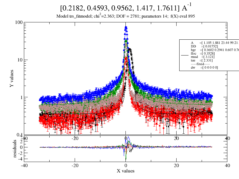
One Q value only
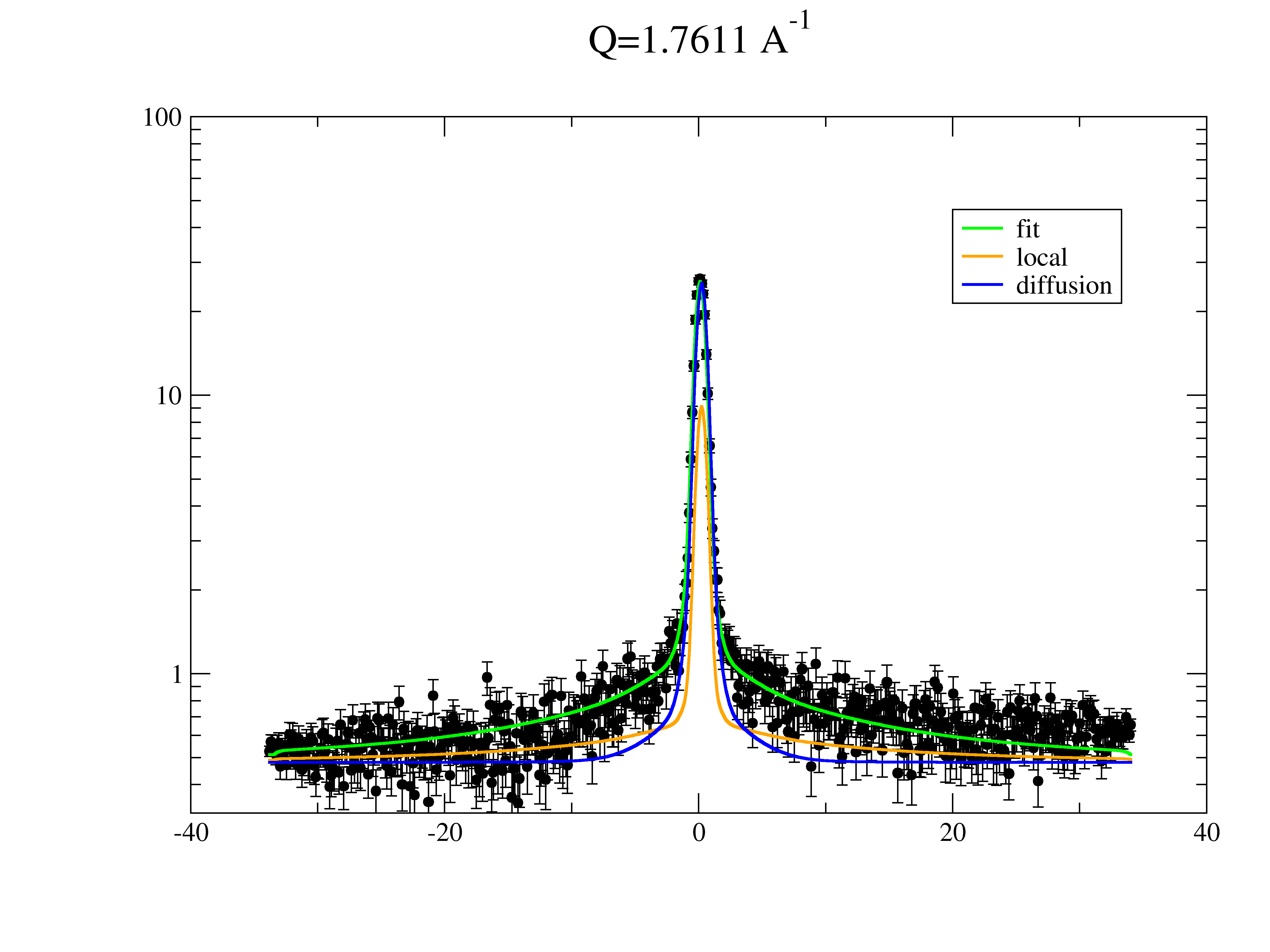
12.6.3. A comparison of different dynamic models in frequency domain
Compare different kinds of diffusion in restricted geometry by the HWHM from the spectra.
import jscatter as js
import numpy as np

# make a plot of the spectrum
w = np.r_[-100:100:1]
ql = np.r_[1:15:.5]
p = js.grace()
p.title('Inelastic neutron scattering ')
p.subtitle('diffusion in a sphere')
iqw = js.dL([js.dynamic.diffusionInSphere_w(w=w, q=q, D=0.14, R=0.2) for q in ql])
p.plot(iqw)
p.yaxis(scale='l', label='I(q,w) / a.u.', min=1e-6, max=1, )
p.xaxis(scale='n', label=r'w / ns\S-1', min=-100, max=100, )

# Parameters
ql = np.r_[0.5:15.:0.2]
D = 0.1
R = 0.5  # diffusion coefficient and radius
w = np.r_[-100:100:0.1]
u0 = R / 4.33 ** 0.5
t0 = R ** 2 / 4.33 / D  # corresponding values for Gaussian restriction, see Volino et al.

# In the following we calc the spectra and then extract the FWHM to plot it

# calc spectra
iqwD = js.dL([js.dynamic.transDiff_w(w=w, q=q, D=D) for q in ql[5:]])
iqwDD = js.dL([js.dynamic.time2frequencyFF(js.dynamic.simpleDiffusion, 'elastic', w=w, q=q, D=D) for q in ql])
iqwS = js.dL([js.dynamic.diffusionInSphere_w(w=w, q=q, D=D, R=R) for q in ql])
iqwG3 = js.dL([js.dynamic.diffusionHarmonicPotential_w(w=w, q=q, rmsd=u0, tau=t0, ndim=3) for q in ql])
iqwG2 = js.dL([js.dynamic.diffusionHarmonicPotential_w(w=w, q=q, rmsd=u0, tau=t0, ndim=2) for q in ql])
iqwG11 = js.dL([js.dynamic.t2fFF(js.dynamic.diffusionHarmonicPotential, 'elastic', w=w, q=q, rmsd=u0,
                                 tau=t0, ndim=1) for q in ql])
iqwG22 = js.dL([js.dynamic.t2fFF(js.dynamic.diffusionHarmonicPotential, 'elastic', w=w, q=q, rmsd=u0,
                                 tau=t0, ndim=2) for q in ql])
iqwG33 = js.dL([js.dynamic.t2fFF(js.dynamic.diffusionHarmonicPotential, 'elastic', w=w, q=q, rmsd=u0,
                                 tau=t0, ndim=3) for q in ql])
# iqwCH3=js.dL([js.dynamic.t2fFF(js.dynamic.methylRotation,'elastic',w=w,q=q ) for q in ql])

# plot HWHM  in a scaled plot
p1 = js.grace(1.5, 1.5)
p1.title('Inelastic neutron scattering models')
p1.subtitle('Comparison of HWHM for different types of diffusion')
p1.plot([0.1, 60], [4.33296] * 2, li=[1, 1, 1], sy=0)
p1.plot((R * iqwD.wavevector.array) ** 2, [js.dynamic.getHWHM(dat)[0] / (D / R ** 2) for dat in iqwD], sy=[1, 0.5, 1],
        le='free')
p1.plot((R * iqwS.wavevector.array) ** 2, [js.dynamic.getHWHM(dat)[0] / (D / R ** 2) for dat in iqwS], sy=[2, 0.5, 3],
        le='in sphere')
p1.plot((R * iqwG3.wavevector.array) ** 2, [js.dynamic.getHWHM(dat)[0] / (D / R ** 2) for dat in iqwG3], sy=[3, 0.5, 4],
        le='harmonic 3D')
p1.plot((R * iqwG2.wavevector.array) ** 2, [js.dynamic.getHWHM(dat)[0] / (D / R ** 2) for dat in iqwG2], sy=[4, 0.5, 7],
        le='harmonic 2D')
p1.plot((R * iqwDD.wavevector.array) ** 2, [js.dynamic.getHWHM(dat)[0] / (D / R ** 2) for dat in iqwDD], sy=0,
        li=[1, 2, 7], le='free fft')
p1.plot((R * iqwG11.wavevector.array) ** 2, [js.dynamic.getHWHM(dat, gap=0.04)[0] / (D / R ** 2) for dat in iqwG11],
        sy=0, li=[1, 2, 1], le='harmonic 1D fft')
p1.plot((R * iqwG22.wavevector.array) ** 2, [js.dynamic.getHWHM(dat, gap=0.04)[0] / (D / R ** 2) for dat in iqwG22],
        sy=0, li=[2, 2, 1], le='harmonic 2D fft')
p1.plot((R * iqwG33.wavevector.array) ** 2, [js.dynamic.getHWHM(dat, gap=0.04)[0] / (D / R ** 2) for dat in iqwG33],
        sy=0, li=[3, 2, 1], le='harmonic 3D fft')
# 1DGauss as given in the reference (see help for this function) seems to have a mistake
# Use the t2fFF from time domain
# p1.plot((0.12*iqwCH3.wavevector.array)**2,[js.dynamic.getHWHM(dat,gap=0.04)[0]/(D/0.12**2) for dat in iqwCH3],
#                                                                             sy=0,li=[1,2,4], le='1D harmonic')


# jump diffusion
r0 = .5
t0 = r0 ** 2 / 2 / D
w = np.r_[-100:100:0.02]
iqwJ = js.dL([js.dynamic.jumpDiff_w(w=w, q=q, r0=r0, t0=t0) for q in ql])
ii = 54
p1.plot((r0 * iqwJ.wavevector.array[:ii]) ** 2, [js.dynamic.getHWHM(dat)[0] / (D / r0 ** 2) for dat in iqwJ[:ii]])
p1.text(r'jump diffusion', x=8, y=1.4, rot=0, charsize=1.25)
p1.plot((R * iqwG33.wavevector.array) ** 2, (R * iqwG33.wavevector.array) ** 2, sy=0, li=[3, 2, 1])
p1.yaxis(min=0.3, max=100, scale='l', label='HWHM/(D/R**2)')
p1.xaxis(min=0.3, max=140, scale='l', label=r'(q*R)\S2')
p1.legend(x=0.35, y=80, charsize=1.25)
# The finite Q resolution results in  js.dynamic.getHWHM (linear interpolation to find [max/2])
# in an offset for very narrow spectra
p1.text(r'free diffusion', x=8, y=10, rot=45, color=2, charsize=1.25)
p1.text(r'free ', x=70, y=65, rot=0, color=1, charsize=1.25)
p1.text(r'3D ', x=70, y=45, rot=0, color=4, charsize=1.25)
p1.text(r'sphere', x=70, y=35, rot=0, color=3, charsize=1.25)
p1.text(r'2D ', x=70, y=15, rot=0, color=7, charsize=1.25)
p1.text(r'1D ', x=70, y=7, rot=0, color=2, charsize=1.25)
p1.save('DynamicModels.png', size=(3, 3), dpi=150)
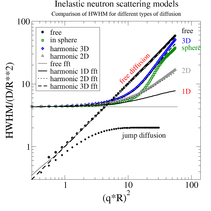
12.6.4. Protein incoherent scattering in frequency domain
We look at a protein in solution that shows translational and rotational diffusion with atoms local restricted in a harmonic potential.
This is what is expected for the incoherent scattering of a protein (e.g. at 50mg/ml concentration). The contribution of methyl rotation is missing.
- For details see :
Fast internal dynamics in alcohol dehydrogenase, The Journal of Chemical Physics 143, 075101 (2015), https://doi.org/10.1063/1.4928512
Here we use a reading of a PDB structure with only CA atoms for a simple model. This can be improved using the bio module accessing positions and selecting hydrogen atoms or adding coherent scattering.
First we look at the separate contributions :
# A model for protein incoherent scattering
# neglecting coherent and maybe some other contributions

import jscatter as js
import numpy as np
import urllib
from jscatter.dynamic import convolve as conv
from jscatter.dynamic import transDiff_w
from jscatter.dynamic import rotDiffusion_w
from jscatter.dynamic import diffusionHarmonicPotential_w

# get pdb structure file with 3rn3 atom coordinates and filter for CA positions in A
# this results in C-alpha representation of protein Ribonuclease A.
url = 'https://files.rcsb.org/download/3RN3.pdb'
pdbtxt = urllib.request.urlopen(url).read().decode('utf8')
CA = [line[31:55].split() for line in pdbtxt.split('\n') if line[13:16].rstrip() == 'CA' and line[:4] == 'ATOM']
# conversion to nm and center of mass
ca = np.array(CA, float) / 10.
cloud = ca - ca.mean(axis=0)
Dtrans = 0.086  # nm**2/ns  for 3rn3 in D2O at 20°C
Drot = 0.0163  # 1/ns
natoms = cloud.shape[0]

# A list of wavevectors and frequencies and a resolution.
# If bgr is zero we have to add it later after the convolution with resolution as constant instrument background.
# As resolution a single q independent (unrealistic) Gaussian is used.
ql = np.r_[0.1, 0.5, 1, 2:15.:2, 20, 30, 40]
w = np.r_[-100:100:0.1]
start = {'s0': 0.5, 'm0': 0, 'a0': 1, 'bgr': 0.00}
resolution = lambda w: js.dynamic.resolution_w(w=w, **start)
res = resolution(w)

# translational diffusion
p = js.grace(3, 0.75)
p.multi(1, 4)
p[0].title(' ' * 50 + 'Inelastic neutron scattering for protein Ribonuclease A', size=2)

iqwRtr = js.dL([conv(transDiff_w(w, q=q, D=Dtrans), res, normB=True) for q in ql])
iqwRt = js.dL([transDiff_w(w, q=q, D=Dtrans) for q in ql])

p[0].plot(iqwRtr, le='$wavevector')
p[0].plot(iqwRt, li=1, sy=0)
p[0].yaxis(min=1e-8, max=1e3, scale='l', ticklabel=['power', 0, 1], label=[r'I(Q,\xw\f{})', 1.5])
p[0].xaxis(min=-149, max=99, label=r'\xw\f{} / 1/ns', charsize=1)
p[0].legend(charsize=1, x=-140, y=1)
p[0].text(r'translational diffusion, one atom', y=80, x=-130, charsize=1.5)
p[0].text(r'Q / nm\S-1', y=2, x=-140, charsize=1.5)

# rotational diffusion
iqwRr = js.dL([rotDiffusion_w(w, q=q, cloud=cloud, Dr=Drot) for q in ql])
iqwRrr = js.dL([conv(iqw, res, normB=True) for iqw in iqwRr])

p[1].plot(iqwRr, li=1, sy=0)
p[1].plot(iqwRrr, le='$wavevector')
p[1].yaxis(min=1e-8, max=1e3, scale='l', ticklabel=['power', 0, 1, 'normal'])
p[1].xaxis(min=-149, max=99, label=r'\xw\f{} / 1/ns', charsize=1)
# p[1].legend()
p[1].text(r'rotational diffusion full cloud', y=50, x=-130, charsize=1.5)

# restricted diffusion in a harmonic local potential
# rmsd defines the size of the harmonic potential
iqwRgr = js.dL([conv(diffusionHarmonicPotential_w(w, q=q, tau=0.15, rmsd=0.3), res, normB=True) for q in ql])
iqwRg = js.dL([diffusionHarmonicPotential_w(w, q=q, tau=0.15, rmsd=0.3) for q in ql])

p[2].plot(iqwRgr, le='$wavevector')
p[2].plot(iqwRg, li=1, sy=0)
p[2].yaxis(min=1e-8, max=1e3, scale='l', ticklabel=['power', 0, 1], label='')
p[2].xaxis(min=-149, max=99, label=r'\xw\f{} / 1/ns', charsize=1)
# p[2].legend()
p[2].text(r'restricted diffusion one atom \n(harmonic)', y=50, x=-130, charsize=1.5)

# amplitudes at w=0 and w=10
p[3].title('amplitudes w=[0, 10]')
p[3].subtitle(r'\xw\f{}>10 restricted diffusion > translational diffusion')
ww = 10
wi = np.abs(w - ww).argmin()
p[3].plot(iqwRtr.wavevector, iqwRtr.Y.array.max(axis=1) * natoms, sy=[1, 0.3, 1], li=[1, 2, 1], le='trans + res')
p[3].plot(iqwRt.wavevector, iqwRt.Y.array.max(axis=1)* natoms, sy=[1, 0.3, 1], li=[2, 2, 1], le='trans ')
p[3].plot(iqwRt.wavevector, iqwRt.Y.array[:, wi]* natoms, sy=[2, 0.3, 1], li=[3, 3, 1], le='trans w=%.2g' % ww)
p[3].plot(iqwRrr.wavevector, iqwRrr.Y.array.max(axis=1), sy=[1, 0.3, 2], li=[1, 2, 2], le='rot + res')
p[3].plot(iqwRr.wavevector, iqwRr.Y.array.max(axis=1), sy=[1, 0.3, 2], li=[2, 2, 2], le='rot')
p[3].plot(iqwRr.wavevector, iqwRr.Y.array[:, wi], sy=[2, 0.3, 2], li=[3, 3, 2], le='rot w=%.2g' % ww)
p[3].plot(iqwRgr.wavevector, iqwRgr.Y.array.max(axis=1)* natoms, sy=[1, 0.3, 3], li=[1, 2, 3], le='restricted + res')
p[3].plot(iqwRg.wavevector, iqwRg.Y.array.max(axis=1)* natoms, sy=[8, 0.3, 3], li=[2, 2, 3], le='restricted')
p[3].plot(iqwRg.wavevector, iqwRg.Y.array[:, wi]* natoms, sy=[3, 0.3, 3], li=[3, 3, 3], le='restricted w=%.2g' % ww)

p[3].yaxis(min=1e-4, max=5e4, scale='l', ticklabel=['power', 0, 1, 'opposite'],
           label=[r'I(Q,\xw\f{}=[0,10])', 1, 'opposite'])
p[3].xaxis(min=0.1, max=50, scale='l', label=r'Q / nm\S-1', charsize=1)
p[3].legend(charsize=0.9, x=2.8, y=0.057)

p[3].text(r'translation', y=8e-1, x=15, rot=331, charsize=1.3, color=1)
p[3].text(r'rotation', y=6e1, x=15, rot=331, charsize=1.3, color=2)
p[3].text(r'harmonic', y=1e-1, x=15, rot=331, charsize=1.3, color=3)
p[3].text(r'\xw\f{}=10', y=1e-2, x=0.2, rot=30, charsize=1.5, color=1)
p[3].line(0.17, 5e-2, 0.17, 8e-3, 5, arrow=2, color=1)

p[3].text(r'resolution', y=2212, x=0.5, rot=0, charsize=1.5, color=4)

p[3].line(0.5, 100, 0.5, 25, 5, arrow=2, color=4)
p[3].line(0.5, 1500, 0.5, 300, 5, arrow=2, color=4)

p.save('inelasticNeutronScattering.png', size=(6, 1.5), dpi=400)
Blue arrows indicate the effect of instrument resolution at low Q. While rotation is always dominating, at \(\omega=10\) restricted diffusion (harmonic) is stronger than translational diffusion in midrange Q.
Now we add the above components to a combined model.
exR defines a radius from the center of mass that discriminates between fixed hydrogen inside
and hydrogen with additional restricted diffusion outside (close to the protein surface).
start = {'s0': 0.5, 'm0': 0, 'a0': 1, 'bgr': 0.00}
resolution = lambda w: js.dynamic.resolution_w(w=w, **start)


def transrotsurfModel(w, q, Dt, Dr, exR, tau, rmsd):
    """
    A model for trans/rot diffusion with a partial local restricted diffusion at the protein surface.

    See Fast internal dynamics in alcohol dehydrogenase The Journal of Chemical Physics 143, 075101 (2015);
    https://doi.org/10.1063/1.4928512

    Parameters
    ----------
    w   frequencies
    q   wavevector
    Dt  translational diffusion
    Dr  rotational diffusion
    exR outside this radius additional restricted diffusion with t0 u0
    tau  correlation time
    rmsd  Root mean square displacement Ds=u0**2/t0

    Returns
    -------

    """
    natoms = cloud.shape[0]
    trans = transDiff_w(w, q, Dt)
    trans.Y = trans.Y * natoms  # natoms contribute
    rot = rotDiffusion_w(w, q, cloud, Dr)  # already includes natoms
    fsurf = ((cloud ** 2).sum(axis=1) ** 0.5 > exR).sum()  # fraction of natoms close to surface
    loc = diffusionHarmonicPotential_w(w, q, tau, rmsd)
    # only fsurf atoms at surface contributes to local restricted diffusion, others elastic
    loc.Y = js.dynamic.elastic_w(w).Y * (natoms - fsurf) + fsurf * loc.Y

    final = conv(trans, rot)
    final = conv(final, loc)
    final.setattr(rot, 'rot_')
    final.setattr(loc, 'loc_')

    res = resolution(w)
    finalres = conv(final, res, normB=True)

    # finalres.Y+=0.0073  # background ?
    finalres.q = q
    finalres.fsurf = fsurf
    return finalres


ql = np.r_[0.1, 0.5, 1, 2, 4, 6, 10, 20]
p = js.grace(1, 1)
p.title('Protein incoherent scattering')
p.subtitle('Ribonuclease A')
iqwR = js.dL([transrotsurfModel(w, q=q, Dt=Dtrans, Dr=Drot, exR=0, tau=0.15, rmsd=0.3) for q in ql])
p.plot(iqwR[0], sy=0, li=[1, 2, 1], le='exR=0')
p.plot(iqwR[1:], sy=0, li=[1, 2, 1])
iqwR = js.dL([transrotsurfModel(w, q=q, Dt=Dtrans, Dr=Drot, exR=1, tau=0.15, rmsd=0.3) for q in ql])
p.plot(iqwR[0], sy=0, li=[1, 2, 2], le='exR=1')
p.plot(iqwR[1:], sy=0, li=[1, 2, 2])
iqwR = js.dL([transrotsurfModel(w, q=q, Dt=Dtrans, Dr=Drot, exR=1.4, tau=0.15, rmsd=0.3) for q in ql])
p.plot(iqwR[0], sy=0, li=[3, 3, 3], le='exR=1.4')
p.plot(iqwR[1:], sy=0, li=[3, 3, 3])
p.yaxis(min=1e0, max=2e5, label=r'I(q,\xw\f{})', scale='l', ticklabel=['power', 0, 1])
p.xaxis(min=0.1, max=100, label=r'\xw\f{} / ns\S-1', scale='l')
p.legend(x=0.2, y=1e1)

p[0].line(1, 5e2, 1, 5e1, 2, arrow=1)
p.text('resolution', x=0.9, y=7e1, rot=90)
p.text(r'q=2 nm\S-1', x=0.2, y=1e5, rot=0)
p.text(r'q=20 nm\S-1', x=0.2, y=8e2, rot=0)
p.text(r'q=3 nm\S-1', x=2, y=5e4, rot=0)
p.text(r'q=0.1 nm\S-1', x=2.2, y=1.5e2, rot=0)

p[0].line(0.17, 9e4, 0.17, 1e3, 2, arrow=2)
p[0].line(2, 1.5e2, 2, 4e4, 2, arrow=2)
p.text(r'Variation \nfixed/harmonic protons', x=1.2, y=4.44, rot=0)
p[0].line(7, 5.3, 12, 55, arrow=2)

p.save('Ribonuclease_inelasticNeutronScattering.png', size=(4, 4), dpi=150)
We observe that the elastic intensity first increases with Q and decreases again for \(Q>2 nm^{-1}\).
Variation of the fraction of hydrogen that show restricted diffusion is observable for midrange Q.
12.6.5. Hydrodynamic function
import numpy as np
import jscatter as js

# Hydrodynamic function and structure factor of hard spheres
# The hydrodynamic function describes how diffusion of spheres in concentrated suspension
# is changed due to hydrodynamic interactions.
# The diffusion is changed according to D(Q)=D0*H(Q)/S(Q)
# with the hydrodynamic function H(Q), structure factor S(Q)
# and Einstein diffusion of sphere D0

# some  wavevectors
q = np.r_[0:5:0.03]

p = js.grace(2, 1.5)
p.multi(1, 2)
p[0].title('Hydrodynamic function H(Q)')
p[0].subtitle('concentration dependence')
Rh = 2.2
for ii, mol in enumerate(np.r_[0.1:20:5]):
    H = js.sf.hydrodynamicFunct(q, Rh, molarity=0.001 * mol, )
    p[0].plot(H, sy=[1, 0.3, ii + 1], legend='H(Q) c=%.2g mM' % mol)
    p[0].plot(H.X, H[3], sy=0, li=[1, 2, ii + 1], legend='structure factor')

p[0].legend(x=2, y=2.4)
p[0].yaxis(min=0., max=2.5, label='S(Q); H(Q)')
p[0].xaxis(min=0., max=5., label=r'Q / nm\S-1')

# hydrodynamic function and structure factor of charged spheres
p[1].title('Hydrodynamic function H(Q)')
p[1].subtitle('screening length dependence')
for ii, scl in enumerate(np.r_[0.1:30:6]):
    H = js.sf.hydrodynamicFunct(q, Rh, molarity=0.0005, structureFactor=js.sf.RMSA,
                                structureFactorArgs={'R': Rh * 2, 'scl': scl, 'gamma': 5}, )
    p[1].plot(H, sy=[1, 0.3, ii + 1], legend='H(Q) scl=%.2g nm' % scl)
    p[1].plot(H.X, H[3], sy=0, li=[1, 2, ii + 1], legend='structure factor')

p[1].legend(x=2, y=2.4)
p[1].yaxis(min=0., max=2.5, label='S(Q); H(Q)')
p[1].xaxis(min=0., max=5., label=r'Q / nm\S-1')

p[0].text(r'high Q shows \nreduction in D\sself', x=3, y=0.22)
p[1].text(r'low Q shows reduction \ndue to stronger interaction', x=0.5, y=0.25)

p.save('HydrodynamicFunction.png')
12.6.6. Zimm dynamics including collective effects (H(Q)/S(Q)) on center of mass diffusion
A minimal example how to fit Iqt from NSE measurements on polyelectrolytes using finiteZimm to demonstrate how to include H(Q) and S(Q) for center of mass diffusion Dcm.
For details on the physics see
Interchain Hydrodynamic Interaction and Internal Friction of Polyelectrolytes Buvalaia, et al ACS Macro Letters 12(9):1218 https://doi.org/10.1021/acsmacrolett.3c00409
import jscatter as js
import numpy as np

# the structure factor type and parameters should be determined by fitting of SAXS/SANS data
# only for simplicity we use the PercusYevick, molarity is determined by experimental conditions of NSE
# here the experimental R of the PercusYevick is determined from experimental data

q0 = np.r_[0.01:2:100j]


def collectivefiniteZIMM(t, q, Dt=None, mu=0.5, Rh=4, R=4,tint=0, mol=0.0003):
    # Hq can be determined integrating over Sq and using Rh as a fit parameter
    # We assume here a polymer with different hydrodynamic interaction compared to a sphere
    # internally SF is calculated and saved in _sf
    SF = js.sf.PercusYevick
    HqSq = js.sf.hydrodynamicFunct(q0, Rh=Rh, molarity=mol,
                                 structureFactor=SF,
                                 structureFactorArgs={'R': R}, )
    HqSq.Y =  HqSq.Y / HqSq._sf  # this makes the needed H(Q)/S(Q)
    hqsq = HqSq[:2]  # only first columns

    # Dt is determined inside finiteZimm , but can be changed
    Iqt = js.dynamic.finiteZimm(t, q, NN=212, pmax=25, l=0.24, Dcm=Dt, tintern=tint, Temp=273 + 60, mu=mu,
                                viscosity=1, Dcmfkt = hqsq)
    Iqt.setColumnIndex(iey=None)
    return Iqt


# simulate data, typical NSE times IN15@ILL
tlist = js.loglist(0.1,300,30)

p = js.grace(2,1)
p.multi(1,2)
p[0].xaxis(label='t / ns',scale='log')
p[1].xaxis(label='t / ns',scale='log')
p[0].yaxis(label='I(Q,t)/I(Q,0)')

# lowest Q corresponds to DLS as synthetic dataset added to Iqt from NSE
sim = js.dL()
for q in np.r_[0.026,0.25,0.4,0.8,1.2,1.4,1.8]:  # in 1/nm
    sim.append(collectivefiniteZIMM(t=tlist, q=q, mol=0.0003, R=8, Rh=4, mu=0.6))
p[0].plot(sim,sy=0,li=[1,3,1])
p[1].plot(sim,sy=0,li=[1,3,1])

sim2 = js.dL()
for q in np.r_[0.026,0.25,0.4,0.6,0.8,1.2,1.4]:  # in 1/nm
    sim2.append(collectivefiniteZIMM(t=tlist, q=q, mol=0.0003, R=7, Rh=4, mu=0.6))
p[0].plot(sim2,sy=0,li=[3,3,2])

sim3 = js.dL()
for q in np.r_[0.026,0.25,0.4,0.6,0.8,1.2,1.4]:  # in 1/nm
    sim3.append(collectivefiniteZIMM(t=tlist, q=q, mol=0.0003, R=8, Rh=6, mu=0.6))
p[1].plot(sim3,sy=0,li=[3,3,4])

p[0].text('DLS',x=300,y=0.8)
p[1].text('DLS',x=300,y=0.8)
p[0].title('Interaction influences low Q, specifically DLS')
p[1].title('Rh influences all Q as self diffusion changes')

# p.save('collectiveZimm.png', size=(2, 1), dpi=150)

if 0:
    # A fit to exp. NSE data might be done like this (using sim as measured data, no errors)
    # fixpar are determined from other experiments
    sim.fit(model=collectivefiniteZIMM,
                freepar={'Rh':4,'mu':0.6,'tint':1},
                fixpar={'R':6, 'mol':0.0003 },  # from exp. conditions
                mapNames={'t':'X'})
Checkout the structure factor and HqSq to examine the Q dependent changes in the center of mass diffusion.
12.7. Biomacromolecules (bio)
Examples using the biomacromolecule module (bio) for protein and DNA scattering.
12.7.1. Load PDB structure and calc scattering
Load pdb protein structure from the PDB data bank by ID to scatteringUniverse. The pdb file is corrected and hydrogen is added automatically. The protein structure including H is saved to 3rn3_h.pdb.
import jscatter as js
import numpy as np

uni = js.bio.scatteringUniverse('3rn3')
uni.view()
uni.setSolvent('1d2o1')
uni.qlist = js.loglist(0.1, 5, 100)
# calc scattering both here in D2O
S = js.bio.nscatIntUniv(uni.select_atoms('protein'))
S = js.bio.xscatIntUniv(uni.select_atoms('protein'))

p = js.grace()
p.title('N scattering solvent matching')
p.yaxis(scale='l', label=r'I(Q) / nm\S2\N/particle')
p.xaxis(scale='l', label='Q / nm\S-1')

for x in np.r_[0:0.5:0.1]:
    uni.setSolvent([f'{x:.2f}d2o1',f'{1-x:.2f}h2o1' ])
    Sn = js.bio.nscatIntUniv(uni.select_atoms('protein'))
    p.plot(Sn, le=f'{x:.2f} D2O')

p.legend()
# p.save(js.examples.imagepath+'/biosolventmatching.jpg', size=(2, 2))
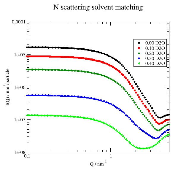
12.7.2. Protein scattering and effective diffusion
Protein scattering for different molecular weight proteins at 10 g/l concentration.
We assume here rigid protein structures without internal fluctuations. The diffusion corresponds accordingly to the rigid body diffusion of a protein.
See Exploring internal protein dynamics by neutron spin echo spectroscopy for details.
import jscatter as js
import numpy as np
import scipy.constants as constants

adh = js.bio.fetch_pdb('4w6z.pdb1')
# the 2 dimers in are in model 1 and 2 and need to be merged into one.
adhmerged = js.bio.mergePDBModel(adh)

p = js.grace(1.4, 1)
p.multi(1, 2)

for cc, pdb in enumerate(['3rn3', '3pgk', adhmerged], 1):
    # create universe; M and Z are for wrong named Mg and Zn  in the pdb files
    uni = js.bio.scatteringUniverse(pdb, vdwradii={'M': 1.73, 'Z': 1.7})
    uni.setSolvent('1d2o1')

    # SANS scattering intensity with conversion to 10g/l mass concentration and 1/cm units
    uni.qlist = np.r_[0.01, 0.1:3:0.03, 3:10:0.1]
    protein = uni.select_atoms('protein')
    Iq = js.bio.nscatIntUniv(protein)
    # molarity for 1g/l concentration
    mol = 1/protein.masses.sum()  # molarity 1g/l
    c = 10 * constants.N_A*mol/1000*1e-14  # conversion from 1/nm² per particle to 1/cm for 10g/l concentration
    # coherent contribution
    p[0].plot(Iq.X, Iq.Y * c, sy=0, li=[1, 3, cc], le=pdb)
    # incoherent contribution
    p[0].plot(Iq.X, Iq._P_inc * c, sy=0, li=[3, 2, cc], le='')

    # effective diffusion as seen by NSE in the initial slope of a rigid protein
    D_hr = js.bio.hullRad(uni)
    Dt = D_hr['Dt'] * 1e2  # conversion to nm²/ps
    Dr = D_hr['Dr'] * 1e-12  # conversion to 1/ps
    uni.qlist = np.r_[0.01, 0.1:6:0.06]
    Dq = js.bio.diffusionTRUnivTensor(uni.residues, DTT=Dt, DRR=Dr)
    p[1].plot(Dq.X, Dq.Y/Dq.DTTtrace, sy=[-1, 0.6, cc, cc], le=pdb)
    p[1].plot(Dq.X, Dq._Dinc_eff/Dq.DTTtrace, sy=0, li=[1, 3, cc], le=pdb)

p[0].plot([0, 10], [0.06]*2, sy=0, li=[2, 3, 1], le='')
p[0].xaxis(label=r'Q / nm\S-1', scale='log', min=0.1, max=10)
p[0].yaxis(label=r'I(Q) / 1/cm', scale='log', min=1e-4, max=3)
p[1].xaxis(label=r'Q / nm\S-1', scale='log', min=0.1, max=6)
p[1].yaxis(label=['D(Q)/D(0)', 1.5, 'opposite'], min=0.98, max=1.4)
p[0].legend(x=1, y=2)
p[0].title('neutron scattering intensity')
p[1].title('scaled effective diffusion')
p[1].subtitle('transl. diffusion at q=0, increase due to rot. diffusion')
p[1].text(r'D\sincoh', x=0.1, y=1.28, charsize=1.5)
p[1].text(r'D\scoh', x=0.3, y=1.04, charsize=1.5)
p[0].text('incoherent', x=3.7, y=0.003, charsize=1.3)
p[0].text(r'D\s2\NO background', x=1.7, y=0.038, charsize=1.3)
# p.save('bio_protein_formfactor+Diffusion.png')
The coherent scattering reflects the shape of the protein at low Q (SANS region) while for \(Q>3 nm^{-1}\) the internal structure is visible (typical backscattering or TOF instruments). For \(Q>>3 nm^{-1}\) the coherent contribution levels between 10-20% of the incoherent scattering for all proteins. The incoherent is slightly dependent on protein amino acid composition but the coherent/incoherent ratio is independent on concentration. The relative D2O background depends on protein concentration.
Above \(Q>>10 nm^{-1}\) the usage of Babinets principle may be questionable and a different calculation method is needed.
\(D_{coh}/D_0\) reflects the shape and size of the protein like the I(Q) does. The incoherent diffusion equals the coherent at larger Q and \(D_{inc}/D_0\) depends slightly on shape. Dependent on the used instrument coherent and incoherent diffusion have to be mixed according to the coherent and incoherent contributions to I(Q). E.g for NSE there is a Q where coherent and incoherent (adds negative) compensate and no signal remains. Often for incoherent measurements only incoherent is taken into account.
12.7.3. Normal mode relaxation as seen by NSE measuring the intermediate scattering function
Alcohol dehydrogenase (yeast) example for normal mode analysis in time domain (NSE)
See Direct Observation of Correlated Interdomain Motion in Alcohol Dehydrogenase for corresponding measurements that show the dynamics.
- In this example we consecutively
Examine the protein
Create normal modes
Calc effective diffusion
Calc the dynamic mode formfactor from normal modes
Show how the intermediate scattering function (ISF) looks with diffusion and internal normal mode relaxation
Finally, we build from this a model that can be used for fitting including H(Q)/S(Q) correction.
# create universe with protein inside that adds hydrogen
#  - load PDB structure
#  - repair structure e.g. missing atoms
#  - add hydrogen using pdb2pqr, saving this to 3cln_h.pdb
#  - adds scattering amplitudes, volume determination

%matplotlib
import jscatter as js
import numpy as np

adh = js.bio.fetch_pdb('4w6z.pdb1')
# the 2 dimers in are in model 1 and 2 and need to be merged into one.
adhmerged = js.bio.mergePDBModel(adh)
u = js.bio.scatteringUniverse(adhmerged)
u.atoms.deuteration = 0
protein = u.select_atoms("protein")
S0 = js.bio.nscatIntUniv(protein, cubesize=0.5, getVolume='once')

# ## Calc effective diffusion with trans/rot contributions
# - determine $D_{trans}$ and $D_{rot}$ using HULLRAD
# - calc Deff
D_hr = js.bio.hullRad(u)
Dt = D_hr['Dt'] * 1e2  # conversion to nm²/ps
Dr = D_hr['Dr'] * 1e-12  # conversion to 1/ps
u.qlist = np.r_[0.01, 0.1:3:0.2]
Deff = js.bio.diffusionTRUnivTensor(u.residues, DTT=Dt, DRR=Dr, cubesize=0.5)

p=js.mplot()
p.Plot(Deff.X, Deff.Y*1e5, li=1, le='rigid ADH protein')
p.Xaxis(label='$Q / nm^{-1}$')
p.Yaxis(label='$D_{eff} /A^2/ns$')

# ## Create normal modes based on residues
nm = js.bio.vibNM(protein.residues,k_b=418)

# ### Normal mode relaxation in small displacement approximation
Ph678 = js.dL()
for NN in [6,7,8]:
   Ph = js.bio.intScatFuncPMode(nm, NN, output=0, qlist=Deff.X)
   Ph678.append(Ph)

# ## effective diffusion Deff in initial slope (compare to cumulant fit)
a=100.
rate = 1/30000 # 1/ps
for Ph in Ph678:
   d = Deff.interp(Ph.X) + rate * a**2 * Ph._Pn / (Ph._Fq+a**2*Ph._Pn) / Ph.X**2
   p.Plot(Ph.X,1e5*d ,li='', le=f'rigid ADH + mode {Ph.modeNumber}  rmsd={Ph.kTrmsd*a:.2f} A')

p.Title('Alcohol dehydrogenase (ADH) effective diffusion \nwith additional normal mode relaxations')
p.Legend(x=1.5,y=5.5)
# p.savefig(js.examples.imagepath+'/ADHNM_Deff.jpg', dpi=100)

# Assume a common relaxation on top of diffusion
# that we add to  Deff
u.qlist = np.r_[0.2:2:0.2]    # [1/nm]
u.tlist = np.r_[1, 10:1e5:50]  # [ps]
Iqt = js.bio.intScatFuncYlm(u.residues,Dtrans=Dt,Drot=Dr,cubesize=1,getVolume='once')

# ### dynamic mode formfactor P() and relaxation in small displacement approximation with amplitude A(Q)
sumP = Ph678.Y.array.sum(axis=0)
def Aq(a):
    # NM mode formfactor amplitude sum
    aq = a**2*sumP / (Ph678[0]._Fq + a**2*sumP)
    return js.dA(np.c_[Ph678[0].X, aq].T)

p2=js.mplot()
p2.Yaxis(min=0.01, max=1, label='I(Q,t)/I(Q,0)')
p2.Xaxis(min=0, max=100000, label='t / ps')

Iqt2 = Iqt.copy()
l=1/10000  # 1/ps
Aqa = Aq(a)
for i, qt in enumerate(Iqt2):
    diff = qt.Y *(1-Aqa.interp(qt.q))
    qt.Y = qt.Y *((1-Aqa.interp(qt.q)) + Aqa.interp(qt.q)*np.exp(-l*qt.X))

    p2.Plot(qt.X, qt.Y * 0.8**i,sy=0,li=[3,2,i+1],le=f'{qt.q:.1f}')
    p2.Plot(qt.X, diff* 0.8**i,sy=0,li=[1,2,i+1])

p2.Yaxis(min=0.001,max=1,label='I(Q,t)/I(Q,0)',scale='log')
p2.Xaxis(min=0.1,max=100000,label='t / ps')
p2.Title('Intermediate scattering function with/without NM relaxation')
p2.Subtitle('scaled for visibility')
p2.Legend()
# p2.savefig(js.examples.imagepath+'/ADHNM_Iqt.jpg', dpi=100)

if 0 :
    # look at A(Q)
    p1=js.mplot()
    Aqa = Aq(a)
    p1.Plot(Aqa, sy=0, li=1)
    p1.Yaxis(min=0, max=0.8)
The ISF shows in the initial slope the combined Deff and relaxes for longer times > 30ns to the rigid protein Deff.
How strong the change is depends on the mode amplitudes and the relaxation times of the modes.
For the model we use the ISF of multiple modes (see intScatFuncPMode())
and the Rayleigh expansion for diffusing rigid proteins/particles (intScatFuncYlm()) :
Translational and rotational diffusion are corrected for direct interparticle interactions described by the structure factor \(S(Q)\) and hydrodynamic interactions within the hydrodynamic function \(H(Q)\) as \(D_t(Q) = D_{t,0} H(Q)/S(Q)\) and \(D_r = D_{r.0}H_r\).
The intermediate scattering function \(F(Q)\) assuming dynamic decoupling with translational/rotational and domain motions is
trans/rot diffusion contribution
\[F_{t,r}(Q,t) = e^{-D_{t}Q^2t}\sum_l S_l(Q)e^{-l(l+1)D_{r}t}\]normal mode contributions
\[\begin{split}F_a(Q,t) &= \frac{F(Q) + \sum_{\alpha} e^{-\lambda_{\alpha} t} P_{\alpha}(Q)}{[F(Q) + \\ \sum_{\alpha} P_{\alpha}(Q)]} &= (1-A(Q)) + A(Q) e^{-\lambda t}\end{split}\]with with common relaxation rate \(\lambda\) and \(A(Q) = \frac{\sum_{\alpha} P_{\alpha}(Q)}{[F(Q) + \sum_{\alpha} P_{\alpha}(Q)]}\)
We can also use the Ornstein-Uhlenbeck like relaxation
intScatFuncOU()for \(F_a(Q,t)\) that allows description within internal friction in the protein. The above description corresponds to a small displacement approximation of the Ornstein-Uhlenbeck process.
Finally NSE data can be read including Q values like IN15 or JNSE. Typically we measure 10-15 different Q values between \(0.025-0.2 nm^{-1}\). The read dataList should contain for each dataArray an attribute q with the scattering vector. For demonstration we just use simulated data here
# A fit model to fit Iqt from NSE measurements
# Include H(Q) and S(Q)
# and repeat what we need from part 1

%matplotlib
import jscatter as js
import numpy as np

# create universe
adh = js.bio.fetch_pdb('4w6z.pdb1')
adhmerged = js.bio.mergePDBModel(adh)
u = js.bio.scatteringUniverse(adhmerged)
u.setSolvent('1d2o1')
u.qlist = js.loglist(0.1, 5, 100)
u.atoms.deuteration = 0
protein = u.select_atoms('protein')
S0 = js.bio.nscatIntUniv(protein, cubesize=0.5, getVolume='once')


# structure factor Sq and hydrodynamic function Hq
# This should be determined from SAXS/SANS measurements at same concentration like NSE
# and maybe fit including concentration dependence
mol = 0.0003
R=4
def Sqbeta(q, R, molarity):
    # this function should be used for structure factor fitting of experimental data
    # as it contains the shape correction from Kotlarchyk and S.-H. Chen, J. Chem. Phys. 79, 2461 (1983)
    # structure factor without correction
    Sq = js.sf.PercusYevick(q=q, R=R, molarity=molarity)  # about 50mg/ml protein like experimental data
    # factor beta from formfactor calculation
    beta = S0.interp(q, col='beta')
    # correct Sq for beta
    Sq.Y = 1 + beta * (Sq.Y-1)
    return Sq

# Hq can be determined by fitting Rh or be determined by other measurements
# We assume here larger hydrodynamic interaction
# The Kotlarchyk correction from above is included by using Sqbeta
Hq = js.sf.hydrodynamicFunct(S0.X, Rh=R*1.1, molarity=mol,
                             structureFactor=Sqbeta,
                             structureFactorArgs={'R': R}, )


# look at the  D_t = D_0 H(Q)/S(Q) correction for translational diffusion
p3 = js.mplot()
p3.plot(Hq.X,Hq._sf,le='S(Q)')
p3.plot(Hq,le='H(Q)')
p3.plot(Hq.X, Hq.Y/Hq._sf,le='H(Q)/S(Q)')
p3.Yaxis(label='S(Q), H(Q), H(Q)/S(Q)')
p3.Xaxis(min=0.,max=4,label='$Q / nm^-1$')
p3.Title('structure factor and hydrodynamic function\n for translational diffusion')
p3.Text('$H(Q=\infty)/S(Q=\infty)$ can be estimated \nfrom viscosity measurements \nor PFG-NMR.',x=2,y=0.8)
p3.Text('$H(Q=0)/S(Q=0)$ can be measured by DLS.',x=0.8,y=0.95)
p3.Legend()
# p3.savefig(js.examples.imagepath+'/ADHNM_SqHq.jpg', dpi=100)

D_hr = js.bio.hullRad(u)
Dt = D_hr['Dt'] * 1e2  # conversion to nm²/ps
Dr = D_hr['Dr'] * 1e-12  # conversion to 1/ps
# u.qlist = np.r_[0.01, 0.1:3:0.2]
Deff = js.bio.diffusionTRUnivTensor(u.residues, DTT=Dt, DRR=Dr, cubesize=0.5)

# make normal modes and calc A(Q)
ca = u.residues
nm = js.bio.vibNM(ca)
Ph678 = js.dL()
for NN in [6,7,8]:
   Ph = js.bio.intScatFuncPMode(nm, NN, output=0, qlist=Deff.X)
   Ph678.append(Ph)
sumP = Ph678.Y.array.sum(axis=0)


def Aq(a):
    aq = a**2*sumP / (Ph678[0]._Fq + a**2*sumP)
    A = js.dA(np.c_[Ph678[0].X, aq].T)
    A.rmsdNM = a * Ph678.kTrmsdNM.array.sum()
    return A

# this is the model for a fit
def transRotModes(t, q, Dt, Dr, Rhf=1, R=4, a=1000, l=10, mol=0.0003):
    # trans rot diffusion including H(Q)/S(Q)
    # default values for R, mol are determined from preparation or experiments

    Sq = Sqbeta(q=q, R=R, molarity=mol)
    # assume a factor between the interaction radius R and hydrodynamic radius Rh
    Hq = js.sf.hydrodynamicFunct(q, Rh=R*Rhf, molarity=mol, structureFactor=Sqbeta,
                                structureFactorArgs={'R': R}, )

    Dth = Dt * Hq.interp(q) / Sq.interp(q)
    # assume Hr =1-(1-DsoverD0)/3 for rotational diffusion
    Drh = Dr*(1-(1-Hq.DsoverD0)/3)
    Iqt = js.bio.intScatFuncYlm(u.residues, qlist=np.r_[q],tlist=t, Dtrans=Dth, Drot=Drh, cubesize=1)[0]

    # add Pmode relaxation
    Aqa = Aq(a)
    diff = Iqt.Y *(1-Aqa.interp(q))
    Iqt.Y = Iqt.Y *((1-Aqa.interp(q)) + Aqa.interp(q)*np.exp(-1/(l*1000)*Iqt.X))
    Iqt2 = Iqt.addColumn(1,diff)

    # for later reference in lastfit save parameters
    Iqt2.Dt = Dt
    Iqt2.Dr = Dr
    Iqt2.H0= Hq.DsoverD0
    Iqt2.R = R
    Iqt2.Rh = R * Rhf
    Iqt2.rmsdNM = Aqa.rmsdNM

    return Iqt2

# simulate data
tlist = np.r_[1, 10:1e5:50]
sim = js.dL()
for q in np.r_[0.25,0.5,0.9,1.2,2]:
    sim.append(transRotModes(t=tlist, q=q, Dt=Dt, Dr=Dr,a=100,l=10))

p4=js.mplot()
for c, si in enumerate(sim,1):
    p4.plot(si,sy=0,li=[1,2,c],le=f'$Q={si.q} nm^{-1}$')
    p4.plot(si.X,si[2], sy=0, li=[3,2,c ])
p4.Yaxis(min=0.01,max=1,label='I(Q,t)/I(Q,0)',scale='log')
p4.Xaxis(min=0.1,max=100000,label='t / ps')
p4.Title('Intermediate scattering function')
p4.Subtitle(f'rmsd = {si.rmsdNM:.2f} nm')
p4.Legend()
# p4.savefig(js.examples.imagepath+'/ADHNM_IQTsim.jpg', dpi=100)

if 0:
    # A fit to exp. NSE data might be done like this (using sim as measured data)
    # fixpar are determined from other experiments (e.g. Dt0 extrapolating DLS to zero conc.)
    # or Dr0 from calculation from structure (using HULLRAD or HYDROPRO), mol from sample preparation
    Dt0 = 4.83e-05   #  nm²/ps
    Dr0 = 1.64e-06  #  1/ps
    sim.fit(model=transRotModes,
                freepar={'Rhf':1, 'a':100, 'l':10},
                fixpar={'Dt':Dt0, 'Dr':Dr0,'R':4, 'mol':0.0003 },
                mapNames={'t':'X'})
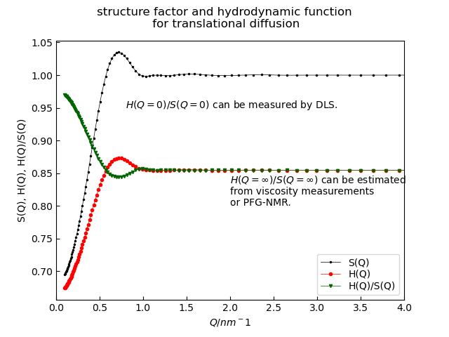
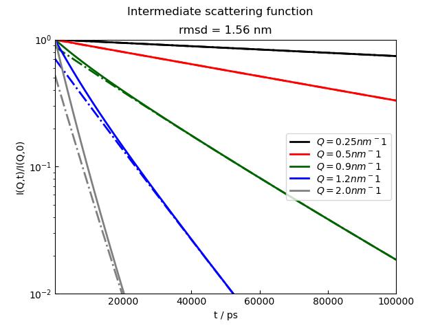
12.7.4. Load trajectory from MD simulation
A scatteringUniverse with a complete trajectory from MD simulation is created. The PSF needs atomic types to be guessed from names to identify atoms in the used format. You may need to install MDAnalysisTests to get the files.( python -m pip install MDAnalysisTests)
It might be necessary to transform the box that the protein is not crossing boundaries of the universe box.
from MDAnalysisTests.datafiles import PSF, DCD
import jscatter as js
import numpy as np
import MDAnalysis as mda
from MDAnalysis.topology.guessers import guess_types

upsf1 = js.bio.scatteringUniverse(PSF, DCD, assignTypes={'from_names':1})
upsf1.view(frames="all")

upsf1.setSolvent('1d2o1')
upsf1.qlist = js.loglist(0.1, 5, 100)

Sqtraj = js.dL()

# select protein and not the solvent if this is present
protein = upsf1.select_atoms('protein')

if 0:
    # only if needed to avoid crossing boundaries
    # add a transform that puts the protein into the center of the box and wrap the solvent into the new box
    # for details see  MDAnalysis Trajectory transformations
    protein = upsf1.select_atoms('protein')
    not_protein = upsf1.select_atoms('not protein')
    transforms = [trans.unwrap(protein),
                  trans.center_in_box(protein, wrap=True),
                  trans.wrap(not_protein, compound='fragments')]

# now loop over trajectory
for ts in upsf1.trajectory[2::13]:
    Sq = js.bio.nscatIntUniv(protein)
    Sq.time = upsf1.trajectory.time
    print(Sq.RgInt)
    Sqtraj.append(Sq)

# show
p = js.grace()
p.title('N scattering along ADK trajectory')
p.subtitle(r'change in R\sg\N; no change of SES volume')
p.yaxis(scale='l',label=r'I(Q) / nm\S2\N/particle')
p.xaxis(scale='l',label='Q / nm\S-1')
p.plot(Sqtraj,le=r't= $time ps; R\sg\N=$RgInt nm; V\sSES\N=$SESVolume nm\S3')
p.legend(x=0.15,y=1e-5,charsize=0.7)
# p.save(js.examples.imagepath+'/uniformfactorstraj.jpg', size=(2, 2))
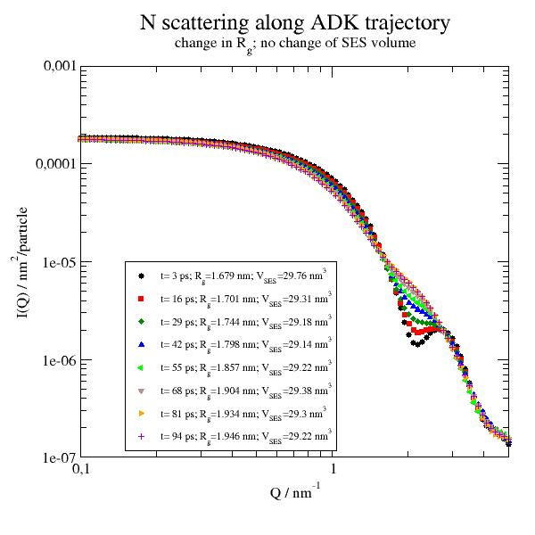
12.7.5. Compare different resolution options for coarse graining
PDB structures without explicit solvent for small angle scattering.
The example shows the validity of residue coarse graining up to around 3/nm. With coarse graining in cubes (cubesize) the approximation seems best. This might be useful to speed up computations that take long (e.g. ISF at low Q)
There is basically no difference between precalculated and averaged residue formfactors and explicit calculated residue formfactors for each residue (uni.explicitResidueFormFactorAmpl = True) The explicit ones include better deuteration of specific atoms.
Cα models loose some precision in volume respectively in forward scattering. C-alpha models need a .calphaCoarseGrainRadius = 0.342 nm because of the missing atoms. In addition, the mean residue position is not the C-alpha position. We use 0.342 nm as a good average to get same forward scattering over a bunch of proteins (see example_bio_proteinCoarseGrainRadius.py).
import jscatter as js

# first get and create the biological unit ('.pdb1') of alcohol dehydrogenase (tetramer, 144 kDa)
adh = js.bio.fetch_pdb('4w6z.pdb1')
# the 2 dimers in are in model 1 and 2 and need to be merged into one.
adhmerged = js.bio.mergePDBModel(adh)

# Ribonuclease A and Phosphoglycerate kinase are monomers and can be used without modifications.
# 3pgk has a Mg atom that is misinterpreted (as M), to use it we add this
vdwradii = {'M': js.data.vdwradii['Mg'] * 10}  # in A

p = js.grace(1, 1.4)
p.multi(3, 2, vgap=0, hgap=0)
for c, pdbid in enumerate(['3rn3', '3pgk', adhmerged]):
    # load from pdb id, scatteringUniverse adds hydrogens automatically
    uni = js.bio.scatteringUniverse(pdbid, vdwradii=vdwradii)
    uni.setSolvent('1d2o1')
    uni.qlist = js.loglist(0.1, 9.9, 200)
    u = uni.select_atoms("protein")
    ur = u.residues

    S = js.bio.nscatIntUniv(u)
    Sx = js.bio.xscatIntUniv(u)

    # use an averaging in cubes filled with the atoms, cubesize approximates residue size
    Scu = js.bio.nscatIntUniv(u, cubesize=0.6)
    Sxcu = js.bio.xscatIntUniv(u, cubesize=0.6)

    # use now the precalculated formfactors on residue level coarse graining
    uni.explicitResidueFormFactorAmpl = False  # default
    Sr = js.bio.nscatIntUniv(ur)
    Sxr = js.bio.xscatIntUniv(ur)

    # calc residue formfactors explicit (not precalculated)
    # useful for changes of residue deuteration or backbone N-H exchange of IDP
    uni.explicitResidueFormFactorAmpl = True
    Ser = js.bio.nscatIntUniv(ur)
    Sxer = js.bio.xscatIntUniv(ur)

    # create a C-alpha pdb file and then the Ca-only universe for calculation
    ca = uni.select_atoms('name CA')
    ca.write('pdb_ca.pdb')
    # addHydrogen=False prevents addition of 4H per C atom
    unica = js.bio.scatteringUniverse('pdb_ca.pdb', addHydrogen=False)
    # To use precalculated residue formfactors explicit... should be False
    unica.explicitResidueFormFactorAmpl = False
    unica.setSolvent('1d2o1')
    unica.qlist = js.loglist(0.1, 10, 200)
    uca = unica.residues
    Sca = js.bio.nscatIntUniv(uca, getVolume='now')
    Sxca = js.bio.xscatIntUniv(uca)

    p[2 * c].plot(S, li=[1, 2, 1], sy=0, le='atomic')
    p[2 * c].plot(Scu, li=[1, 2, 5], sy=0, le='atomic in cubes')
    p[2 * c].plot(Sr, li=[1, 2, 2], sy=0, le='res pre')
    p[2 * c].plot(Ser, li=[3, 2, 3], sy=0, le='res ex')
    p[2 * c].plot(Sca, li=[1, 2, 4], sy=0, le='Ca model')
    p[2 * c].legend(x=1, y=8e-3, charsize=0.8)
    p[2 * c].text(x=0.15, y=1e-7, charsize=1, string=pdbid)

    p[2 * c + 1].plot(Sx, li=[1, 2, 1], sy=0, le='atomic')
    p[2 * c + 1].plot(Sxcu, li=[1, 2, 5], sy=0, le='atomic in cubes')
    p[2 * c + 1].plot(Sxr, li=[1, 2, 2], sy=0, le='res pre')
    p[2 * c + 1].plot(Sxer, li=[3, 2, 3], sy=0, le='res ex')
    p[2 * c + 1].plot(Sxca, li=[1, 2, 4], sy=0, le='Ca model')
    p[2 * c + 1].legend(x=1, y=8e-3, charsize=0.8)
    p[2 * c + 1].text(x=0.15, y=1e-7, charsize=1, string=pdbid)

    p[2 * c].xaxis(label='', ticklabel=False, scale='log', min=1e-1, max=9.9)
    p[2 * c + 1].xaxis(label='', ticklabel=False, scale='log', min=1e-1, max=9.9)
    p[2 * c].yaxis(label='F(Q)', ticklabel='power', scale='log', min=3e-8, max=8e-3)
    p[2 * c + 1].yaxis(ticklabel=False, scale='log', min=3e-8, max=8e-3)

p[2 * c].xaxis(label=r'Q / nm\S-1', ticklabel=True, scale='log', min=1e-1, max=9.9)
p[2 * c + 1].xaxis(label=r'Q / nm\S-1', ticklabel=True, scale='log', min=1e-1, max=9.9)
p[0].subtitle('neutron scattering')
p[1].subtitle('Xray scattering')
p[0].title(' ' * 30 + 'Comparison of formfactors with different resolution')
# p.save(js.examples.imagepath+r'/uniformfactors.jpg', size=(700/300, 1000/300))
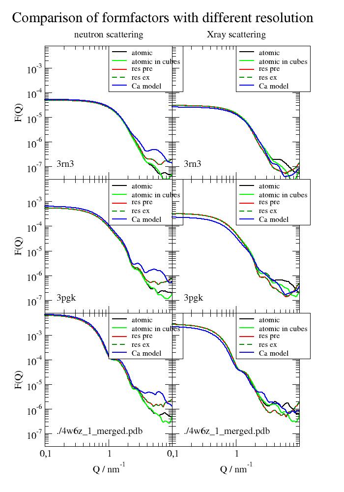
12.7.6. Selective partial deuteration
Partial deuteration of protein complexes is a promising tool for examination of protein structure function relationship. E.g. see an interesting example about the complex in the cyanobacterial circadian clock system Sugiyama et al, Nature Communications Biology (2022). https://doi.org/10.1038/s42003-022-03143-z
Here we see how to selectively deuterate domains or specific aminoacids and how scattering is influenced. The deuteration is considered in all bio methods.
import jscatter as js
import numpy as np
import scipy.constants as constants

# create universe
mab = js.bio.scatteringUniverse('1igt')
mab.setSolvent('1d2o1')

mab.qlist = np.r_[0.01, 0.1:4:0.03]
# use explicit residue formfactors for EACH residue
mab.explicitResidueFormFactorAmpl = True

# use a atom selection
lightchains = mab.select_atoms('segid A C')  # light chains

mab.atoms.deuteration = 0  # default protonated
I_protonated = js.bio.nscatIntUniv(mab.atoms)

lightchains.atoms.deuteration = 1
I_lightdeuterated = js.bio.nscatIntUniv(mab.atoms)

mab.atoms.deuteration = 0
# select fc domain
mab.select_atoms('segid B D and resid 240-700').deuteration = 1
I_fcdeuterated = js.bio.nscatIntUniv(mab.atoms)

mab.atoms.deuteration = 0
# select 3 residue
mab.select_atoms('resname ALA ARG ASN ').deuteration = 1
I_someAA = js.bio.nscatIntUniv(mab.atoms)
#

I_someresidue = js.bio.nscatIntUniv(mab.residues)

p = js.grace()
p[0].plot(I_protonated, sy=0, li=[1, 3, 1], le='full protonated')
p[0].plot(I_lightdeuterated, sy=0, li=[1, 3, 2], le='light chain deuterated')
p[0].plot(I_fcdeuterated, sy=0, li=[1, 3, 3], le='fc domain deuterated')
p[0].plot(I_someAA, sy=0, li=[1, 3, 4], le='ALA ARG ASN deuterated')
p[0].plot(I_someresidue, sy=0, li=[3, 3, 5], le='ALA ARG ASN deuterated coarse grain')


p.xaxis(label=r'Q / nm\S-1', min=0, max=4)
p.yaxis(label=r'I(Q) / 1/cm', scale='log', min=1e-6, max=0.01)
p.legend(x=1, y=0.008)
p.title('selective protein deuteration')

# p.save('bio_protein_partialmatching.png')
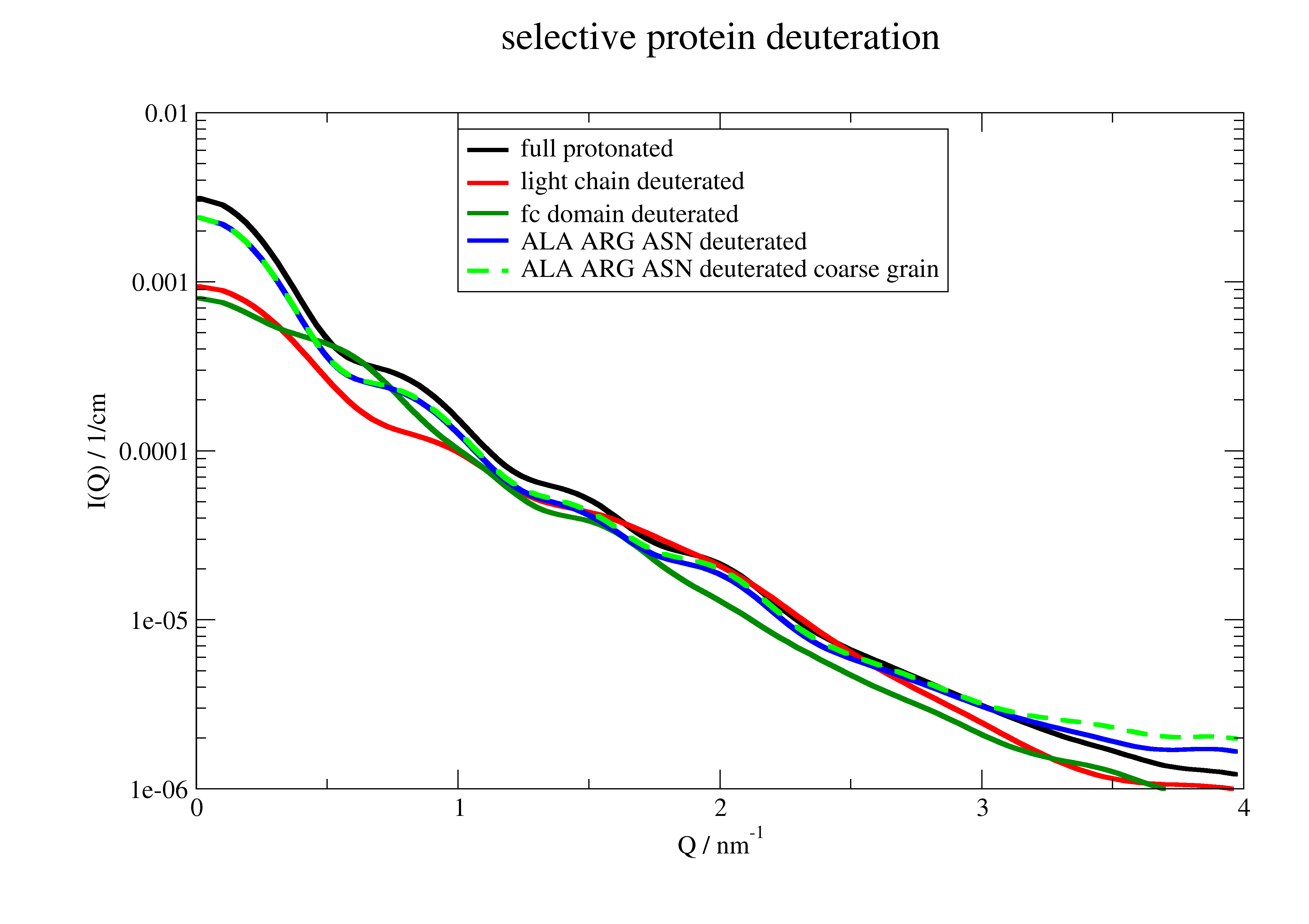
12.7.7. A protein normal mode animation
Creating a trajectory from normal modes and show I(Q) together with the configuration.
The calculation can also be done along a MD simulation in .trajectory .
MDAnalysis allows a bunch of trajectory manipulations like center of mass removal or rotations.
import jscatter as js
import numpy as np
import tempfile
import os
import pymol2
import matplotlib.image as mpimg


def savepng(u, fname):
    """Save png image from pymol"""
    p1 = pymol2.PyMOL()
    p1.start()
    with tempfile.TemporaryDirectory() as tdir:
        name = os.path.splitext(u.filename)[0] + '.pdb'
        tfile = os.path.join(tdir, name)
        u.atoms.write(tfile)
        p1.cmd.load(tfile)
        p1.cmd.rotate('x', 90, 'all')
        p1.cmd.color('red', 'ss h')
        p1.cmd.color('yellow', 'ss s')
        p1.cmd.color('blue', 'ss l+')
        p1.cmd.set('cartoon_discrete_colors',1)
        p1.cmd.png(fname, width=600, height=600, dpi=-1, ray=1)
    p1.stop()


uni=js.bio.scatteringUniverse(js.examples.datapath+'/arg61.pdb', addHydrogen=False)

uni=js.bio.scatteringUniverse('3pgk')
uni.setSolvent('1d2o1')
u = uni.select_atoms("protein and name CA")
# create normal modes
nm = js.bio.vibNM(u)
# make a trajectory similar to a MD simulation
moving = nm.animate([6,7,8,9], scale=120)
moving.qlist = js.loglist(0.1, 5, 100)

p = js.mplot(16, 8)
# loop over trajectory timesteps
for i, ts in enumerate(moving.trajectory):
    # calc th scattering and plot it
    Sq = js.bio.xscatIntUniv(moving.atoms, refreshVolume=False)
    p.Multi(1, 2)
    p[1].axis('off')
    p[0].Plot(Sq, li=[1,2,1], sy=0)
    p[0].Yaxis(label='F(Q) / nm²', scale='log', min=3e-7, max=6e-4)
    p[0].Xaxis(label=r'$Q / nm^{-1}$')
    name = f'test_{i:.0f}.png'
    savepng(moving, name)
    img = mpimg.imread(name)
    p[1].imshow(img)
    # p.savefig(name, transparent=True, dpi=100)
    p.clear()

p.Close()

# In Ipython use ImageMagic to generate animated gif
# %system convert -delay 10 -loop 0  -dispose Background test*.png mode_animation.gif
12.7.8. Protein density determination
We compare measured protein density data with the density calculated by Jscatter
to check the SESVolume accuracy in the module jscatter.bio .
Respective references are given in js.examples.datapath+'/proteinSpecificVolumes.txt'
import os.path
import jscatter as js
import numpy as np

# Comparison of the calculated protein density with several references

# read partial specific volumes
with open(js.examples.datapath+'/proteinSpecificVolumes.txt') as f:
    lines = f.readlines()

universes = []
for line in lines:
    words = line.split()
    if len(words)==0 or words[0].startswith('#'):
        continue
    print(words)
    author = words[3]
    if os.path.exists(words[1]+'_h.pdb'):
        uni = js.bio.scatteringUniverse(words[1]+'_h.pdb', addHydrogen=False)
    else:
        uni = js.bio.scatteringUniverse(words[1])
    uni.densityPaper= 1/float(words[2])
    uni.qlist = js.loglist(0.1, 4, 40)
    uni.solvent = ['0D2O1', '1H2O1']
    uni.pdb = words[1]
    uni.author = author
    universes.append(uni)

Slist = js.dL()
for uni in universes:
    uni.probe_radius = 0.13
    u = uni.select_atoms("protein")
    S = js.bio.scatIntUniv(u, mode='xray')
    S.densityPaper = uni.densityPaper
    S.author = uni.author
    Slist.append(S)

p=js.grace()
p.plot(Slist.mass.array/1000., Slist.massdensity, sy=[1, 0.5, 1, 1], le='Jscatter')
for c, author in enumerate(Slist.author.unique, 2):
    Sl = Slist.filter(author=author)
    p.plot(Sl.mass.array/1000., Sl.densityPaper.array, sy=[c, 0.5, c], le=author)
dev = Slist.massdensity/Slist.densityPaper.array
p.xaxis(min=3, max=600, label=r'molecular weight / kDa', charsize=1.5, scale='log')
p.yaxis(label=r'density / g/cm\S3\N', charsize=1.5)
st = fr'Mean density {Slist.densityPaper.mean:.2f}+-{Slist.densityPaper.std:.2f} g/cm\S3\N;' \
      +fr' Jscatter deviation  {dev.mean():.3f}+-{dev.std():.3f}'
p.subtitle(st)
p.title(r'Comparing Jscatter protein density with references ')
p.legend(x=100, y=1.45)
# p.save('proteinDensityTest.png')
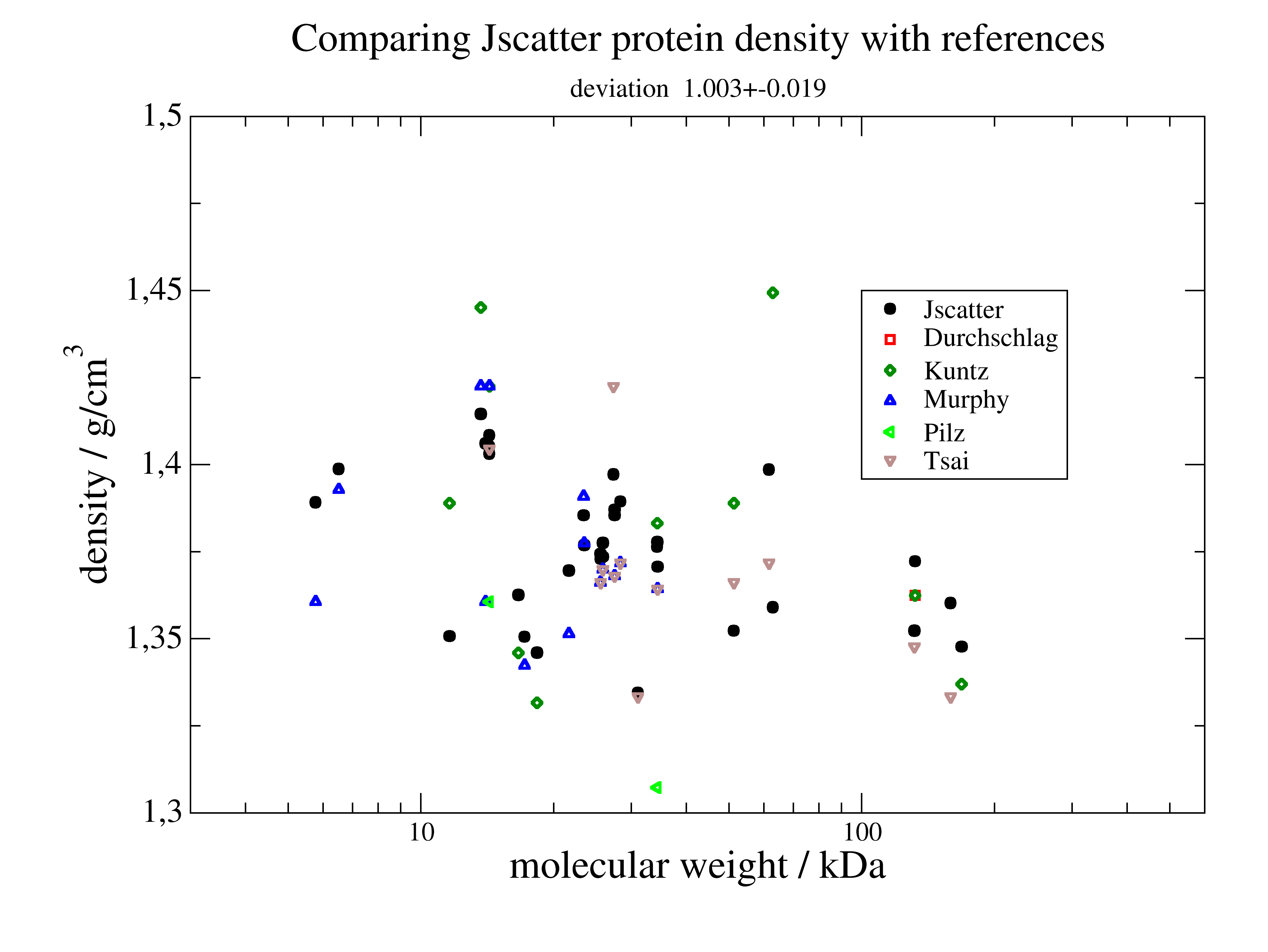
12.7.9. Cα coarse grain radius
We calculate an appropriate Size of residues dummy atoms for Cα atom models to get a reasonable protein scattering intensity.
"""
This test determines the best calphaCoarseGrainRadius to result in
best approximated forward scattering I0 of the selected proteins.

The best result is for calphaCoarseGrainRadius = 0.362

Dependent on the protein structure slightly different values might be better.
But anyway bead models and Cα models are always a rough approximation.

"""
import jscatter as js
import numpy as np
import os

with open(js.examples.datapath + '/proteinSpecificVolumes.txt') as f:
    lines = f.readlines()

vdw = {'CO': 0.15, 'Z': js.data.vdwradii['Zn'] * 10, 'M': js.data.vdwradii['Mg'] * 10}

Slist = js.dL()
for line in lines:
    words = line.split()
    if len(words)==0 or words[0].startswith('#'):
        continue
    if len(Slist)>0 and words[1] in Slist.proteinID:
        continue
    if os.path.exists(words[1]+'_h.pdb'):
        uni = js.bio.scatteringUniverse(words[1]+'_h.pdb', addHydrogen=False)
    else:
        uni = js.bio.scatteringUniverse(words[1])
    u = uni.select_atoms("protein")
    S = js.bio.xscatIntUniv(u)
    ca = uni.select_atoms('name CA')
    ca.write('uniCA.pdb')
    unica = js.bio.scatteringUniverse('uniCA.pdb', addHydrogen=False)
    uca = unica.residues
    pr = np.r_[0.3:0.4:0.01]
    for r in pr:
        print(words[1], r)
        unica.calphaCoarseGrainRadius = r
        Sca = js.bio.xscatIntUniv(uca)
        Sca.relVolume = Sca.SESVolume / S.SESVolume
        Sca.relI0 = Sca.I0 / S.I0
        Sca.atomVolume = S.SESVolume
        Sca.proteinID = words[1]
        Sca.pr = r
        Slist.append(Sca)

p2 = js.grace()
p2.multi(1, 2)
xx = []
for id in Slist.proteinID.unique:
    sl = Slist.filter(proteinID=id)
    rV = js.dA(np.c_[sl.pr, sl.relI0].T)
    rV.fit(lambda x, b, x0: (b * (x - x0) + 1) ** 2, {'b': 11, 'x0': 0.35}, {}, {'x': 'X'})
    p2[0].plot(rV, le=f'{rV.x0:.3f}')
    p2[0].plot(rV.lastfit, li=[1,0.3,11])
    p2[1].plot([sl[0].mass], [rV.x0])
    xx.append(rV.x0)
xx = np.array(xx)
p2[0].plot([0.1, 0.4], [1] * 2, sy=0, li=1)
p2[0].xaxis(label='Ca radius / nm', min=0.28, max=0.45)
p2[0].yaxis(label='relative intensity')
p2[1].xaxis(scale='log', label='mass / Da')
p2[1].yaxis(label=['best Ca radius / nm',1,'opposite'],ticklabel= ['general',2,1,'opposite'])
p2[1].subtitle(f'best Ca CG radius = {np.mean(xx):.3f} +- {np.std(xx):.3f} ')
p2[0].title('                            Determination of best Ca coarse grain radius')
# p2.save('proteinCacoarsegrainRadius.png')

# Conclusion CA model with vdWradius 0.342 is appropriate
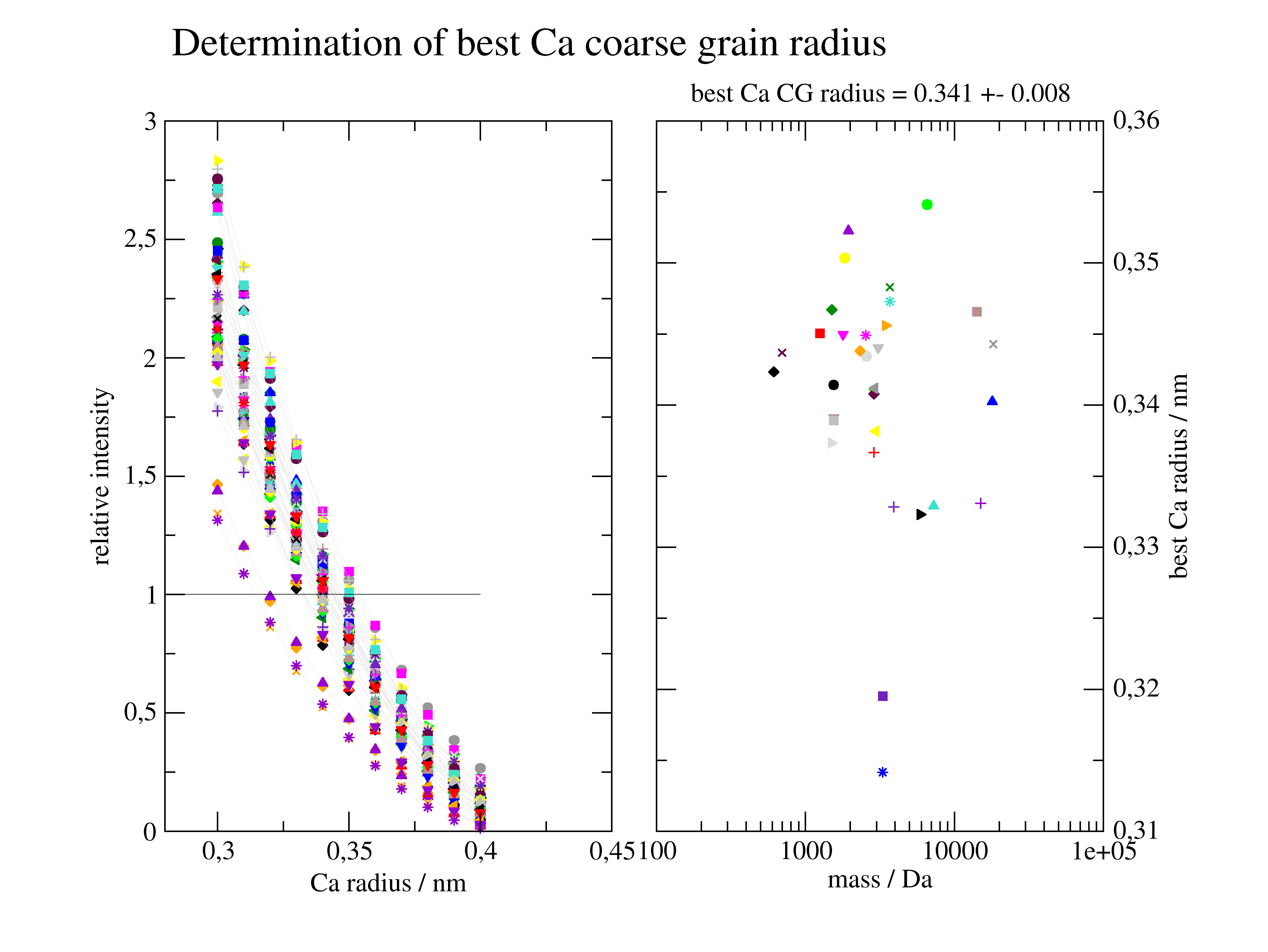
12.8. Other stuff
12.8.1. Sedimentation of two particle sizes and resulting scattering: a Simulation
# The question is how long do I need to centrifuge to get rid of
# the larger aggregates and not just guess somewhat.

import numpy as np
import jscatter as js

t1 = np.r_[100:2e3:11j]  # time in seconds

# open plot()
p = js.grace(1.5, 1.5)
p[0].SetView(0.15, 0.12, 0.9, 0.85)
# calculate sedimentation profile for two different particles
# data correspond to Fresco 21 with dual rotor
# default is solvent='h2o',temp=293
Rh1 = 2  # nm
Rh2 = 40  # nm
g = 21000.  # g # RZB number
omega = g * 246 / 21000
profiles1 = js.formel.sedimentationProfile(t=t1, Rh=Rh1, c0=0.05, omega=omega, rm=48, rb=85)
profiles2 = js.formel.sedimentationProfile(t=t1, Rh=Rh2, c0=0.05, omega=omega, rm=48, rb=85)

# plot it
p.plot(profiles1, li=-1, sy=0, legend='%s nm -> t=$time s' % Rh1)
p.plot(profiles2, li=[2, 2, -1], sy=0, legend='%s nm-> t=$time s' % Rh2)

# label the plot with some explanations
p.title(r'sedimentation of %s nm species and %s nm species \nafter t seconds centrifugation ' % (Rh1, Rh2), size=1)
p.subtitle(r'rotor speed %s rps=%sg, r\smeniscus\N=48mm, r\sbottom\N=85mm' % (omega, g))
p.yaxis(max=0.2, min=0, label='concentration')
p.xaxis(label='position in cell / mm')
p.legend(x=40, y=0.2, charsize=0.5)
p.text(r'%s nm particles \nnearly not sedimented \nin sedimentation time of %s nm' % (Rh1, Rh2), 44, 0.07)
p.text(r'%snm sediment\nquite fast' % Rh2, 73, 0.105)
p[0].line(80, 0.1, 84, 0.08, 5, arrow=2)
p.save('CentrifugationProfiles.png')
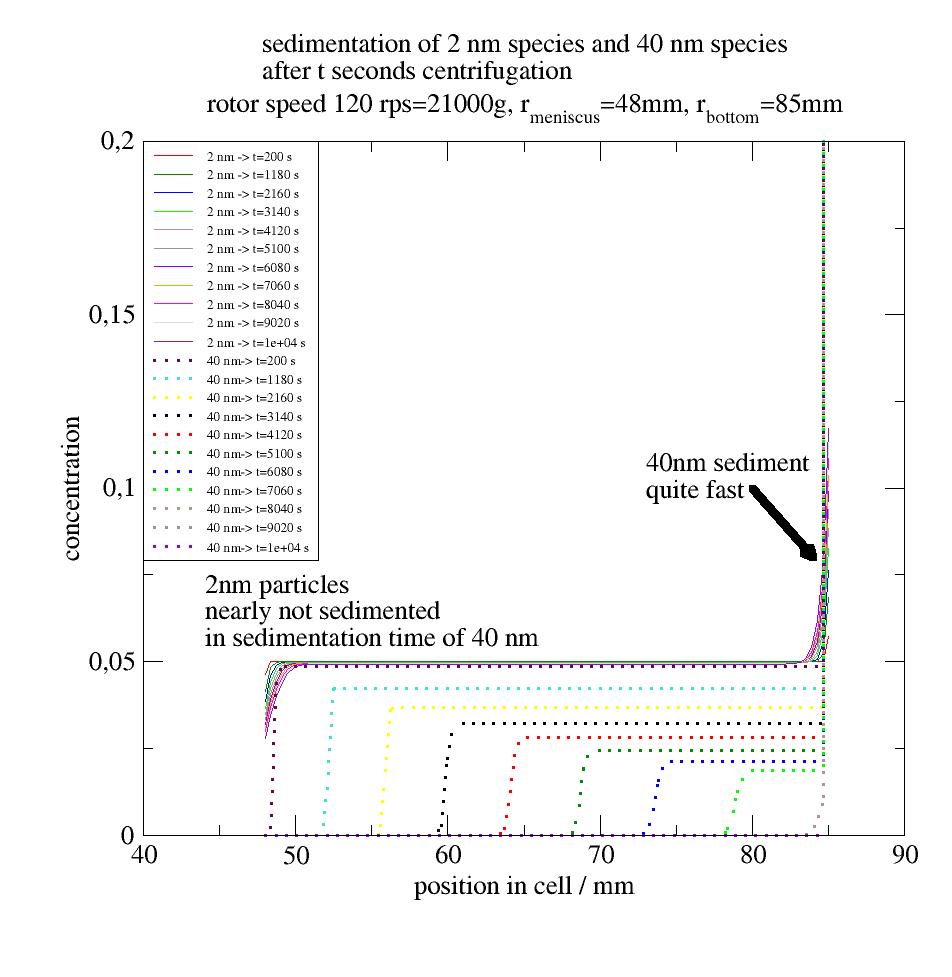
# corresponding small angle scattering for the above
# centrifugation is done to remove the large fraction
# how long do you need to centrifuge and how does it look without centrifugation?
# scattering for a 2 nm particle and 40 nm particle with same intensity in DLS
# with DLS you can see easily the aggregates

p = js.grace()
# equal intensity  of both species in DLS as in SANS
p.plot(js.formel.scatteringFromSizeDistribution(js.loglist(1e-2, 4, 100), [[Rh1, Rh2], [1, 1]], func=js.ff.beaucage))
# larger has 10% of smaller species intensity
p.plot(js.formel.scatteringFromSizeDistribution(js.loglist(1e-2, 4, 100), [[Rh1, Rh2], [1, 0.1]], func=js.ff.beaucage))
# larger species particles
p.plot(js.formel.scatteringFromSizeDistribution(js.loglist(1e-2, 4, 100), [[Rh1, Rh2], [1, 0]], func=js.ff.beaucage))

p.xaxis(min=0.01, max=5, scale='l', label=r'Q / nm\S-1')
p.yaxis(min=0, max=2, label='I(Q)')
p.title('How does %.2g nm aggregates influence SANS scattering' % Rh2, size=1)
p.subtitle('Beaucage form factor with d=3 for spherical particles')
p.text('Here Rg is determined', x=0.2, y=1)
p.text(r'10%% intensity as\n %.2g nm in DLS' % Rh1, x=0.011, y=1.2)
p.text(r'same intensity as\n %.2g nm in DLS' % Rh1, x=0.02, y=1.9)
p.text('no big aggregates', x=0.011, y=0.9)
p.save('AggregtesinSANS.png')
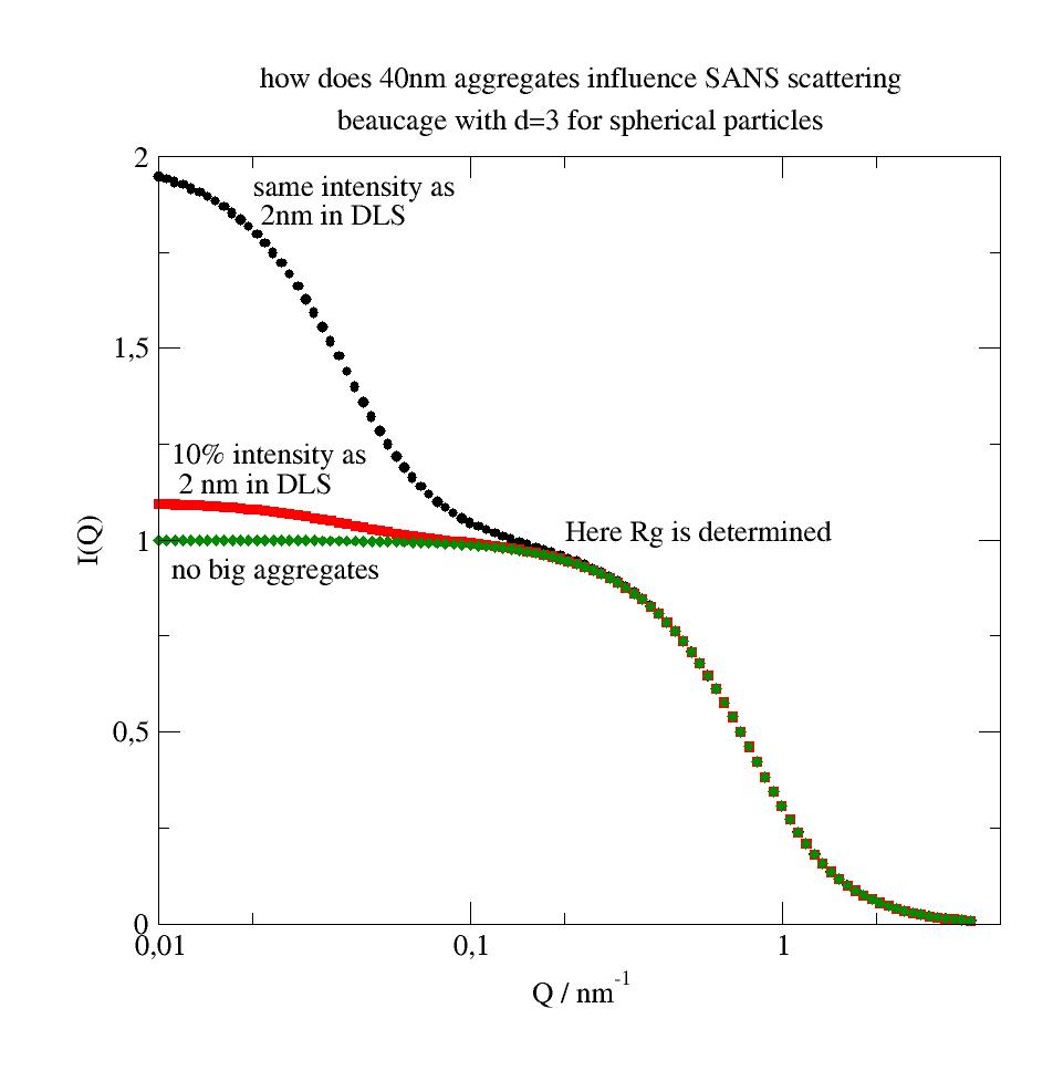
12.8.2. Create a stacked chart of some curves
import numpy as np
import jscatter as js

# create a stacked chart of 10 plots

# create some data
mean = 5
x = np.r_[mean - 3 * 3:mean + 3 * 3:200j]
data = js.dL()  # empty dataList
for sigma in np.r_[3:0.3:10j]:
    temp = js.dA(np.c_[x, np.exp(-0.5 * (x - mean) ** 2 / sigma ** 2) / sigma / np.sqrt(2 * np.pi)].T)
    temp.sigma = sigma
    data.append(temp)

p = js.grace()
# each shifted by hshift,vshift
# the yaxis is switched off for all except the first
p.stacked(10, hshift=0.02, vshift=0.01, yaxis='off')
# plot some Gaussians in each graph
for i, dat in enumerate(data):
    p[i].plot(dat, li=[1, 2, i + 1], sy=0, legend='sigma=$sigma')
# choose the same yscale for the data but no ticks for the later plots
# adjusting the scale and the size of the xaxis ticks

p[0].yaxis(min=0, max=1, tick=[0.2, 5, 0.3, 0.1])
p[0].xaxis(min=min(x), max=max(x), tick=[1, 1, 0.3, 0.1])
for pp in p.g[1:]:
    pp.yaxis(min=0, max=1, tick=False)
    pp.xaxis(min=min(x), max=max(x), tick=[1, 1, 0.3, 0.1])

# This plot is shown below; no fine tuning
if 1:
    p.save('stackedGaussians.agr')
    p.save('stackedGaussians', format='jpeg')

# change the stacking to improve plot (or not)
p.stacked(10, hshift=-0.015, vshift=-0.01, yaxis='off')
p.title('stacked')
# create a plot with exponential decaying function but shifted consecutively by factors of 2
x = js.loglist(0.01, 5, 100)
p = js.grace()
for i in np.r_[1:10]:
    p.plot(x, np.exp(-i ** 2 * x ** 2))

p.shiftbyfactor(xfactors=2 * np.r_[10:1:-1], yfactors=2 * np.r_[10:1:-1])
p.yaxis(scale='l')
p.xaxis(scale='l')
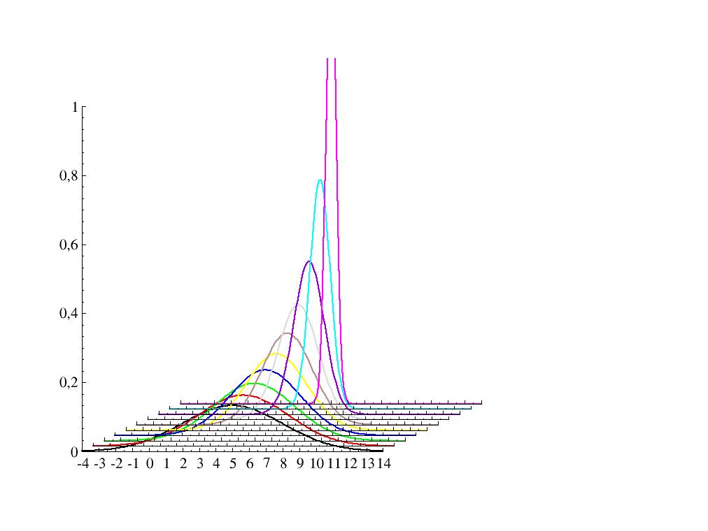
Some examples to show how to use Jscatter.
Functions show the code or run the examples in example directory.
- jscatter.examples.showExampleList()[source]
Show an updated list of all examples.
Currently, availible examples
    0  example_2D_EwaldSphere.py
1  example_2D_orientedScattering.py
2  example_2D_structurefactors.py
3  example_BG_2DFitting.py
4  example_BG_2DFitting_CrystalPeaks.py
5  example_BG_SinusoidalFitting.py
6  example_BG_SinusoidalFitting_linkedParameter.py
7  example_BG_buildComplexModel.py
8  example_BG_buildsimpleModels.py
9  example_BG_cloudscattering.py
10  example_BG_fit_Regularisation.py
11  example_BG_fit_bayes.py
12  example_BG_fit_diffusion.py
13  example_BG_fit_multicylinder.py
14  example_BG_fit_regularizedEM.py
15  example_BG_simple_diffusion.py
16  example_CONTIN.py
17  example_CONTIN_weights.py
18  example_Sedimentation.py
19  example_StructureFactors.py
20  example_TeubnerStrey.py
21  example_Zimm.py
22  example_bio_comparecoarsegraining.py
23  example_bio_loadPDB.py
24  example_bio_loadTrajectory.py
25  example_bio_makeNManimation.py
26  example_bio_partialdeuteratedprotein.py
27  example_bio_proteinCoarseGrainRadius.py
28  example_bio_proteinNormalModesScattering.py
29  example_bio_proteinNormalModesScattering_2.py
30  example_bio_proteinVolume.py
31  example_bio_proteinformfactoranddiffusion.py
32  example_bio_trajectoryAnalysis.py
33  example_daily_use.py
34  example_dy_HydrodynamicFunction.py
35  example_dy_collectiveZimmDynamics.py
36  example_dy_dynamics.py
37  example_dy_fitTime+FrequDomain.py
38  example_dy_fit_InelasticInstrument_simple.py
39  example_dy_fit_differentInelasticInstruments.py
40  example_dy_inelasticNeutronScattering.py
41  example_grace0_newsimplestyle.py
42  example_grace1.py
43  example_grace2.py
44  example_grace3.py
45  example_grace_stackeddata.py
46  example_hexagonalLatticeofCylinders1.py
47  example_hexagonalLatticeofCylinders2.py
48  example_interfacialBicelleModel.py
49  example_makeJ.py
50  example_membraneStack.py
51  example_orientedCloudCube.py
52  example_sas_MultipleContrastFit.py
53  example_sas_SANSsmearing.py
54  example_sas_SASdesmearing.py
55  example_sas_analyseSASData.py
56  example_sas_comparisonLattices.py
57  example_sas_connected_linearPearls.py
58  example_sas_fitwithsmearing.py
59  example_sas_multilamellarVesicle.py
60  example_sas_multilamellarVesicleSAXS.py
61  example_sas_multilamellarVesiclereal.py
62  example_sas_smooth_xraydata.py
- jscatter.examples.runExample(example, usempl=False)[source]
Run example by number or name.
Example and saved files go to JscatterExamples/example_name in the current working directory.
- Parameters:
- example: string,int
Filename or number of the example to run
- usemplbool, default False
For using mpl set to True
Examples
import jscatter as js js.examples.runExample(‘daily_use’)