Fitting 1D, 2D 3D …

1D fits with attributes

Some Sinusoidal fits with different kinds to use dataArray attributes. We use dataArray for fitting.

# Basic fit examples with synthetic data. Usually data are loaded from a file.

import jscatter as js
import numpy as np

sinus = lambda x, A, a, B: A * np.sin(a * x) + B  # define model

# Fit sine to simulated data
x = np.r_[0:10:0.1]
data = js.dA(np.c_[x, np.sin(x) + 0.2 * np.random.randn(len(x)), x * 0 + 0.2].T)  # simulate data with error
data.fit(sinus, {'A': 1.2, 'a': 1.2, 'B': 0}, {}, {'x': 'X'})  # fit data
data.showlastErrPlot()  # show fit
data.errPlotTitle('Fit Sine')

# Fit sine to simulated data using an attribute in data with same name
data = js.dA(np.c_[x, 1.234 * np.sin(x) + 0.1 * np.random.randn(len(x)), x * 0 + 0.1].T)  # create data
data.A = 1.234  # add attribute
data.makeErrPlot()  # makes errorPlot prior to fit
data.fit(sinus, {'a': 1.2, 'B': 0}, {}, {'x': 'X'})  # fit using .A
data.errPlotTitle('Fit Sine with attribute')

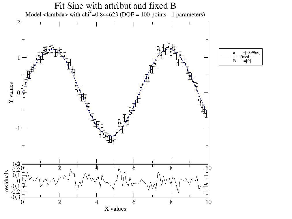
# Fit sine to simulated data using an attribute in data with different name and fixed B
data = js.dA(np.c_[x, 1.234 * np.sin(x) + 0.1 * np.random.randn(len(x)), x * 0 + 0.1].T)  # create data
data.dd = 1.234  # add attribute
data.fit(sinus, {'a': 1.2, }, {'B': 0}, {'x': 'X', 'A': 'dd'})  # fit data
data.showlastErrPlot()  # show fit
data.errPlotTitle('Fit Sine with attribute and fixed B')

2D fit with attributes

A 2D fit using the attribute B stored in the dataArray of a dataList as second dimension.

We use dataList for fitting. This might be extended to several attributes allowing multidimensional fitting. See also Simple diffusion fit of not so simple diffusion case

# Fit sine to simulated dataList using an attribute in data with different name
# and fixed B from data.
# first one common parameter then as parameter list
# create data
data = js.dL()
ef = 0.1  # increase this to increase error bars of final result
for ff in [0.001, 0.4, 0.8, 1.2, 1.6]:
    data.append(js.dA(np.c_[x, (1.234 + ff) * np.sin(x + ff) + ef * ff * np.random.randn(len(x)), x * 0 + ef * ff].T))
    data[-1].B = 0.2 * ff / 2  # add attributes

# fit with a single parameter for all data, obviously wrong result
data.fit(lambda x, A, a, B, p: A * np.sin(a * x + p) + B, {'a': 1.2, 'p': 0, 'A': 1.2}, {}, {'x': 'X'})
data.showlastErrPlot()  # show fit
data.errPlotTitle('Fit Sine with attribute and common fit parameter')

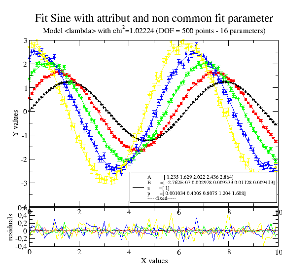
# now allowing multiple p,A,B as indicated by the list starting value
data.fit(lambda x, A, a, B, p: A * np.sin(a * x + p) + B, {'a': 1.2, 'p': [0], 'B': [0, 0.1], 'A': [1]}, {}, {'x': 'X'})
data.errPlotTitle('Fit Sine with attribute and non common fit parameter')

# plot p against A , just as demonstration
p = js.grace()
p.plot(data.A, data.p, data.p_err, sy=[1, 0.3, 1])
p.xaxis(label='Amplitude')
p.yaxis(label='phase')

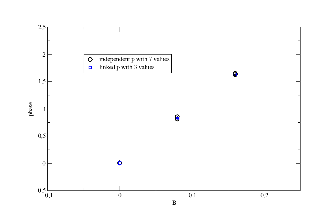
2D fit with attributes and linked parameter

A 2D fit as above but the fit parameter is linked to the attribute B that apears several times with the same value. In experimental data this might be a repeated measurement with a different intensity for the same process.

We get only as many fit parameters as we have unique values for B (here 3 different values).

Important is to link by adding ‘B’ in {..., 'p':[0, 'B'], ...} to the list of starting values.

#
import jscatter as js
import numpy as np

# create data. B will appear several times with same value
data = js.dL()
x = np.r_[0:10:0.1]
ef = 0.1  # increase this to increase error bars of final result
for ff in [0.001, 0.8, 1.6]:
    data.append(js.dA(np.c_[x, (1.234 + ff) * np.sin(x + ff) + ef * ff * np.random.randn(len(x)), x * 0 + ef * ff].T))
    data[-1].B = 0.2 * ff / 2  # add attributes
    # add same but different amplitude A, same phase p
    data.append(js.dA(np.c_[x, (0.234 + ff) * np.sin(x + ff) + ef * ff * np.random.randn(len(x)), x * 0 + ef * ff].T))
    data[-1].B = 0.2 * ff / 2  # add attributes

data.append(js.dA(np.c_[x, (0.234 + ff) * np.sin(x + ff) + ef * ff * np.random.randn(len(x)), x * 0 + ef * ff].T))
data[-1].B = 0.2 * ff / 2  # add attributes


# create model
model = lambda x, A, a, B, p: A * np.sin(a * x + p) + B

# plot for result
p = js.grace()

# fit with independent parameters for all dataList elements
data.fit(model, {'a': 1.2, 'p': [0], 'A': [1.2]}, {}, {'x': 'X'})

# plot p against unique B
p.plot(data.B, data.p, data.p_err, sy=[1, 1, 1], legend='independent p with 7 values')

# now A still independent but we link 'p' to 'B'
data.fit(model, {'a': 1.2, 'p': [0, 'B'], 'A': [1]}, {}, {'x': 'X'})

# plot p against unique B with less values in p
p.plot(data.B.unique, data.p, data.p_err, sy=[2, 0.7, 4], le='linked p with 3 values')
p.xaxis(label='B', min=-0.1, max=0.25)
p.yaxis(label='phase',min=-0.5,max=2.5)
p.legend(x=-0.05,y=2)
p.save('SinusoidalFit_linkedParameter.png')

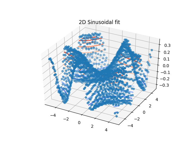
2D fitting using .X, .Z, .W

Unlike the previous we use here data with two dimensions in .X,.Z coordinates (optional .W for 3D). We use dataArray for fitting. Additional one could use again attributes to increase dimesion. This mainly depends on the data.

Another example is shown in Fitting the 2D scattering of a lattice.

import jscatter as js
import numpy as np

# 2D fit data with an X,Z grid data and Y values (For 3D we would use X,Z,W )
# For 2D fit we calc Y values from X,Z coordinates (only for scalar Y data).
# For fitting we need data with X,Z,Y columns indicated .

#  We create synthetic 2D data with X,Z axes and Y values as Y=f(X,Z)
# This is ONE way to make a grid. For fitting it can be unordered, non-gridded X,Z data
x, z = np.mgrid[-5:5:0.25, -5:5:0.25]
xyz = js.dA(np.c_[x.flatten(), z.flatten(), 0.3 * np.sin(x * z / np.pi).flatten() + 0.01 * np.random.randn(
    len(x.flatten())), 0.01 * np.ones_like(x).flatten()].T)
# set columns where to find X,Z coordinates and Y values and eY errors )
xyz.setColumnIndex(ix=0, iz=1, iy=2, iey=3)


# define model
def ff(x, z, a, b):
    return a * np.sin(b * x * z)


xyz.fit(model=ff, freepar={'a': 1, 'b': 1 / 3.}, fixpar={}, mapNames={'x': 'X', 'z': 'Z'})

# show in 2D plot
import matplotlib.pyplot as plt
from matplotlib import cm

fig = plt.figure()
ax = fig.add_subplot(111, projection='3d')
ax.set_title('2D Sinusoidal fit')
# plot data as points
ax.scatter(xyz.X, xyz.Z, xyz.Y)
# plot fit as contour lines
ax.tricontour(xyz.lastfit.X, xyz.lastfit.Z, xyz.lastfit.Y, cmap=cm.coolwarm, antialiased=False)
plt.show(block=False)

Simple diffusion fit of not so simple diffusion case

Here the long part with description from the first example.

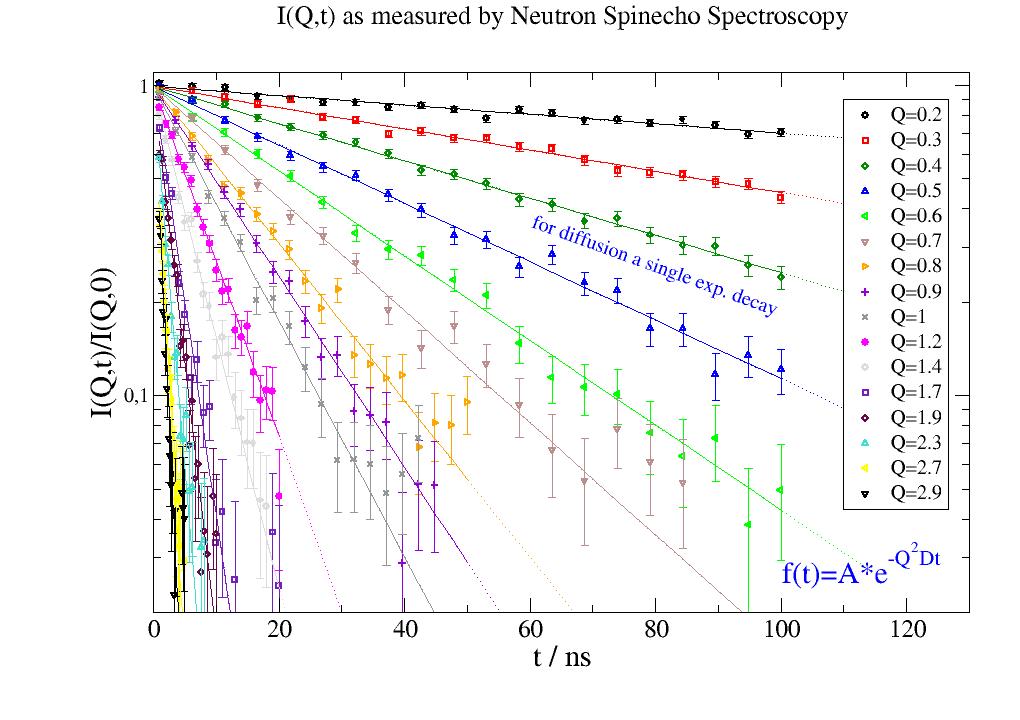
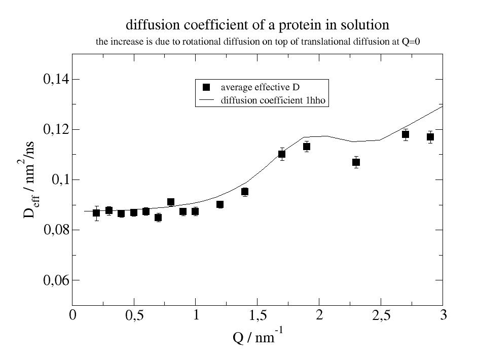
This is the diffusion of a protein in solution. This is NOT constant as for Einstein diffusion.

These simulated data are similar to data measured by Neutron Spinecho Spectroscopy, which measures on the length scale of the protein and therefore also rotational diffusion contributes to the signal. At low wavevectors additional the influence of the structure factor leads to an upturn, which is neglected in the simulated data. To include the correction \(D_T(q)=D_{T0} H(q)/S(q)\) look at hydrodynamicFunct().

For details see this tutorial review Biehl et al. Softmatter 7,1299 (2011)

A key point for a simultaneous combined fit is that each dataArray has an individual ‘q’ which is used in the fit model as ‘wavevector’.

# import jscatter and numpy
import numpy as np
import jscatter as js

# read the data (16 dataArrays) with attributes as q, Dtrans .... into dataList
i5 = js.dL(js.examples.datapath + '/iqt_1hho.dat')

# define a model for the fit
diffusion = lambda A, D, t, wavevector, e=0: A*np.exp(-wavevector**2*D*t) + e

# do the fit
# single valued start parameters are the same for all 16 dataArrays
# list start parameters [...] indicate independent fitting for dataArrays
# the command line shows progress and the final result, which is found in i5.lastfit
i5.fit(model=diffusion,                         # the fit function
       freepar={'D': [0.08], 'A': 0.98},        # free start parameters
       fixpar={'e': 0.0},                       # fixed parameters
       mapNames={'t': 'X', 'wavevector': 'q'})  # map names from model to data

# open plot with results and residuals
i5.showlastErrPlot(yscale='l')

# open a plot with fixed size and plot data and fit result
p = js.grace(1.2, 0.8)
# plot the data with Q values in legend as symbols
p.plot(i5, symbol=[-1, 0.4, -1], legend='Q=$q')
# plot fit results in lastfit as lines without symbol or legend
p.plot(i5.lastfit, symbol=0, line=[1, 1, -1])
# extend to longer times by changing a model parameter (points)
p.plot(i5.modelValues(t=np.r_[10:120:5]), symbol=0, line=[2, 1, -1])

# pretty up if needed
p.yaxis(min=0.02, max=1.1, scale='log', charsize=1.5, label='I(Q,t)/I(Q,0)')
p.xaxis(min=0, max=130, charsize=1.5, label='t / ns')
p.legend(x=110, y=0.9, charsize=1)
p.title('I(Q,t) as measured by Neutron Spinecho Spectroscopy', size=1.3)
p.text('for diffusion a single exp. decay', x=60, y=0.35, rot=360 - 20, color=4)
p.text(r'f(t)=A*e\S-Q\S2\N\SDt', x=100, y=0.025, rot=0, charsize=1.5)

if 1:  # optional; save in different formats
    p.save('DiffusionFit.agr')
    p.save('DiffusionFit.png')

# This is the basis of the simulated data above
D = js.dA(js.examples.datapath + '/1hho.Dq')

# Plot the result in an additional plot
p1 = js.grace(1, 1)  # plot with a defined size
p1.plot(i5.q, i5.D, i5.D_err, symbol=[2, 1, 1, ''], legend='average effective D')
p1.plot(D.X, D.Y * 1000., sy=0, li=1, legend='diffusion coefficient 1hho')
# pretty up if needed
p1.title('diffusion constant of a dilute protein in solution', size=1.5)
p1.subtitle('the increase is due to rotational diffusion on top of translational diffusion at Q=0', size=1)
p1.xaxis(min=0, max=3, charsize=1.5, label=r'Q / nm\S-1')  # xaxis numbers in size 1.5
p1.yaxis(min=0.05, max=0.15, charsize=1.5, label=r'D\seff\N / nm\S2\N/ns')
p1.legend(x=1, y=0.14)

if 1:
    p1.save('effectiveDiffusion.agr')
    p1.save('effectiveDiffusion.png')

A long example for diffusion and how to analyze step by step

This is a long example to show possibilities.

A main feature of the fit is that we can change from a constant fit parameters to a parameter dependent one by simply changing A to [A].

import jscatter as js
import numpy as np

# load example data and show them in a nice plot as
i5 = js.dL(js.examples.datapath + '/iqt_1hho.dat')

# make a fixed size plot with the data
p = js.grace(1.5, 1)
p.plot(i5, symbol=[-1, 0.4, -1], legend='Q=$q')
p.legend(charsize=1.)
p.yaxis(0.01, 1.1, scale='log', charsize=1.5, label='I(Q,t)/I(Q,0)')
p.title('Intermediate scattering function', size=2)
p.xaxis(charsize=1.5, label='t / ns')

# defining model to use in fit
# simple diffusion
diffusion = lambda A, D, t, wavevector, elastic=0: A * np.exp(-wavevector ** 2 * D * t) + elastic
# or if you want to include in a library with description
# see examples in formel and formfactor

# in the data we have X as coordinate for time so we have to map the name
# same for the wavevector which is usually 'q' in these data
# the wavevector is available in the data for all i as i5[i].q
# or as a list as i5.q
# so test these

# analyzing the data
# to see the results we open an errorplot with Y-log scale
i5.makeErrPlot(yscale='l')
# '----------------------------------------'
# ' a first try model which is bad because of fixed high elastic fraction'
i5.fit(model=diffusion,
       freepar={'D': 0.1, 'A': 1},
       fixpar={'elastic': 0.5},
       mapNames={'t': 'X', 'wavevector': 'q'})
# '--------------------------------------'
# ' Now we try it with constant D and a worse A as starting parameters'
i5.fit(model=diffusion,
       freepar={'D': 0.1, 'A': 18},
       fixpar={'elastic': 0.0},
       mapNames={'t': 'X', 'wavevector': 'q'})
print(i5.lastfit.D, i5.lastfit.D_err)
print(i5.lastfit.A, i5.lastfit.A_err)
# A is close to 1 (as it should be here) but the fits don't look good
# '--------------------------------------'
# ' A free amplitude dependent on wavevector might improve '
i5.fit(model=diffusion,
       freepar={'D': 0.1, 'A': [1]},
       fixpar={'elastic': 0.0},
       mapNames={'t': 'X', 'wavevector': 'q'})
# and a second plot to see the results of A
pr = js.grace()
pr.plot(i5.lastfit.wavevector, i5.lastfit.A, i5.lastfit.A_err, legend='A')
# The fit is ok only the chi^2 is to high in this case of simulated data
# '--------------------------------------'
# ' now with free diffusion coefficient dependent on wavevector; is this the best solution?'
i5.fit(model=diffusion,
       freepar={'D': [0.1], 'A': [1]},
       fixpar={'elastic': 0.0},
       mapNames={'t': 'X', 'wavevector': 'q'})

pr.clear()  # removes the old stuff
pr.plot(i5.lastfit.wavevector, i5.lastfit.D, i5.lastfit.D_err, legend='D')
pr.plot(i5.lastfit.wavevector, i5.lastfit.A, i5.lastfit.A_err, legend='A')
# Ahh
# Now the amplitude is nearly constant and the diffusion is changing
# the fit is ok
# '--------------------------------------'
# ' now with changing diffusion and constant amplitude '
i5.fit(model=diffusion,
       freepar={'D': [0.1], 'A': 1},
       fixpar={'elastic': 0.0},
       mapNames={'t': 'X', 'wavevector': 'q'})
pr.clear()  # removes the old stuff
pr.plot(i5.lastfit.wavevector, i5.lastfit.D, i5.lastfit.D_err, legend='D')

# Booth fits are very good, but the last has less parameter.
# From simulation i know it should be equal to 1 for all amplitudes :-))))).

Fitting a multiShellcylinder in various ways

import jscatter as js
import numpy as np

# Can we trust a fit?

# simulate some data with noise
# in reality read some data
x = js.loglist(0.1, 7, 1000)
R1 = 2
R2 = 2
L = 20
# this is a three shell cylinder with the outer as a kind of "hydration layer"
simcyl = js.ff.multiShellCylinder(x, L, [R1, R2, 0.5], [4e-4, 2e-4, 6.5e-4], solventSLD=6e-4)

p = js.grace()
p.plot(simcyl, li=1, sy=0)
# noinspection PyArgumentList
simcyl.Y += np.random.randn(len(simcyl.Y)) * simcyl.Y[simcyl.X > 4].mean()
simcyl = simcyl.addColumn(1, simcyl.Y[simcyl.X > 4].mean())
simcyl.setColumnIndex(iey=2)
p.plot(simcyl, li=0, sy=1)
p.yaxis(min=2e-7, max=0.1, scale='l')


# create a model to fit
# We use the model of a double cylinder with background (The intention is to use a wrong but close model).

def dcylinder(q, L, R1, R2, b1, b2, bgr):
    # assume D2O for the solvent
    result = js.ff.multiShellCylinder(q, L, [R1, R2], [b1 * 1e-4, b2 * 1e-4], solventSLD=6.335e-4)
    result.Y += bgr
    return result


simcyl.makeErrPlot(yscale='l')
simcyl.fit(dcylinder,
           freepar={'L': 20, 'R1': 1, 'R2': 2, 'b1': 2, 'b2': 3},
           fixpar={'bgr': 0},
           mapNames={'q': 'X'})


# There are still systematic deviations in the residuals due to the missing layer
# but the result is very promising
# So can we trust such a fit :-)
# The outer 0.5 nm layer modifies the layer thicknesses and scattering length density.
# Here prior knowledge about the system might help.

def dcylinder3(q, L, R1, R2, R3, b1, b2, b3, bgr):
    # assume D2O for the solvent
    result = js.ff.multiShellCylinder(q, L, [R1, R2, R3], [b1 * 1e-4, b2 * 1e-4, b3 * 1e-4], solventSLD=6.335e-4)
    result.Y += bgr
    return result


simcyl.makeErrPlot(yscale='l')
try:
    # The fit will need quite long and fails as it runs in a wrong direction.
    simcyl.fit(dcylinder3,
               freepar={'L': 20, 'R1': 1, 'R2': 2, 'R3': 2, 'b1': 2, 'b2': 3, 'b3': 0},
               fixpar={'bgr': 0},
               mapNames={'q': 'X'}, max_nfev=3000)
except:
    # this try : except is only to make the script run as it is
    pass

# Try the fit with a better guess for the starting parameters.
# Prior knowledge by a good idea what is fitted helps to get a good result and
# prevents from running in a wrong minimum of the fit.

simcyl.fit(dcylinder3,
           freepar={'L': 20, 'R1': 2, 'R2': 2, 'R3': 0.5, 'b1': 4, 'b2': 2, 'b3': 6.5},
           fixpar={'bgr': 0}, ftol=1e-5,
           mapNames={'q': 'X'}, condition=lambda a: a.X < 4)

# Finally look at the errors.
# Was the first the better model with less parameters as we cannot get all back due to the noise in the "measurement"?

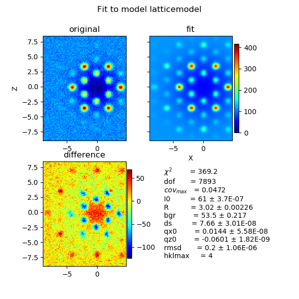
Fitting the 2D scattering of a lattice

This example shows how to fit a 2D scattering pattern as e.g. measured by small angle scattering.

As a first step one should fit radial averaged data to limit the lattice constants to reasonable ranges and deduce reasonable values for background and other parameters.

Because of the topology of the problem with a large plateau and small minima most fit algorithm (using a gradient) will fail. One has to take care that the first estimate of the starting parameters (see above) is already close to a very good guess or one may use a method to find a global minimum as differential_evolution or brute force scanning. This requires some time.

In the following we limit the model to a few parameters. One needs basically to include more as e.g. the orientation of the crystal in 3D and more parameters influencing the measurement. Prior knowledge about the experiment as e.g. a preferred orientation during a shear experiment is helpful information.

Another possibility is to normalize the data e.g. to peak maximum=1 with high q data also fixed.

As a good practice it is useful to first fit 1D data to fix some parameters and add e.g. orientation in a second step with 2D fitting.

import jscatter as js
import numpy as np

# load a image with hexagonal peaks (synthetic data)
image = js.sas.sasImage(js.examples.datapath + '/2Dhex.tiff')
image.setPlaneCenter([51, 51])
image.gaussianFilter()
# transform to dataarray with X,Z as wavevectors
# The fit algorithm works also with masked areas
hexa = image.asdataArray(0)


def latticemodel(qx, qz, R, ds, rmsd, hklmax, bgr, I0, qx0=0, qz0=0):
    # a hexagonal grid with background, domain size and Debye Waller-factor (rmsd)
    # 3D wavevector
    qxyz = np.c_[qx + qx0, qz - qz0, np.zeros_like(qx)]
    # define lattice
    grid = js.sf.hcpLattice(R, [3, 3, 3])
    # here one may rotate the crystal
    # calc scattering
    lattice = js.sf.orientedLatticeStructureFactor(qxyz, grid, domainsize=ds, rmsd=rmsd, hklmax=hklmax)
    # add I0 and background
    lattice.Y = I0 * lattice.Y + bgr
    return lattice


# Because of the high plateau in the chi2 landscape
# we first need to use a algorithm finding a global minimum
# this needs some time and maybe a good choice of starting parameters
if 0:
    # Please do this if you want to wait
    hexa.fit(latticemodel, {'R': 3, 'ds': 10, 'rmsd': 0.3, 'bgr': 16, 'I0': 90},
             {'hklmax': 5, }, {'qx': 'X', 'qz': 'Z'}, method='differential_evolution')
    #
    fig = js.mpl.surface(hexa.X, hexa.Z, hexa.Y, image.shape)
    fig = js.mpl.surface(hexa.lastfit.X, hexa.lastfit.Z, hexa.lastfit.Y, image.shape)

# We use as starting parameters the result of the previous fit
# Now we use LevenbergMarquardt algorithm to polish the result
hexa.fit(latticemodel, {'R': 3.02, 'ds': 8.3, 'rmsd': 0.27, 'bgr': 19, 'I0': 95, 'qx0': 0, 'qz0': 0},
         {'hklmax': 4, }, {'qx': 'X', 'qz': 'Z'}, diff_step=0.01)

fig = js.mpl.showlastErrPlot2D(hexa, shape=image.shape, transpose=1)

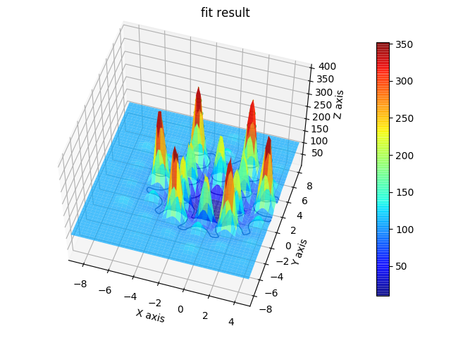
fig2 = js.mpl.surface(hexa.lastfit.X, hexa.lastfit.Z, hexa.lastfit.Y, image.shape)
fig2.suptitle('fit result')

Using cloudscattering as fit model

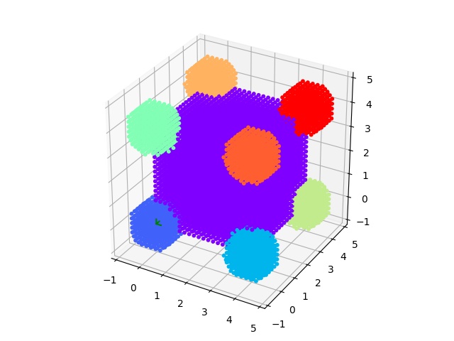
At the end a complex shaped object: A cube decorated with spheres of different scattering length.

# Using cloudScattering as fit model.
# We have to define a model that parametrize the building of the cloud that we get a fit parameter.
# As example we use two overlapping spheres. The model can be used to fit some data.

import jscatter as js
import numpy as np

#: test if distance from point on X axis
isInside = lambda x, A, R: ((x - np.r_[A, 0, 0]) ** 2).sum(axis=1) ** 0.5 < R


#: model
def dumbbell(q, A, R1, R2, b1, b2, bgr=0, dx=0.3, relError=100):
    # A sphere distance
    # R1, R2 radii
    # b1,b2  scattering length
    # bgr background
    # dx grid distance not a fit parameter!!
    mR = max(R1, R2)
    # xyz coordinates
    grid = np.mgrid[-A / 2 - mR:A / 2 + mR:dx, -mR:mR:dx, -mR:mR:dx].reshape(3, -1).T
    insidegrid = grid[isInside(grid, -A / 2., R1) | isInside(grid, A / 2., R2)]
    # add blength column
    insidegrid = np.c_[insidegrid, insidegrid[:, 0] * 0]
    # set the corresponding blength; the order is important as here b2 overwrites b1
    insidegrid[isInside(insidegrid[:, :3], -A / 2., R1), 3] = b1
    insidegrid[isInside(insidegrid[:, :3], A / 2., R2), 3] = b2
    # and maybe a mix ; this depends on your model
    insidegrid[isInside(insidegrid[:, :3], -A / 2., R1) & isInside(insidegrid[:, :3], A / 2., R2), 3] = (b2 + b1) / 2.
    # calc the scattering
    result = js.ff.cloudScattering(q, insidegrid, relError=relError)
    result.Y += bgr
    # add attributes for later usage
    result.A = A
    result.R1 = R1
    result.R2 = R2
    result.dx = dx
    result.bgr = bgr
    result.b1 = b1
    result.b2 = b2
    result.insidegrid = insidegrid
    return result


#
# test it
q = np.r_[0.01:10:0.02]
data = dumbbell(q, 4, 2, 2, 0.5, 1.5)
#
# Fit your data like this (I know that b1 abd b2 are wrong).
# It may be a good idea to use not the highest resolution in the beginning because of speed.
# If you have a good set of starting parameters you can decrease dx.
data2 = data.prune(number=200)
data2.makeErrPlot(yscale='l')
data2.setlimit(A=[0, None, 0])
data2.fit(model=dumbbell,
          freepar={'A': 3},
          fixpar={'R1': 2, 'R2': 2, 'dx': 0.3, 'b1': 0.5, 'b2': 1.5, 'bgr': 0},
          mapNames={'q': 'X'})

# An example to demonstrate how to build a complex shaped object with a simple cubic lattice
# Methods are defined in lattice objects.
# A cube with the corners decorated by spheres

import jscatter as js
import numpy as np

grid = js.sf.scLattice(0.2, 2 * 15, b=[0])
v1 = np.r_[4, 0, 0]
v2 = np.r_[0, 4, 0]
v3 = np.r_[0, 0, 4]
grid.inParallelepiped(v1, v2, v3, b=1)
grid.inSphere(1, center=[0, 0, 0], b=2)
grid.inSphere(1, center=v1, b=3)
grid.inSphere(1, center=v2, b=4)
grid.inSphere(1, center=v3, b=5)
grid.inSphere(1, center=v1 + v2, b=6)
grid.inSphere(1, center=v2 + v3, b=7)
grid.inSphere(1, center=v3 + v1, b=8)
grid.inSphere(1, center=v3 + v2 + v1, b=9)
fig = grid.show()
js.mpl.show()

Bayesian inference for fitting

method=’bayes’ uses Bayesian inference for modeling and the MCMC algorithms for sampling (we use emcee). Requires a larger amount of function evaluations but returns errors from Bayesian statistical analysis and allows inclusion of prior knowledge about parameters and restrictions.

For Bayesian analysis the log probability \(\ln\,p(y\,|\,x,\sigma,a) + ln(p(a_j))\) is maximized with the log likelihood \(ln (p(y\,|\,x,\sigma,a))\) and the prior \(p(a_j)\). Asuming Gaussian statistics we use

\[\ln\,p(y\,|\,x,\sigma,a) = -\frac{1}{2} \sum_i \left[\frac{(Y_i-f(X_i,a_1,..a_p))^2}{\sigma_i^2} + \ln \left ( p(a_j) \right )\right]\]

By default an uniform (so-called “uninformative”) prior is used

\[\begin{split}log(p(a_j)) = \left\{ \begin{array}{ll} 0 & \mbox{if $a_j$ in limits};\\ -inf & \mbox{otherwise}.\end{array} \right.\end{split}\]

which can be changed using the parameter ln_prior to be more informative. Assuming for parameter \(a_j\) a Gaussian distribution of deviations from a mean with width sigma

\[\ln \left ( p(a_j) \right ) = - \lambda \sum_i w_j^2\]

where for \(\lambda=0\) the prior vanishes.

\(\lambda\) quantifies of by how much we believe that e.g. \(w_j = a_j-a_{mean}\) should be close to zero and can be choosen as \(\lambda=n 0.5/\sigma^2\) assuming that \(a_j\) shoud be within a Gaussian of width sigma, maybe determined from a different measurement.

The scale \(n\) scales the Gaussian that the weight is comparable to the log likelihood. Using \(\lambda=0.5/\sigma^2\) weights the constrain equal to one datapoint.

In general the \(p(a_j)\) depend only on fit parameters \(a_j\) and not on \(Y_i\) or \(f(X_i,...)\). To allow more complex constraints, e.g. fitting a protein structure with the constrain that the backbone is not overstretched, the modelValues can be accessed if log_prior uses the keyword ‘modelValues’. Also the weigthed squared errors \(\chi^2_i=\frac{[Y_i-f(X_i,a_1,..a_p)]^2}{\sigma_i^2}\) can be accessed using the keyword ‘x2i’ to regularise in some way different meassurements according to their errors.

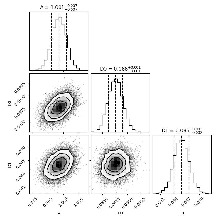
The example shows how some knowledge about parameters A and D that can be used for the prior. We assume here that the amplitude A is distributed around 1 within a Gaussian distribution and D around 0.09.

The evaluation might take somewhat longer for bayes (here 100s on my desktop).

import numpy as np
import jscatter as js
import matplotlib.pyplot as plt
import corner

# data to fit
# We use each a subset to speed up the example
i5 = js.dL(js.examples.datapath+'/iqt_1hho.dat')[[3, 5]]

# model
def diffusion(A, D, t, elastic, wavevector=0):
    return A*np.exp(-wavevector**2*D*t) + elastic

# Define ln_prior that describes knowledge about the data, parameters or how parameters are distributed.
# The ln_prior is complemented by the limits as:
# 0 within limits (log(1)) and -inf outside limits (log(0))
# Without prior only the limits are used (uninformative prior) that
# the prior is optional if you know something about the parameters.

# As the prior is a probability it should be normalized. On the other side, as in the examples,
# the normalisation constants result in constant offset dependent on sigma
# and will not influence the best fit result but chi2.

# To be compatible with regularisation the ln_prior is written here as positive and
# internally  multiplied by `-1`.

Amean, Asig = 1.0 , 0.01
Dmean, Dsig = 0.09 , 0.02
def ln_priorGAUSS(A, D):
    # assuming a normalized Gaussian distribution around the mean of A and D with width sig (Gaussian prior)
    # https://en.wikipedia.org/wiki/Normal_distribution
    # the log of the Gaussian is the log_prior, the second log is from the Gaussian normalisation
    # negative sign like common literature
    # the parameters are arrays for all elements of the dataList or a float for common parameters
    # the 't' is not included as it describes the .X values, 'elastic' is not used (no knowledge about it).
    lp = -0.5 * np.sum((A-Amean)**2/Asig**2) - (0.5 * np.log(2*np.pi) + np.log(Asig)) * len(A)
    lp += -0.5 * np.sum((D-Dmean)**2/Dsig**2) - (0.5 * np.log(2*np.pi) + np.log(Dsig)) * len(D)
    # return negative to be regularisation compatible
    return -lp

# as example => Laplace prior.
# The Laplace prior has fatter tails than the Gaussian, and is also more concentrated around zero.
def ln_priorLAPLACE(A, D):
    # while Gauss uses L2 norm , here we use L1 norm =>|A-Amean|
    # https://en.wikipedia.org/wiki/Laplace_distribution
    lp = -  np.sum(np.abs(A-Amean)/(2**0.5*Asig)) + np.log(1/(2*2**0.5*Asig)*len(A))
    lp += - np.sum(np.abs(D-Dmean)/2**0.5*Dsig) + np.log(1/(2*2**0.5*Dsig)*len(D))
    # return negative to be regularisation compatible
    return -lp

i5.setlimit(D=[0.05, 1], A=[0.5, 1.5])

# do Bayesian analysis with the prior
i5.fit(model=diffusion, freepar={'D': [0.2], 'A': 0.98}, fixpar={'elastic': 0.0},
      mapNames={'t': 'X', 'wavevector': 'q'}, condition=lambda a: a.X<90,
       method='bayes', tolerance=20, bayesnsteps=1000, ln_prior=ln_priorGAUSS)

i5.showlastErrPlot()

# get sampler chain and examine results removing burn in time 2*tau
tau = i5.getBayesSampler().get_autocorr_time(tol=20)
flat_samples = i5.getBayesSampler().get_chain(discard=int(2*tau.max()), thin=1, flat=True)
labels = i5.getBayesSampler().parlabels

plt.ion()
fig = corner.corner(flat_samples, labels=labels, quantiles=[0.16, 0.5, 0.84], show_titles=True, title_fmt='.3f')
plt.show()
# fig.savefig(js.examples.imagepath+'/bayescorner_withprior.jpg')

If we neglect the normalisation terms -ln_prior is the regularisation term used below.

Regularisation for fitting

Regularisation in least squares offers the posibility to use prior knowledge similar to ‘bayes’ to constrain the solution. Different to ‘bayes’ it uses the faster \(\chi^2 minimization\) algorithms with the additional constrain \(\propto ln(p(w))\). For a Gaussian prior \(p(w)\) corresponds to ridge regression and for a Laplace prior to Lasso regression . You can define whatever you want (some things are more justified than others) as long as there is a minimum and \(ln(p(w))>0\).

For \(\chi^2 minimization\) we minimise \(\chi_{red}^2 - ln(p(a_j))\). For a Gaussian prior (Ridge regression) this is

\[\chi^2 = \frac{1}{n-p} \sum_i^n \frac{[Y_i-f(X_i,a_1,..a_p)]^2}{\sigma_i^2} + \lambda \sum_j w_j^2\]

where for \(\lambda=0\) the conventional \(\chi_{red}^2 minimization\) is retrieved.

\(\lambda\) quantifies of by how much we believe that e.g. \(w_i = A-A_{mean}\) should be close to zero and can be choosen as \(\lambda=\frac{1}{n}0.5/\sigma^2\) similar to the above ln_prior assuming that A shoud be within a Gaussian of width sigma, maybe determined from a different measurement.

Selects the weight you want to apply :

• Using \(\lambda=0.5/\sigma^2\) for a single variable in Gaussian distribution would be weighted like all measurement values in \(\chi_{red}^2\) together.

• A divisor 1/n scales the Gaussian that the weight is comparable to one data point.

• Weighing with \(1/n_{j}\) weight each \(w_j\) like \(\chi_{red}^2\).

• If the \(\lambda \sum_j w_j^2\) are to strong weigthed, this will dominate the result.

• For the below example with i5 containing 16 Q values with about 20 points a weight equal to 20 points corresponding to one Q might be reasonable.

In general the \(p(a_j)\) depend only on fit parameters \(a_j\) and not on \(Y_i\) or \(f(X_i,...)\). The best \(\lambda\) may be selected from a series of tries as the one with best fit results.

To allow more complex constraints the modelValues can be accessed if log_prior uses the keyword modelValues. The weigthed squared errors \(\chi^2_i=\frac{[Y_i-f(X_i,a_1,..a_p)]^2}{\sigma_i^2}\) can be accessed as modelValues.chi2i and degrees of freedom as modelValues.dof. Anything calculated in the model can be accessed in modelValues.

This can be used to constrain by something calculated in the model or to weight e.g. different meassurements according to their errors, number of datapoints or relative contribution to \(\chi^2\).

The example shows how some knowledge about parameters A and D can be used for the regularisation. We assume here that the amplitude A is distributed around 1 within a Gaussian distribution and D around 0.09.

!!! The example is an example for to strong constraints. Its more how to do it and here without advantage.

import numpy as np
import jscatter as js

# data to fit
# We can fit all as it is faster than bayes
i5 = js.dL(js.examples.datapath+'/iqt_1hho.dat')

# model
def diffusion(A, D, t, elastic, wavevector=0):
    return A*np.exp(-wavevector**2*D*t) + elastic

# Define regularization function that describes knowledge about the data, parameters or how parameters are distributed.
Amean, Asig = 1.0 , 0.01
Dmean, Dsig = 0.09 , 0.02
def ln_priorGAUSS(A, D):
    # assuming a normalized Gaussian distribution around the mean of A and D with width sig (Gaussian prior)
    # the log of the Gaussian is ~ lambda*w**2 = 0.5/Asig**2 * (a-Amean)**2,
    # lambda*w**2 should be always positive without normalisation.
    # the parameters are arrays for all elements of the dataList or a float for common parameters
    # the 't' is not included as it describes the .X values, 'elastic' is not used (no knowledge about it).
    lp = 0.5 * np.sum((A-Amean)**2/Asig**2)
    lp += 0.5 * np.sum((D-Dmean)**2/Dsig**2)
    return lp

# as example => Laplace prior.
# The Laplace prior has fatter tails than the Gaussian, and is also more concentrated around zero.
def ln_priorLAPLACE(A, D):
    # while Gauss uses L2 norm , here we use L1 norm =>|A-Amean|
    lp =  np.sum(np.abs(A-Amean)/(2**0.5*Asig))
    lp += np.sum(np.abs(D-Dmean)/2**0.5*Dsig)
    return lp

# as example => Gaussian around the average only for A and usage of current modelValues.
# if ln_prior has keyword 'modelValues' these are added from the current calculation
def ln_priorMEAN(modelValues, A):
    # for a free A we want that these are within some sigma with unknown mean.
    lp =  np.sum(np.abs(A-np.mean(A))**2) / Asig**2
    # this is a stupid example as demonstration
    # e.g. in SAXS it might be I0 or Rg that determine a penalty
    # that is not in the parameters but in the formfactor calculation
    lp += 0 if modelValues.Y[:5,0].mean > 0.9 else 10

    return lp


i5.setlimit(D=[0.05, 1], A=[0.5, 1.5])

# do the fit with regression constrain in  ''ln_prior''.
i5.fit(model=diffusion, freepar={'D': [0.2], 'A': 0.98}, fixpar={'elastic': 0.0},
      mapNames={'t': 'X', 'wavevector': 'q'}, condition=lambda a: a.X<90,
      method='lm', ln_prior=ln_priorGAUSS)

i5.showlastErrPlot()

p=js.grace()
p.plot(i5.q,i5.D,i5.D_err,le='Too strong regularization')

# The result is not good as the constraint on D is too much constraining the diffusion coefficient.
# Therefore, the errors are large and the values to close to 0.09.
# better is simple 'lm' without constrain in this case.
# This was wrong knowledge assuming D is constant!

i5.fit(model=diffusion, freepar={'D': [0.2], 'A': 0.98}, fixpar={'elastic': 0.0},
       mapNames={'t': 'X', 'wavevector': 'q'}, condition=lambda a: a.X<90,
       method='lm',output=False)
p.plot(i5.q,i5.D,i5.D_err,le='LevenbergMarquardt fit')
p.legend(x=0.1,y=0.13)
p.yaxis(min=0.05,max=0.15)

Iterative reweighting of multiple measurements

In a combined fit of \(K\) datasets of different types, a naive summation of \(\chi^2\) contributions - assuming identical and independent distribution of deviations - causes large datasets or dataset with systematically smaller error to dominate the minimization. Reweighting corrects this by assigning each dataset a weight \(w_k\) like \(\chi^2= \sum_k w_k\chi^2_k\).

Application : As an example we might think about a NSE measurement with good defined error bars and a dynamic light scattering (DLS) measurement which typically gives no error at all for the correlation function. Here we can estimate an error for DLS and refine this estimate. Another application might be to identify dataset that need larger reweighting because of suspicious data or error estimates, e.g a large number of zero counts in bins or wrong counting during the measurement, and identify outliers.

Using different weights was introduced by [1] and others as Iteratively Reweighted Least-Squares (IRLS). IRLS iteratively calculates weights of individual data points and simultaneously tries to find model parameters that fit the bulk of the data using a least-squares approach, to produce estimates robust against outliers. Reweighting of datasets from different measurements was used by Larsen and Pedersen for combined fit of SAXS and SANS measyrements [2], [3].

Here we describe a iterative Expectation-Maximization (EM) algorithm used with the command regularizedEM() as an iterative reweighting of different mesurements like SAXS/SANS with different contrast or combining masurements of different instruments like neutron time of flight, backscattering and neutron spin echo as combined in [4] or [5]. Iterative reweigthing avoids time consuming Bayesian inference by faster iteration using standard fit routines. This is in particular useful if the model evaluation takes some time.

Excurs: Bayesian Analysis with precision hyperparameter

Bayesian Analysis

In the Bayesian framework the combined fit is formulated as a posterior distribution over the model parameters \(\theta\) and per-dataset precision hyperparameters \(\alpha_k\):

\[P(\theta, \{\alpha_k\} \mid \mathrm{data}) \propto P(\theta) \prod_{k=1}^{K} \mathcal{L}_k(\theta, \alpha_k)\, P(\alpha_k),\]

where the Gaussian likelihood for dataset \(k\) is

\[\ln \mathcal{L}_k(\theta, \alpha_k) = \frac{N_k}{2}\ln\alpha_k - \frac{\alpha_k}{2}\,\chi^2_k(\theta),\]

and \(\alpha_k\) rescales the trustworthiness of dataset \(k\) — large \(\alpha_k\) means the dataset is weighted heavily, small \(\alpha_k\) means it is down-weighted. Without rescaling the likelihood is only \(\ln \mathcal{L}_k(\theta)=-\frac{1}{2}\chi^2_k(\theta)\).

The conjugate prior for \(\alpha_k\) - our prior knowledge - is the Gamma distribution

\[P(\alpha_k) = \mathrm{Gamma}(\alpha_k \mid a_k, b_k) \propto \alpha_k^{a_k-1}\,e^{-b_k \alpha_k},\]

whose kernel matches the likelihood in \(\alpha_k\) exactly, so the posterior on \(\alpha_k\) is also Gamma with updated parameters:

\[P(\alpha_k \mid \theta, \mathrm{data}) = \mathrm{Gamma}\!\left(a_k + \tfrac{N_k}{2},\; b_k + \tfrac{\chi^2_k(\theta)}{2}\right),\]

with posterior mean

\[\langle\alpha_k\rangle = \frac{a_k + N_k/2}{b_k + \chi^2_k(\theta)/2}.\]

Marginalizing \(\alpha_k\) out of the joint posterior yields a marginal posterior over \(\theta\) alone, in which the uncertainty of each dataset’s error calibration is propagated into the parameter estimates rather than ignored.

The prior parameters \(a_k\) and \(b_k\) control the degree of regularisation:

• \(a_k = b_k = 0\) (Jeffreys): no prior knowledge; weights adapt freely to the data.

• \(a_k = b_k = 2\) (weakly informative): prior mean \(\langle\alpha_k\rangle_0 = 1\), expressing the belief that stated errors are approximately correct while allowing adaptation.

• \(a_k = b_k = N_k/2\) (strongly informative): prior mean 1 with variance \(\propto 1/N_k\), strongly constraining \(\alpha_k \approx 1\).

The EM-algorithm applied to a Bayesian model in which each dataset carries a precision hyperparameter \(\alpha_k \sim \mathrm{Gamma}(a_k, b_k)\) is an iterative procedure with an Expectation and a Maximization step. The general weight update at each iteration \(\nu\) using the posterior mean is

\[w_k^{(\nu+1)} = \langle\alpha_k\rangle = \frac{a_k + N_k/2}{b_k + {\chi^2_k}^{(\nu)}/2} = \frac{N_k + 2a_k}{{\chi^2_k}^{(\nu)} + 2b_k},\]

where \(N_k^{\mathrm{eff}} = N_k + 2a_k\) is an effective sample size inflated by the prior, and \(\chi^2_{\mathrm{reg},k} = 2b_k\) is a regularisation floor that prevents \(w_k\) from diverging when \({\chi^2_k}^{(\nu)} \to 0\). Convergence is guaranteed because each EM iteration increases the marginal posterior \(P(\theta \mid \mathrm{data})\).

The iterative reweighting algorithm is the EM-algorithm applied to this model: the E-step replaces \(\alpha_k\) by its posterior mean \(\langle\alpha_k\rangle\) given the current parameters, and the M-step maximises the resulting weighted cost over \(\theta\). This is equivalent to empirical Bayes — the hyperparameters \(\alpha_k\) are estimated from the data itself rather than fixed in advance.

The regularized EM-algorithm uses for \(\chi^2 minimization\) the total cost function \(C(\theta)\) (with parameters \(\theta = X_i,a_1,..a_p\))

\[C(\theta) = \frac{1}{K} \sum_{k=1}^{K} w_k \, \chi^2_{\mathrm{red},k} , \qquad \chi^2_{\mathrm{red},k} = \frac{\chi^2_k(\theta)} {N_k}, \qquad \chi^2_k(\theta) = \sum_{i \in k} \frac{\bigl(Y_i - f_i(\theta)\bigr)^2}{\sigma_i^2},\]

where \(N_k\) is the number of datapoints in dataset \(k\). The total cost function is defined as the mean of per-dataset reduced \(\chi^2\) values, normalised so that a good combined fit gives \(C \approx 1\), directly analogous to the single-dataset criterion \(\chi^2_{\mathrm{red}} \approx 1\):

The iteration is initialised at the prior mean \(w_k^{(0)} = a_k/b_k\). For the Jeffreys prior the prior mean is undefined and \(w_k^{(0)} = 1\) is used as a neutral starting point. An initial M-step with these weights produces the first residuals \({\chi^2_k}^{(0)}\) from which the E-step computes the first data-informed weights.

At convergence, the fixed point condition

\[w_k^{(\infty)} \cdot {\chi^2_{\mathrm{red},k}}^{(\infty)} = 1 \qquad \forall\, k\]

holds for every dataset individually, and the total cost satisfies \(\langle C \rangle = 1\).

The reweighting implies that \(\chi^2_{red} \to 1\) that it is not anymore a measure of fit quality but individual unweighted \(\chi^2_{\mathrm{red},k}\) still describe the fit quality for each dataset and can be used to determine a better error estimate (DLS above) or to identify suspicious data with high reweighting.

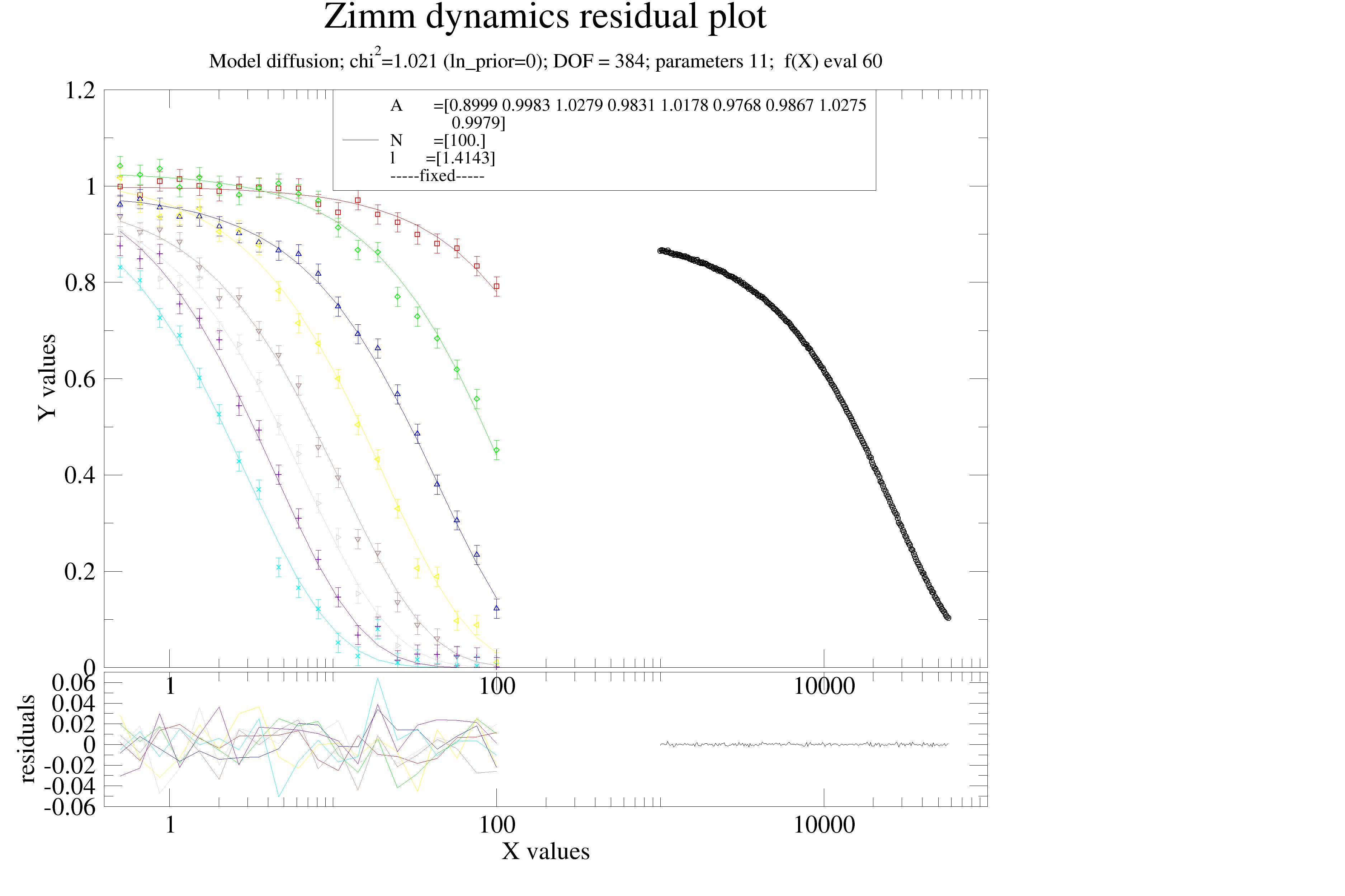
A short example: Zimm dynamics of a polymer in theta-solvent with DLS and NSE. Iterative reweighting is used to detect the wrong errors in synthetic data.

import jscatter as js
import numpy as np

def diffusion(A, t, q, N=200, l=1):
    zimm = js.dynamic.finiteZimm(t, q, N, 30, l=l, Dcm=None, tintern=0., Temp=273 + 20)
    #HP = js.dynamic.diffusionHarmonicPotential(t,q,rmsd,tau)
    zimm.Y = A * zimm.Y
    return zimm

# generate data with known properties
data = js.dL()
# typical DLS data: lambda 633 nm theta=173 degrees intercept 0.8 and cut at Y<0.1 and error 0.001
qq = 0.026
t = js.loglist(1e3,1e6,400)
diff = diffusion(0.9, t, qq)
dls = js.dA(np.c_[t, diff.Y + 0.001*np.random.randn(len(t)), t * 0 + 0.005].T)   # => errors too large
dls = dls[:,dls.Y>0.1]  # cut long times as usually done for  DLS
data.append(dls)
data[-1].q = qq
data[-1].type='dls'

# NSE data with 20 timevalues
ef = 0.02
t = js.loglist(0.5,100,20)
A = np.random.normal(1,0.02,8)
for qq,a in zip(np.r_[0.2:1.8:12j],A):
    diff = diffusion(a, t, qq)
    data.append(js.dA(np.c_[t, diff.Y + ef*np.random.randn(len(t)), t * 0 + ef].T))
    data[-1].q = qq
    data[-1].type='nse'
# ----------------------------------


# standard fit as start
data.makeErrPlot(title='Zimm dynamics residual plot', xscale='log',legpos=[0.2, 0.8])
data.fit(model=diffusion,
   freepar={'A':[1], 'N':100, 'l':2 }, fixpar={},
   mapNames={'t': 'X'},)
data.errplot[0].yaxis(min=0,max=1.2)
data.errplot[0].legend(x=10,y=1.2)
# data.savelastErrPlot(js.examples.imagepath+'/iterativeReweight.jpg',size=(2,2),dpi=200)

# check chi^2_{red,k} for each dataset
data.reducedChi2k()  # DLS chi2_k is quite small fit not bad here

# regularisation steps 3 for dataArrays
weights, convergence = data.regularizedEM(a=1,b=1, steps=3)
# weights => dls weight ~20 times smaller
# convergence bad => a=1,b=1 too strong (because of DLS)

# repeat with a=0, b=0
weights, convergence = data.regularizedEM(a=0,b=0, steps=3)
# weight ~23 as dls error is 5 times to large ~5**2=25
#
# check chi^2_{red,k} for each dataset
data.reducedChi2k()  # DLS chi2_k is quite small fit not bad here

# regularisation steps 3 for dataArrays
# here only differentiating for measurement type as ['dls',  'nse']
weights, convergence = data.regularizedEM(a=[0,'type'],b=[0], steps=3)

• Regularisation with a non-informative prior

  With a Jeffreys prior (non-informative prior) using \(\mathrm{Gamma}(a_k \to 0, b_k \to 0)\), the posterior mean of \(\alpha_k\) at fixed \(\theta\) is

  \[\langle\alpha_k\rangle = \frac{a_k + N_k/2}{b_k + \chi^2_k/2} \xrightarrow{\,a_k,\,b_k\,\to\,0\,} \frac{N_k}{\chi^2_k} = \frac{1}{\chi^2_{\mathrm{red},k}},\]

  The weights are updated at each iteration \(\nu\) as \(w_k^{(\nu+1)} = 1 / {\chi^2_{\mathrm{red},k}}^{(\nu)}\). The initial weights \(w_k^{(0)} = 1\) correspond to equal weighting of all datasets in reduced \(\chi^2\) units, which is the prior expectation that all datasets are correctly normalised.

  The Jeffreys case adds no information beyond what the data contain. So in the strict sense the Jeffreys EM iteration is not regularisation.

• Regularisation with an informative prior

  The iterative reweighting scheme can be stabilised by replacing the Jeffreys prior on \(\alpha_k\) with an informative \(\mathrm{Gamma}(a_k >0, b_k>0)\) prior. This is particularly useful for small datasets where \(\chi^2_{\mathrm{red},k}\) is noisy and the unregularised weights may fluctuate strongly between iterations.

Three natural choices of prior are summarised below. Remember that for \(\mathrm{Gamma}(a_k, b_k)\) the \(mean=a/b\) and \(\sigma^2=a/b^2\) .

Prior	\(a_k\)	\(b_k\)	Effect
Jeffreys (no regularisation)	\(0\)	\(0\)	Weights vary freely; exact recovery of \(N_k/\chi^2_k\); can be noisy for small \(N_k\)
Weakly informative	\(2\)	\(2\)	\(\mu=1\); \(\sigma^2=1/2\); floor \(2b_k=4\); update \((N_k+4)/(\chi^2_k+4)\)
Strongly informative	\(N_k/2\)	\(N_k/2\)	\(\mu=1\); \(\sigma^2 \propto 1/N_k\); enforces \(\chi^2_{\mathrm{red},k}\approx 1\) as hard constraint

The weakly informative choice \(a_k = b_k = 2\) is recommended as a default. It centres \(\alpha_k\) near 1, expressing the belief that the stated errors are approximately correct, while still allowing the weights to adapt if a dataset is systematically over- or under-weighted. The resulting update

\[w_k^{(\nu+1)} = \frac{N_k + 4}{{\chi^2_k}^{(\nu)} + 4}\]

differs negligibly from the Jeffreys rule for large \(N_k\), but suppresses erratic weight changes when \(N_k\) is small. The convergence criterion

\[w_k^{(\infty)} \cdot {\chi^2_{\mathrm{red},k}}^{(\infty)} \approx 1 \qquad \forall\, k\]

still holds to within corrections of order \(2 a_k/N_k\), which vanish as \(N_k \to \infty\).

Note

For the strongly informative prior \(a_k = b_k = N_k/2\), the weight update is

\[w_k^{(\nu+1)} = \frac{2N_k}{{\chi^2_k}^{(\nu)} + N_k},\]

and the convergence criterion evaluates to

\[w_k^{(\infty)} \cdot {\chi^2_{\mathrm{red},k}}^{(\infty)} = \frac{2{\chi^2_{\mathrm{red},k}}^{(\infty)}} {1 + {\chi^2_{\mathrm{red},k}}^{(\infty)}},\]

which equals 1 only when \({\chi^2_{\mathrm{red},k}}^{(\infty)} = 1\), confirming that this prior enforces correct error calibration as a hard constraint.

Warning

If a dataset shows \(\chi^2_{\mathrm{red},k} \gg 1\) at convergence even with the strongly informative prior, this indicates model inadequacy rather than error misestimation. Per-dataset residuals should always be inspected after convergence.

References

[1]

Robust Regression Using Iteratively Reweighted Least-Squares. Holland, P. W.; Welsch, R. E. Communications in Statistics - Theory and Methods 1977, 6 (9), 813–827. https://doi.org/10.1080/03610927708827533.

[2]

Optimal Weights and Priors in Simultaneous Fitting of Multiple Small-Angle Scattering Datasets. Larsen, A. H. J Appl Cryst 2025, 58 (3), 934–947. https://doi.org/10.1107/S1600576725002390.

[3]

Experimental Noise in Small-Angle Scattering Can Be Assessed Using the Bayesian Indirect Fourier Transformation. Larsen, A. H.; Pedersen, M. C. Journal of Applied Crystallography 2021, 54 (5), 1281–1289. https://doi.org/10.1107/S1600576721006877.

[4]

Dynamic fluctuations in a highly cross-linked polybutadiene rubber Rosi et al J. Chem. Phys. 162, 214902 (2025) https://doi.org/10.1063/5.0265589

[5]

Fast internal dynamics in alcohol dehydrogenase. Monkenbusch, M., Stadler, A., Biehl, R., Ollivier, J., Zamponi, M. & Richter, D. Journal of Chemical Physics, 143, 075101 (2015), https://doi.org/10.1063/1.4928512