Build models

How to build simple models

# How to build simple models
# which are actually not so simple....

import numpy as np
import jscatter as js

# Build models in one line using lambda
# directly calc the values and return only Y values
diffusion = lambda A, D, t, wavevector, elastic=0: A * np.exp(-wavevector ** 2 * D * t) + elastic

# use a model from the libraries
# here Teubner-Strey adding background and power law
# this returns as above only Y values
tbpower = lambda q, B, xi, dd, A, beta, bgr: js.ff.teubnerStrey(q=q, xi=xi, d=dd).Y * B + A * q ** beta + bgr


# The same as above in a function definition
# This should be the preferred way
def diffusion2(A, D, t, elastic, wavevector=0):
    Y = A * np.exp(-wavevector ** 2 * D * t) + elastic
    return Y


# returning dataArray allows additional attributes to be included in the result
# this returns a dataArray with X, Y values and attributes
# and is how Jscatter model return data
def diffusion3(A, D, t, wavevector, elastic=0):
    Y = A * np.exp(-wavevector ** 2 * D * t) + elastic
    result = js.dA(np.c_[t, Y].T)
    result.diffusioncoefficient = D
    result.wavevector = wavevector
    result.columnname = 'time;Iqt'
    return result


# supplement an existing model
def tbpower2(q, B, xi, dd, A, beta, bgr):
    """Model Teubner Strey  + power law and background"""
    # save different contributions for later analysis
    tb = js.ff.teubnerStrey(q=q, xi=xi, d=dd)
    pl = A * q ** beta  # power law
    tb = tb.addZeroColumns(2)
    tb[-2] = pl  # save power law in new last column
    tb[-1] = tb.Y  # save Teubner-Strey in last column
    tb.Y = B * tb.Y + pl + bgr  # put full model to Y values (usually tb[1])
    # save the additional parameters ; xi and d already included in teubnerStrey
    tb.A = A
    tb.bgr = bgr
    tb.beta = beta
    tb.columnname = 'q;Iq,IqTb,Iqpower'
    return tb

# How to add a numpy like docstring see in the example "How to build a complex model".

How to build a more complex model

# How to build a complex model

import jscatter as js

resol2m = js.sas.prepareBeamProfile('SANS', detDist=2000, collDist=2000., wavelength=0.7, wavespread=0.10,
                                    collAperture=30, sampleAperture=6, dpixelWidth=10, dringwidth=1)


# build a complex model of different components inclusive smearing
# @js.sas.smear does the smearing of the model in the following line

@js.sas.smear(beamProfile=resol2m)
def particlesWithInteraction(q, Ra, Rb, molarity, bgr, contrast=1, detDist=None, collDist=None, beta=True):
    """
    Particles with interaction and ellipsoid form factor as a model for e.g. dense protein solutions.

    Document your model if needed for later use that you know what you did and why.
    Or make it short without all the nasty documentation for testing.
    The example neglects the protein exact shape and non constant scattering length density.
    Proteins are more potato shaped  and nearly never like a ellipsoid or sphere.
    So this model is only valid at low Q as an approximation.

    Parameters
    ----------
    q : float
        Wavevector
    Ra,Rb : float
        Radius
    molarity : float
        Concentration in mol/l
    contrast : float
        Contrast between ellipsoid and solvent.
    bgr : float
        Background e.g. incoherent scattering
    detDist,collDist : float, None
        detector distance and collimation length for SANS and SAXS.
        If any is None no smearing is used.
        Both need not to be used in the model function.
    beta : bool
        True include asymmetry factor beta of
        M. Kotlarchyk and S.-H. Chen, J. Chem. Phys. 79, 2461 (1983).

    Returns
    -------
        dataArray

    Notes
    -----
    Explicitly:
    **The return value can be a dataArray OR only Y values**. Both is working for fitting.

    **About smearing during a fit with mixed SANS and or SAXS**:

    Data to fit should have attributes with smear parameters as detDist and more .
    For SAXS we set detDist=None (bypass smearing ==no smearing) or we set parameters for SAXS smearing.
    For SANS  we set some reasonable values as 2000 (mm) or 20000 (mm) for detDist and collDist.
    Missing parameters are used from beamProfile as given in the decorator.

    """
    # We need to multiply form factor and structure factor and add an additional background.
    # formfactor of ellipsoid returns dataArray with beta at last column.
    ff = js.ff.ellipsoid(q, Ra, Rb, SLD=contrast)
    V = ff.EllipsoidVolume
    # the structure factor returns also dataArray
    # we need to supply a radius calculated from Ra Rb, this is an assumption of effective radius for the interaction.
    R = (Ra * Rb * Rb) ** (1 / 3.)
    # the volume fraction is concentration * volume
    # the units have to be converted as V is usually nm**3 and concentration is mol/l
    sf = js.sf.PercusYevick(q, R, molarity=molarity)
    if beta:
        # beta is asymmetry factor according to M. Kotlarchyk and S.-H. Chen, J. Chem. Phys. 79, 2461 (1983).
        # correction to apply for the structure factor
        # noinspection PyProtectedMember
        sf.Y = 1 + ff._beta * (sf.Y - 1)
    #
    # molarity (mol/l) with conversion to number/nm**3 result is in cm**-1
    ff.Y = molarity * 6.023e23 / (1000 * 1e7 ** 2) * ff.Y * sf.Y + bgr
    # add parameters for later use; ellipsoid parameters are already included in ff
    # if data are saved these are included in the file as documentation
    # or can be used for further calculations e.g. if volume fraction is needed (V*molarity)
    ff.R = R
    ff.bgr = bgr
    ff.Volume = V
    ff.molarity = molarity

    return ff


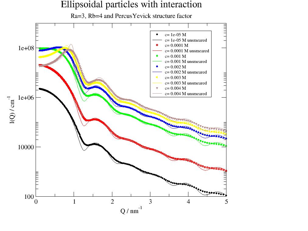
p = js.grace()
q = js.loglist(0.1, 5, 300)
for i, m in enumerate([0.01, 0.1, 1, 2, 3, 4], 1):
    data = particlesWithInteraction(q, Ra=3, Rb=4, molarity=m * 1e-3, bgr=0, contrast=1, detDist=2000, collDist=2000)
    p.plot(data, sy=[i, 0.3, i], le='c= $molarity M')
    p.plot(data.X, data[2], sy=0, li=[1, 1, i], le='c= {0:} M unsmeared'.format(data.molarity))

p.legend(x=3, y=5e8, charsize=0.7)
p.yaxis(min=100, max=1e9, scale='l', label=r'I(Q) / cm\S-1', tick=[10, 9])
p.xaxis(scale='n', label=r'Q / nm\S-1')
p.title('Ellipsoidal particles with interaction')
p.subtitle('Ra=3, Rb=4 and PercusYevick structure factor')
# Hint for fitting SANS data or other parameter dependent fit:
# For a combined fit of several collimation distances each dataset should contain an attribute data.collimation.
# This is automatically used in the fit, if there is not explicit fit parameter with this name.

if 1:
    p.save('interactingParticles.agr')
    p.save('interactingParticles.jpeg')