Dynamic models
This shows dynamic models and how to fit inelastic neutron scattering data from backscattering or time of flight experiments. The classical models are in the module dynamic and can be combined similar to the first example. The actual way how data are combined depends on the idea which atoms contribute to which process. This is more visible in later examples.
One example shows how to fit different instruments together.
Some dynamic models related to bio are shown in Biomacromolecules (bio).
Multi component models for data inspection at inelastic instruments
Here we use a simple two Lorentz model for data inspection or as general receip. The model can be adopted to the needs of the experiment mixing different models e.g translational diffusion and sidechains diffusion in a harmonic potential.
A more complex model that includes that all atoms contribute to COM diffusion and only a part to faster movements is shown later.
As resolution we use normalized experimental data to make it simple and stay close to the experiment.
As simple yet powerful predefined models doubleStretchedExp_w()
and threeLorentz_w() can be used in the same way.
Many published papers dont go beyond these simple models.
The data in the example were measured by Margarita Kruteva and Benedetta Rosi at EMU@ANSTO and the empty cell measurement is already subtracted in Mantid.
import jscatter as js
import numpy as np
from jscatter.dynamic import convolve
from jscatter.dynamic import lorentz_w
js.usempl(True)
def readinx(filename, block, l2p, instrument):
# reusable function for inx reading
# neutron scatterers use strange data formats like .inx dependent on instrument and local contact
# blocks start with number of channels. Spaces around the number (' 562 ') are important to find the starting line.
# this might dependent on instrument
data = js.dL(filename,
block=block, # this finds the starting of the blocks of all angles or Q
usecols=[1, 2, 3], # ignore the numbering at each line
lines2parameter=l2p) # catch the parameters at beginning
for da in data:
da.channels = da.line_1[0]
da.Q = da.line_3[0] # in 1/A # it might be necessary to calc the Q here
da.incident_energy = da.line_3[1] # in meV
da.temperature = da.line_3[3] # in K if given
da.instrument = instrument
return data
# data exported from Mantid look different, simpler. These have only the parameter Q in front of a block
# these can be read like this e.g. from EMU exported by Mantid
def readEMUdat(filename, wavelength=6.27084, temperature=0):
"""
Read data form EMU@ANSTO as direct output from Mantid (No .inx conversion needed)
"""
data = js.dL(filename, delimiter=',')
for da in data:
da.Q = np.round(float(da.comment[0]), 4)
da.temperature = temperature
da.wavelength = wavelength
# cut the zero at the end
for i in range(len(data)):
data[i] = data[i, :, :-1]
return data
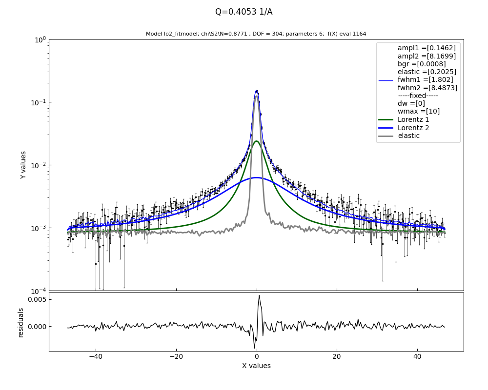
def lo2_fitmodel(w, dw, Q, amp1, amp2, fwhm1, fwhm2, elastic, bgr, resolution, wmax=None):
"""
Model : elastic with two Lorentz functions and using experimental data for resolution convolution.
w : frequencies 1/ns
dw : center shift
amp, amp2 : Lorentz amplitudes
fwhw1,fwhw2 : full width half maximum pf Lorentz
elastic : amplitude elastic contribution
bgr : const background
resolution : datalist with measured resolution and parameters Q same as in fit data
wmax : cutoff frequency for resolution
"""
if wmax is None:
wmax = max(np.abs(w))
# get right Q value of resolution for selected vana and prune to max frequency
resolutionQ = resolution.filter(Q=Q)[0]
# two Lorentz model and elastic , all same w
model1 = lorentz_w(w, fwhm1)
model1.Y = amp1 * model1.Y
# model2 = transDiff_w(w, q=Q, D=Dt) # alternative model; parameters need to be adopted
model2 = lorentz_w(w, fwhm2)
model2.Y = amp1 * model2.Y
# sum amplitudes and put in copied lorentz1
both = model1.copy()
both.Y = model1.Y + model2.Y
# convolve with resolution; convolve also intermediate steps to use in later plots
convboth = convolve(both, resolutionQ.prune(-wmax, wmax, weight=None), normB=True).interpolate(w)
convmodel1 = convolve(model1, resolutionQ.prune(-wmax, wmax, weight=None), normB=True).interpolate(w)
convmodel2 = convolve(model2, resolutionQ.prune(-wmax, wmax, weight=None), normB=True).interpolate(w)
# compose the data to return
# use resolution as elastic contribution
result = js.dA(np.c_[w, # frequencies
convboth.Y + elastic * resolutionQ.Y + bgr, # fit model
convmodel1.Y + bgr, # component 1
convmodel2.Y + bgr, # component 2
elastic*resolutionQ.Y+bgr].T) # elastic contribution
# append some of the intermediate contributions and add columnames to access components later
result.columnname = 'w;both;m1;m2;el'
result.elastic = elastic
result.fwhm1 = fwhm1
result.fwhm2 = fwhm2
result.amp1 = amp1
result.amp2 = amp2
return result
# load experimental resolution and convert to 1/ns
# For emu the block is ' 314 ' with 2 spaces in front of the number and 1 after
# resolution experimental data
vanae = readEMUdat(js.examples.datapath + '/sample_5K_Q.dat.gz', temperature=5)
vana = js.dynamic.convert_e2w(vanae, 0, unit='meV')
# convert resolution to normalized data that elastic has meaning
for va in vana:
va.Y = va.Y/np.trapezoid(va.Y,va.X)
# read new data and convert to 1/ns
same = readEMUdat(js.examples.datapath + '/sample_413K_Q.dat.gz',temperature=413)
sam = js.dynamic.convert_e2w(same, 293, unit='meV')
# ----------------------------------------------------
# fit single dataset and plot addition thing in the errplot
n = 1
# sam[n].makeErrPlot(yscale='log', title=str(sam[1].Q) + ' A\S-1')
sam[n].setlimit() # removes limits
sam[n].setlimit(elastic=[0, 10000], bgr=[0.0, 2])
sam[n].setlimit(amp1=[0], amp2=[0]) # no negative amplitudes
sam[n].setlimit(fwhm1=[1, 30], fwhm2=[0, 10]) # no negative and some max fwhm
sam[n].fit(model=lo2_fitmodel,
freepar={'elastic': 0.7, 'bgr': 0.1, 'amp1': 1, 'amp2': 3, 'fwhm1': 20, 'fwhm2': 8, },
fixpar={'dw': [0], 'wmax': 10,'resolution':vana},
mapNames={'w': 'X'},
method='Nelder-Mead', max_nfev=20000)
sam[n].showlastErrPlot(title='Q='+str(sam[n].Q)+' 1/A', yscale='log')
sam[n].errPlot(sam[n].lastfit.X,sam[n].lastfit._m1,sy=0,li=[1,2,3],le='Lorentz 1') # add
sam[n].errPlot(sam[n].lastfit.X,sam[n].lastfit._m2,sy=0,li=[1,2,4],le='Lorentz 2')
sam[n].errPlot(sam[n].lastfit.X,sam[n].lastfit._el,sy=0,li=[1,2,5],le='elastic')
sam[n].errplot.Yaxis(min=1e-4,max=1)
sam[n].errplot.Save('inelasticInstruments_simple_residuals.png', size=(10, 8), dpi=100)
# ----------------------------------------------
# Fit one after the other
for n in np.r_[0:len(sam)]:
# sam[n].makeErrPlot(yscale='log', title=str(sam[1].Q) + ' A\S-1')
sam[n].setlimit() # removes limits
sam[n].setlimit(el=[0, 10000], bgr=[0.0, 1])
sam[n].setlimit(amp1=[0], amp2=[0]) # no negative amplitudes
sam[n].setlimit(fwhm1=[0, 30], fwhm2=[0, 30]) # no negative and some max fwhm
sam[n].fit(lo2_fitmodel,
{'elastic': 1, 'bgr': 1e-5, 'amp1': 1, 'amp2': 3, 'fwhm1': 20, 'fwhm2': 8, },
{'dw': [0], 'wmax': 6,'resolution':vana},
{'w': 'X'},
method='Nelder-Mead', max_nfev=20000)
# sam[n].killErrPlot() # close it , or uncomment to have them open
# look at one single errplot
n = 2
sam[n].showlastErrPlot(title='Q='+str(sam[n].Q)+' 1/A', yscale='log')
sam[n].errPlot(sam[n].lastfit.X,sam[n].lastfit._m1,sy=0,li=[1,2,3],le='Lorentz 1') # add
sam[n].errPlot(sam[n].lastfit.X,sam[n].lastfit._m2,sy=0,li=[1,2,4],le='Lorentz 2')
sam[n].errPlot(sam[n].lastfit.X,sam[n].lastfit._el,sy=0,li=[1,2,5],le='elastic')
sam[n].errplot.Yaxis(min=1e-5,max=0.2)
# make plot of fit parameters
p1 = js.mplot()
p1.Plot(sam.Q, sam.fwhm1, sam.fwhm1)
p1.Plot(sam.Q, sam.fwhm2, sam.fwhm2)
# if you want to calculate somthing use .array
# p1.Plot(sam.Q, sam.fwhm1.array*sam.Q.array)
p1.Xaxis(label='Q')
p1.Yaxis(label='fwhm', scale='norm', min=0, max=50) # scale='log' or 'norm'
The residual fit with components of first example above The quality of fits depends strongly on your model and this is a simple one.
Continue with fit of all data together. Use ‘workers=0’ to speed up.
p1.Yaxis(label='fwhm', scale='norm', min=0, max=50) # scale='log' or 'norm'
# -----------------------------------------------------
# fit all together , takes longer
# sam.makeErrPlot(yscale='log', title=str(sam.Q) + ' A\S-1')
sam.setlimit() # removes limits
sam.setlimit(elastic=[0, 10000], bgr=[0.0, 2])
sam.setlimit(amp1=[0], amp2=[0]) # no negative amplitudes
sam.setlimit(fwhm1=[0, 30], fwhm2=[0, 30]) # no negative and some max fwhm
# here 'fwhm1': 0.0 means a common fit parameters and 'fwhm2': [0.001] is individual fit parameter
sam.fit(lo2_fitmodel,
{'elastic': [1], 'bgr': [0.1], 'amp1': [1], 'amp2': [3], 'fwhm1': 20, 'fwhm2': [1], },
{'dw': [0], 'wmax': 10,'resolution':vana},
{'w': 'X'},
method='lm', max_nfev=20000, workers=0) # workers=1 uses only one cpu, =0 uses all
sam.showlastErrPlot(title='all together', yscale='log')
# ------------------------------------------------------
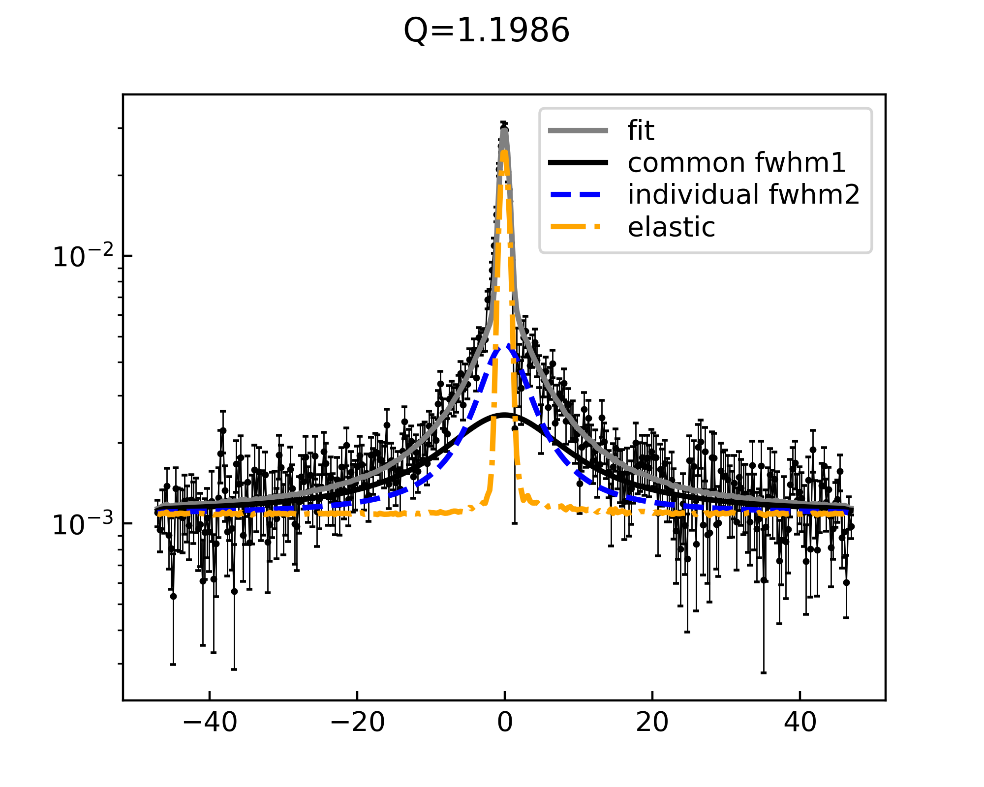
# inspect one of the overall fit
n = 5 # which one to plot
p = js.mplot()
p.Yaxis(scale='log')
p.Title(f'Q={sam[n].Q} ')
p.Plot(sam[n])
p.Plot(sam.lastfit[n], sy=0, li=[1, 2, 14], le='fit')
p.Plot(sam.lastfit[n].X, sam.lastfit[n]._m1, sy=0, li=[1, 2, 10], le='common fwhm1')
p.Plot(sam.lastfit[n].X, sam.lastfit[n]._m2, sy=0, li=[2, 2, 4], le='individual fwhm2')
p.Plot(sam.lastfit[n].X, sam.lastfit[n]._el, sy=0, li=[3, 2, 6], le='elastic')
p.Legend()
# p.Save('inelasticInstruments_simple.png', size=(5, 4), dpi=400)
Look at a dataset of the fit of all together.
The quality of fits depends strongly on your model and this is a simple one.
Fit multiple quasielastic instruments together
A model for incoherent scattering neglecting coherent and maybe some other contributions
We use real data (spheres@MLZ) but a strongly simplified model ignoring rotational diffusion of the protein, D2O contribution and dihedral CH3 motions visible in IN5 data. Therefore the results are yet not to over interpret even if the diffusion coefficient is not bad.
Also counts from background and empty cell might be present.
The intention is to give a relative simple example how to fit different instruments together taking into account the different resolutions and maybe time domain and frequency domain.
The combined fit allows common parameters as diffusion coefficient,fraction of localised motions with same rmsd and tau but still individual amplitudes and backgrounds.
# The intention is to give an example how to fit different instruments together

import jscatter as js
import numpy as np
from jscatter.dynamic import convolve
from jscatter.dynamic import diffusionHarmonicPotential_w, transDiff_w


def readinx(filename, block, l2p, instrument):
    # reusable function for inx reading
    # neutron scatterers use strange data formats like .inx dependent on local contact
    # the blocks start with  number of channels. Spaces (' 562 ') are important to find the starting line.
    # this might dependent on instrument
    data = js.dL(filename,
                 block=block,  # this finds the starting of the blocks of all angles or Q
                 usecols=[1, 2, 3],  # ignore the numbering at each line
                 lines2parameter=l2p)  # catch the parameters at beginning
    for da in data:
        da.channels = da.line_1[0]
        da.Q = da.line_3[0]  # in 1/A
        da.incident_energy = da.line_3[1]  # in meV
        da.temperature = da.line_3[3]  # in K if given
        da.instrument = instrument
    return data

# recover fit of resolution
# see js.dynamic.resolution_w in examples how this was fitted
vana_spheres = js.dL(js.examples.datapath + '/Vana_fitted.inx.gz')
vana_spheres.getfromcomment('modelname')

# read new data
adh = readinx(js.examples.datapath + '/ADH.inx.gz', block=' 563 ', l2p=[-1, -2, -3, -4, -5],instrument='spheres')

# convert to 1/ns
adhf = js.dynamic.convert_e2w(adh, 293, unit='μeV')


def trs_fitmodel(wt, dw, Q, DD, floc, tau, rmsd, A, bgr, instrument):
    """
    Assume NSE data (WASP@ILL) and backscattering (BS) data.
    BS need the convolution with resolution while NSE data are always resolution corrected.

    wt : times from NSE or frequencies from BS
    other input as above

    Here we assume that the resolution measurements are fitted by multiple Gaussians .
    Experimental data can also be used like in other examples
    """
    if instrument in ['spheres','in5']:
        w = wt  # increase w to avoid boundary effects
        # get right Q value of resolution for selected instrument
        if instrument == 'spheres':
            resolutionQ = vana_spheres.filter(Q=Q)[0]
            resolution = js.dynamic.resolution_w(w=w, resolution=resolutionQ)
        elif instrument == 'IN5':
            resolutionQ = vana_IN5.filter(Q=Q)[0]
            resolution = js.dynamic.resolution_w(w=w, resolution=resolutionQ)

        # The model is the same for these instruments

        # localized diffusion in rmsd with tau
        loc = diffusionHarmonicPotential_w(w, Q, tau, rmsd)
        loc.Y = js.dynamic.elastic_w(w).Y * (1 - floc) + floc * loc.Y  # add elastic fraction
        locw = convolve(loc, resolution, normB=True)

        # translational diffusion
        trans = transDiff_w(w, Q, DD)
        transw = convolve(trans, resolution, normB=True)

        transloc = convolve(trans, loc)
        transloc.floc = floc

        res = convolve(transloc, resolution, normB=True)
        # add amplitude and background
        res.Y = A * res.Y + bgr
        res.X = res.X + resolutionQ.w0 + dw

        # append some of the intermediate contributions
        res = res.addColumn(1,A*transw.Y*(1-floc)+bgr)
        res = res.addColumn(1, A * locw.Y * floc + bgr)
        res = res.addColumn(1,resolution.interp(wt)+bgr)
        res.columnname='w;tl;t;l;r'  # name the columns for easier access

    elif instrument == 'JNSE':
        # a NSE machine operating in time domain needs a different model (not yet)
        t = wt
        res = transrotsurf(t, Q, DD, floc, tau, rmsd)

    # interpolate to needed scale points
    return res.interpAll(wt)

# use reduce data for first faster fitting; use all later
adh2 = adhf[1::3]

# fit single dataArray
ad = adh2[-1]
ad.makeErrPlot(yscale='log', title=str(ad.Q) + ' A\S-1')
ad.setlimit(A=[0, 10000], bgr=[0, 10], DD=[0.005, 10], floc=[0.1, 0.9, 0, 1], tau=[0, 2], rmsd=[0, 20],dw=[-2,2])
ad.fit(trs_fitmodel,
       {'A': 90, 'DD': 0.5,'bgr': 1,  'floc': 0.8, 'tau': 0.1, 'rmsd': 1,'dw':0},
       {},
       {'wt': 'X'},
       method='Nelder-Mead',max_nfev=20000)

ad.errplot.plot(ad.lastfit.X,ad.lastfit._t,li=[1,3,2],sy=0,le='trans')
ad.errplot.plot(ad.lastfit.X,ad.lastfit._l,li=[1,3,4],sy=0,le='loc')
ad.errplot.legend()


# fit all together with common DD, floc, rmsd, tau and independent A and bgr
ad5 = adhf[1::3]
ad5.makeErrPlot(yscale='log', title=fr'{str(ad5.Q)} A\S-1',residual='rel')
ad5.setlimit(A=[0, 10000], bgr=[0, 10], DD=[0.005, 10], floc=[0.01, 0.9, 0, 1], tau=[0, 20], rmsd=[0, 20],dw=[-2,2])
ad5.fit(trs_fitmodel,
        {'A': [90], 'DD': 0.05,'bgr': [1],  'floc': 0.8, 'tau': 0.1, 'rmsd': 1,},
        {'dw':[0]},
        {'wt': 'X'},
        max_nfev=20000)

ad5.savelastErrPlot('inelasticInstruments_together.png', size=(2, 1.5), dpi=400)

# check diffusion
ad5.DD
ad5.DD_err

# inspect one of the overall fit
p = js.grace()
p.yaxis(scale='log')
p.title(f'Q={ad5[-1].Q} A\S-1')
p.plot(ad5[-1])
p.plot(ad5.lastfit[-1],sy=0,li=[1,2,14],le='fit')
p.plot(ad5.lastfit[-1].X,ad5.lastfit[-1]._l,sy=0,li=[1,2,10],le='local')
p.plot(ad5.lastfit[-1].X,ad5.lastfit[-1]._t,sy=0,li=[1,2,4],le='diffusion')
p.legend()
p.save('inelasticInstruments_one.png', size=(2, 1.5), dpi=400)
Look at the fit of all together.
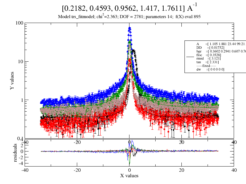
One Q value only
A comparison of different dynamic models in frequency domain
Compare different kinds of diffusion in restricted geometry by the HWHM from the spectra.
import jscatter as js
import numpy as np

# make a plot of the spectrum
w = np.r_[-100:100:1]
ql = np.r_[1:15:.5]
p = js.grace()
p.title('Inelastic neutron scattering ')
p.subtitle('diffusion in a sphere')
iqw = js.dL([js.dynamic.diffusionInSphere_w(w=w, q=q, D=0.14, R=0.2) for q in ql])
p.plot(iqw)
p.yaxis(scale='l', label='I(q,w) / a.u.', min=1e-6, max=1, )
p.xaxis(scale='n', label=r'w / ns\S-1', min=-100, max=100, )

# Parameters
ql = np.r_[0.5:15.:0.2]
D = 0.1
R = 0.5  # diffusion coefficient and radius
w = np.r_[-100:100:0.1]
u0 = R / 4.33 ** 0.5
t0 = R ** 2 / 4.33 / D  # corresponding values for Gaussian restriction, see Volino et al.

# In the following we calc the spectra and then extract the FWHM to plot it

# calc spectra
iqwD = js.dL([js.dynamic.transDiff_w(w=w, q=q, D=D) for q in ql[5:]])
iqwDD = js.dL([js.dynamic.time2frequencyFF(js.dynamic.simpleDiffusion, 'elastic', w=w, q=q, D=D) for q in ql])
iqwS = js.dL([js.dynamic.diffusionInSphere_w(w=w, q=q, D=D, R=R) for q in ql])
iqwG3 = js.dL([js.dynamic.diffusionHarmonicPotential_w(w=w, q=q, rmsd=u0, tau=t0, ndim=3) for q in ql])
iqwG2 = js.dL([js.dynamic.diffusionHarmonicPotential_w(w=w, q=q, rmsd=u0, tau=t0, ndim=2) for q in ql])
iqwG11 = js.dL([js.dynamic.t2fFF(js.dynamic.diffusionHarmonicPotential, 'elastic', w=w, q=q, rmsd=u0,
                                 tau=t0, ndim=1) for q in ql])
iqwG22 = js.dL([js.dynamic.t2fFF(js.dynamic.diffusionHarmonicPotential, 'elastic', w=w, q=q, rmsd=u0,
                                 tau=t0, ndim=2) for q in ql])
iqwG33 = js.dL([js.dynamic.t2fFF(js.dynamic.diffusionHarmonicPotential, 'elastic', w=w, q=q, rmsd=u0,
                                 tau=t0, ndim=3) for q in ql])
# iqwCH3=js.dL([js.dynamic.t2fFF(js.dynamic.methylRotation,'elastic',w=w,q=q ) for q in ql])

# plot HWHM  in a scaled plot
p1 = js.grace(1.5, 1.5)
p1.title('Inelastic neutron scattering models')
p1.subtitle('Comparison of HWHM for different types of diffusion')
p1.plot([0.1, 60], [4.33296] * 2, li=[1, 1, 1], sy=0)
p1.plot((R * iqwD.wavevector.array) ** 2, [js.dynamic.getHWHM(dat)[0] / (D / R ** 2) for dat in iqwD], sy=[1, 0.5, 1],
        le='free')
p1.plot((R * iqwS.wavevector.array) ** 2, [js.dynamic.getHWHM(dat)[0] / (D / R ** 2) for dat in iqwS], sy=[2, 0.5, 3],
        le='in sphere')
p1.plot((R * iqwG3.wavevector.array) ** 2, [js.dynamic.getHWHM(dat)[0] / (D / R ** 2) for dat in iqwG3], sy=[3, 0.5, 4],
        le='harmonic 3D')
p1.plot((R * iqwG2.wavevector.array) ** 2, [js.dynamic.getHWHM(dat)[0] / (D / R ** 2) for dat in iqwG2], sy=[4, 0.5, 7],
        le='harmonic 2D')
p1.plot((R * iqwDD.wavevector.array) ** 2, [js.dynamic.getHWHM(dat)[0] / (D / R ** 2) for dat in iqwDD], sy=0,
        li=[1, 2, 7], le='free fft')
p1.plot((R * iqwG11.wavevector.array) ** 2, [js.dynamic.getHWHM(dat, gap=0.04)[0] / (D / R ** 2) for dat in iqwG11],
        sy=0, li=[1, 2, 1], le='harmonic 1D fft')
p1.plot((R * iqwG22.wavevector.array) ** 2, [js.dynamic.getHWHM(dat, gap=0.04)[0] / (D / R ** 2) for dat in iqwG22],
        sy=0, li=[2, 2, 1], le='harmonic 2D fft')
p1.plot((R * iqwG33.wavevector.array) ** 2, [js.dynamic.getHWHM(dat, gap=0.04)[0] / (D / R ** 2) for dat in iqwG33],
        sy=0, li=[3, 2, 1], le='harmonic 3D fft')
# 1DGauss as given in the reference (see help for this function) seems to have a mistake
# Use the t2fFF from time domain
# p1.plot((0.12*iqwCH3.wavevector.array)**2,[js.dynamic.getHWHM(dat,gap=0.04)[0]/(D/0.12**2) for dat in iqwCH3],
#                                                                             sy=0,li=[1,2,4], le='1D harmonic')


# jump diffusion
r0 = .5
t0 = r0 ** 2 / 2 / D
w = np.r_[-100:100:0.02]
iqwJ = js.dL([js.dynamic.jumpDiff_w(w=w, q=q, r0=r0, t0=t0) for q in ql])
ii = 54
p1.plot((r0 * iqwJ.wavevector.array[:ii]) ** 2, [js.dynamic.getHWHM(dat)[0] / (D / r0 ** 2) for dat in iqwJ[:ii]])
p1.text(r'jump diffusion', x=8, y=1.4, rot=0, charsize=1.25)
p1.plot((R * iqwG33.wavevector.array) ** 2, (R * iqwG33.wavevector.array) ** 2, sy=0, li=[3, 2, 1])
p1.yaxis(min=0.3, max=100, scale='l', label='HWHM/(D/R**2)')
p1.xaxis(min=0.3, max=140, scale='l', label=r'(q*R)\S2')
p1.legend(x=0.35, y=80, charsize=1.25)
# The finite Q resolution results in  js.dynamic.getHWHM (linear interpolation to find [max/2])
# in an offset for very narrow spectra
p1.text(r'free diffusion', x=8, y=10, rot=45, color=2, charsize=1.25)
p1.text(r'free ', x=70, y=65, rot=0, color=1, charsize=1.25)
p1.text(r'3D ', x=70, y=45, rot=0, color=4, charsize=1.25)
p1.text(r'sphere', x=70, y=35, rot=0, color=3, charsize=1.25)
p1.text(r'2D ', x=70, y=15, rot=0, color=7, charsize=1.25)
p1.text(r'1D ', x=70, y=7, rot=0, color=2, charsize=1.25)
p1.save('DynamicModels.png', size=(3, 3), dpi=150)
Protein incoherent scattering in frequency domain
We look at a protein in solution that shows translational and rotational diffusion with atoms local restricted in a harmonic potential.
This is what is expected for the incoherent scattering of a protein (e.g. at 50mg/ml concentration). The contribution of methyl rotation is missing.
- For details see :
Fast internal dynamics in alcohol dehydrogenase, The Journal of Chemical Physics 143, 075101 (2015), https://doi.org/10.1063/1.4928512
Here we use a reading of a PDB structure with only CA atoms for a simple model. This can be improved using the bio module accessing positions and selecting hydrogen atoms or adding coherent scattering.
First we look at the separate contributions :
# A model for protein incoherent scattering
# neglecting coherent and maybe some other contributions

import jscatter as js
import numpy as np
import urllib
from jscatter.dynamic import convolve as conv
from jscatter.dynamic import transDiff_w
from jscatter.dynamic import rotDiffusion_w
from jscatter.dynamic import diffusionHarmonicPotential_w

# get pdb structure file with 3rn3 atom coordinates and filter for CA positions in A
# this results in C-alpha representation of protein Ribonuclease A.
url = 'https://files.rcsb.org/download/3RN3.pdb'
pdbtxt = urllib.request.urlopen(url).read().decode('utf8')
CA = [line[31:55].split() for line in pdbtxt.split('\n') if line[13:16].rstrip() == 'CA' and line[:4] == 'ATOM']
# conversion to nm and center of mass
ca = np.array(CA, float) / 10.
cloud = ca - ca.mean(axis=0)
Dtrans = 0.086  # nm**2/ns  for 3rn3 in D2O at 20°C
Drot = 0.0163  # 1/ns
natoms = cloud.shape[0]

# A list of wavevectors and frequencies and a resolution.
# If bgr is zero we have to add it later after the convolution with resolution as constant instrument background.
# As resolution a single q independent (unrealistic) Gaussian is used.
ql = np.r_[0.1, 0.5, 1, 2:15.:2, 20, 30, 40]
w = np.r_[-100:100:0.1]
start = {'s0': 0.5, 'm0': 0, 'a0': 1, 'bgr': 0.00}
resolution = lambda w: js.dynamic.resolution_w(w=w, **start)
res = resolution(w)

# translational diffusion
p = js.grace(3, 0.75)
p.multi(1, 4)
p[0].title(' ' * 50 + 'Inelastic neutron scattering for protein Ribonuclease A', size=2)

iqwRtr = js.dL([conv(transDiff_w(w, q=q, D=Dtrans), res, normB=True) for q in ql])
iqwRt = js.dL([transDiff_w(w, q=q, D=Dtrans) for q in ql])

p[0].plot(iqwRtr, le='$wavevector')
p[0].plot(iqwRt, li=1, sy=0)
p[0].yaxis(min=1e-8, max=1e3, scale='l', ticklabel=['power', 0, 1], label=[r'I(Q,\xw\f{})', 1.5])
p[0].xaxis(min=-149, max=99, label=r'\xw\f{} / 1/ns', charsize=1)
p[0].legend(charsize=1, x=-140, y=1)
p[0].text(r'translational diffusion, one atom', y=80, x=-130, charsize=1.5)
p[0].text(r'Q / nm\S-1', y=2, x=-140, charsize=1.5)

# rotational diffusion
iqwRr = js.dL([rotDiffusion_w(w, q=q, cloud=cloud, Dr=Drot) for q in ql])
iqwRrr = js.dL([conv(iqw, res, normB=True) for iqw in iqwRr])

p[1].plot(iqwRr, li=1, sy=0)
p[1].plot(iqwRrr, le='$wavevector')
p[1].yaxis(min=1e-8, max=1e3, scale='l', ticklabel=['power', 0, 1, 'normal'])
p[1].xaxis(min=-149, max=99, label=r'\xw\f{} / 1/ns', charsize=1)
# p[1].legend()
p[1].text(r'rotational diffusion full cloud', y=50, x=-130, charsize=1.5)

# restricted diffusion in a harmonic local potential
# rmsd defines the size of the harmonic potential
iqwRgr = js.dL([conv(diffusionHarmonicPotential_w(w, q=q, tau=0.15, rmsd=0.3), res, normB=True) for q in ql])
iqwRg = js.dL([diffusionHarmonicPotential_w(w, q=q, tau=0.15, rmsd=0.3) for q in ql])

p[2].plot(iqwRgr, le='$wavevector')
p[2].plot(iqwRg, li=1, sy=0)
p[2].yaxis(min=1e-8, max=1e3, scale='l', ticklabel=['power', 0, 1], label='')
p[2].xaxis(min=-149, max=99, label=r'\xw\f{} / 1/ns', charsize=1)
# p[2].legend()
p[2].text(r'restricted diffusion one atom \n(harmonic)', y=50, x=-130, charsize=1.5)

# amplitudes at w=0 and w=10
p[3].title('amplitudes w=[0, 10]')
p[3].subtitle(r'\xw\f{}>10 restricted diffusion > translational diffusion')
ww = 10
wi = np.abs(w - ww).argmin()
p[3].plot(iqwRtr.wavevector, iqwRtr.Y.array.max(axis=1) * natoms, sy=[1, 0.3, 1], li=[1, 2, 1], le='trans + res')
p[3].plot(iqwRt.wavevector, iqwRt.Y.array.max(axis=1)* natoms, sy=[1, 0.3, 1], li=[2, 2, 1], le='trans ')
p[3].plot(iqwRt.wavevector, iqwRt.Y.array[:, wi]* natoms, sy=[2, 0.3, 1], li=[3, 3, 1], le='trans w=%.2g' % ww)
p[3].plot(iqwRrr.wavevector, iqwRrr.Y.array.max(axis=1), sy=[1, 0.3, 2], li=[1, 2, 2], le='rot + res')
p[3].plot(iqwRr.wavevector, iqwRr.Y.array.max(axis=1), sy=[1, 0.3, 2], li=[2, 2, 2], le='rot')
p[3].plot(iqwRr.wavevector, iqwRr.Y.array[:, wi], sy=[2, 0.3, 2], li=[3, 3, 2], le='rot w=%.2g' % ww)
p[3].plot(iqwRgr.wavevector, iqwRgr.Y.array.max(axis=1)* natoms, sy=[1, 0.3, 3], li=[1, 2, 3], le='restricted + res')
p[3].plot(iqwRg.wavevector, iqwRg.Y.array.max(axis=1)* natoms, sy=[8, 0.3, 3], li=[2, 2, 3], le='restricted')
p[3].plot(iqwRg.wavevector, iqwRg.Y.array[:, wi]* natoms, sy=[3, 0.3, 3], li=[3, 3, 3], le='restricted w=%.2g' % ww)

p[3].yaxis(min=1e-4, max=5e4, scale='l', ticklabel=['power', 0, 1, 'opposite'],
           label=[r'I(Q,\xw\f{}=[0,10])', 1, 'opposite'])
p[3].xaxis(min=0.1, max=50, scale='l', label=r'Q / nm\S-1', charsize=1)
p[3].legend(charsize=0.9, x=2.8, y=0.057)

p[3].text(r'translation', y=8e-1, x=15, rot=331, charsize=1.3, color=1)
p[3].text(r'rotation', y=6e1, x=15, rot=331, charsize=1.3, color=2)
p[3].text(r'harmonic', y=1e-1, x=15, rot=331, charsize=1.3, color=3)
p[3].text(r'\xw\f{}=10', y=1e-2, x=0.2, rot=30, charsize=1.5, color=1)
p[3].line(0.17, 5e-2, 0.17, 8e-3, 5, arrow=2, color=1)

p[3].text(r'resolution', y=2212, x=0.5, rot=0, charsize=1.5, color=4)

p[3].line(0.5, 100, 0.5, 25, 5, arrow=2, color=4)
p[3].line(0.5, 1500, 0.5, 300, 5, arrow=2, color=4)

p.save('inelasticNeutronScattering.png', size=(6, 1.5), dpi=400)
Blue arrows indicate the effect of instrument resolution at low Q. While rotation is always dominating, at \(\omega=10\) restricted diffusion (harmonic) is stronger than translational diffusion in midrange Q.
Now we add the above components to a combined model.
exR defines a radius from the center of mass that discriminates between fixed hydrogen inside
and hydrogen with additional restricted diffusion outside (close to the protein surface).
start = {'s0': 0.5, 'm0': 0, 'a0': 1, 'bgr': 0.00}
resolution = lambda w: js.dynamic.resolution_w(w=w, **start)


def transrotsurfModel(w, q, Dt, Dr, exR, tau, rmsd):
    """
    A model for trans/rot diffusion with a partial local restricted diffusion at the protein surface.

    See Fast internal dynamics in alcohol dehydrogenase The Journal of Chemical Physics 143, 075101 (2015);
    https://doi.org/10.1063/1.4928512

    Parameters
    ----------
    w   frequencies
    q   wavevector
    Dt  translational diffusion
    Dr  rotational diffusion
    exR outside this radius additional restricted diffusion with t0 u0
    tau  correlation time
    rmsd  Root mean square displacement Ds=u0**2/t0

    Returns
    -------

    """
    natoms = cloud.shape[0]
    trans = transDiff_w(w, q, Dt)
    trans.Y = trans.Y * natoms  # natoms contribute
    rot = rotDiffusion_w(w, q, cloud, Dr)  # already includes natoms
    fsurf = ((cloud ** 2).sum(axis=1) ** 0.5 > exR).sum()  # fraction of natoms close to surface
    loc = diffusionHarmonicPotential_w(w, q, tau, rmsd)
    # only fsurf atoms at surface contributes to local restricted diffusion, others elastic
    loc.Y = js.dynamic.elastic_w(w).Y * (natoms - fsurf) + fsurf * loc.Y

    final = conv(trans, rot)
    final = conv(final, loc)
    final.setattr(rot, 'rot_')
    final.setattr(loc, 'loc_')

    res = resolution(w)
    finalres = conv(final, res, normB=True)

    # finalres.Y+=0.0073  # background ?
    finalres.q = q
    finalres.fsurf = fsurf
    return finalres


ql = np.r_[0.1, 0.5, 1, 2, 4, 6, 10, 20]
p = js.grace(1, 1)
p.title('Protein incoherent scattering')
p.subtitle('Ribonuclease A')
iqwR = js.dL([transrotsurfModel(w, q=q, Dt=Dtrans, Dr=Drot, exR=0, tau=0.15, rmsd=0.3) for q in ql])
p.plot(iqwR[0], sy=0, li=[1, 2, 1], le='exR=0')
p.plot(iqwR[1:], sy=0, li=[1, 2, 1])
iqwR = js.dL([transrotsurfModel(w, q=q, Dt=Dtrans, Dr=Drot, exR=1, tau=0.15, rmsd=0.3) for q in ql])
p.plot(iqwR[0], sy=0, li=[1, 2, 2], le='exR=1')
p.plot(iqwR[1:], sy=0, li=[1, 2, 2])
iqwR = js.dL([transrotsurfModel(w, q=q, Dt=Dtrans, Dr=Drot, exR=1.4, tau=0.15, rmsd=0.3) for q in ql])
p.plot(iqwR[0], sy=0, li=[3, 3, 3], le='exR=1.4')
p.plot(iqwR[1:], sy=0, li=[3, 3, 3])
p.yaxis(min=1e0, max=2e5, label=r'I(q,\xw\f{})', scale='l', ticklabel=['power', 0, 1])
p.xaxis(min=0.1, max=100, label=r'\xw\f{} / ns\S-1', scale='l')
p.legend(x=0.2, y=1e1)

p[0].line(1, 5e2, 1, 5e1, 2, arrow=1)
p.text('resolution', x=0.9, y=7e1, rot=90)
p.text(r'q=2 nm\S-1', x=0.2, y=1e5, rot=0)
p.text(r'q=20 nm\S-1', x=0.2, y=8e2, rot=0)
p.text(r'q=3 nm\S-1', x=2, y=5e4, rot=0)
p.text(r'q=0.1 nm\S-1', x=2.2, y=1.5e2, rot=0)

p[0].line(0.17, 9e4, 0.17, 1e3, 2, arrow=2)
p[0].line(2, 1.5e2, 2, 4e4, 2, arrow=2)
p.text(r'Variation \nfixed/harmonic protons', x=1.2, y=4.44, rot=0)
p[0].line(7, 5.3, 12, 55, arrow=2)

p.save('Ribonuclease_inelasticNeutronScattering.png', size=(4, 4), dpi=150)
We observe that the elastic intensity first increases with Q and decreases again for \(Q>2 nm^{-1}\).
Variation of the fraction of hydrogen that show restricted diffusion is observable for midrange Q.
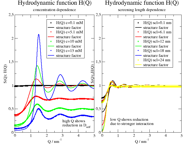
Hydrodynamic function
import numpy as np
import jscatter as js

# Hydrodynamic function and structure factor of hard spheres
# The hydrodynamic function describes how diffusion of spheres in concentrated suspension
# is changed due to hydrodynamic interactions.
# The diffusion is changed according to D(Q)=D0*H(Q)/S(Q)
# with the hydrodynamic function H(Q), structure factor S(Q)
# and Einstein diffusion of sphere D0

# some  wavevectors
q = np.r_[0:5:0.03]

p = js.grace(2, 1.5)
p.multi(1, 2)
p[0].title('Hydrodynamic function H(Q)')
p[0].subtitle('concentration dependence')
Rh = 2.2
for ii, mol in enumerate(np.r_[0.1:20:5]):
    H = js.sf.hydrodynamicFunct(q, Rh, molarity=0.001 * mol, )
    p[0].plot(H, sy=[1, 0.3, ii + 1], legend='H(Q) c=%.2g mM' % mol)
    p[0].plot(H.X, H[3], sy=0, li=[1, 2, ii + 1], legend='structure factor')

p[0].legend(x=2, y=2.4)
p[0].yaxis(min=0., max=2.5, label='S(Q); H(Q)')
p[0].xaxis(min=0., max=5., label=r'Q / nm\S-1')

# hydrodynamic function and structure factor of charged spheres
p[1].title('Hydrodynamic function H(Q)')
p[1].subtitle('screening length dependence')
for ii, scl in enumerate(np.r_[0.1:30:6]):
    H = js.sf.hydrodynamicFunct(q, Rh, molarity=0.0005, structureFactor=js.sf.RMSA,
                                structureFactorArgs={'R': Rh * 2, 'scl': scl, 'gamma': 5}, )
    p[1].plot(H, sy=[1, 0.3, ii + 1], legend='H(Q) scl=%.2g nm' % scl)
    p[1].plot(H.X, H[3], sy=0, li=[1, 2, ii + 1], legend='structure factor')

p[1].legend(x=2, y=2.4)
p[1].yaxis(min=0., max=2.5, label='S(Q); H(Q)')
p[1].xaxis(min=0., max=5., label=r'Q / nm\S-1')

p[0].text(r'high Q shows \nreduction in D\sself', x=3, y=0.22)
p[1].text(r'low Q shows reduction \ndue to stronger interaction', x=0.5, y=0.25)

p.save('HydrodynamicFunction.png')
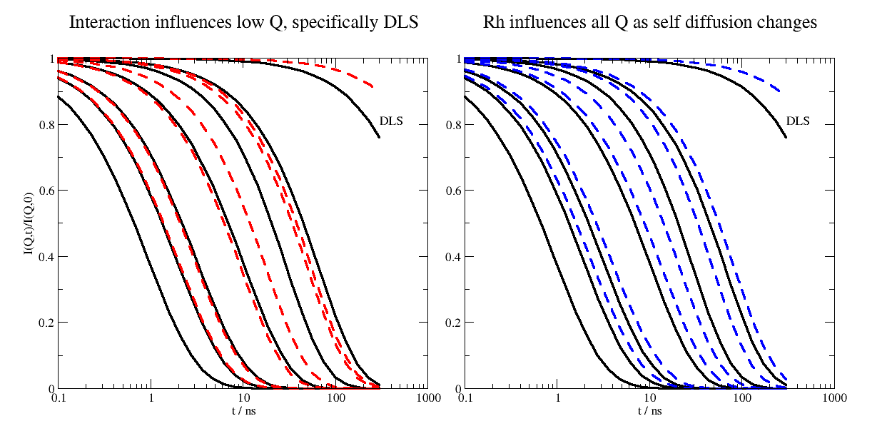
Zimm dynamics including collective effects (H(Q)/S(Q)) on center of mass diffusion
A minimal example how to fit Iqt from NSE measurements on polyelectrolytes using finiteZimm to demonstrate how to include H(Q) and S(Q) for center of mass diffusion Dcm.
For details on the physics see
Interchain Hydrodynamic Interaction and Internal Friction of Polyelectrolytes Buvalaia, et al ACS Macro Letters 12(9):1218 https://doi.org/10.1021/acsmacrolett.3c00409
import jscatter as js
import numpy as np

# the structure factor type and parameters should be determined by fitting of SAXS/SANS data
# only for simplicity we use the PercusYevick, molarity is determined by experimental conditions of NSE
# here the experimental R of the PercusYevick is determined from experimental data

q0 = np.r_[0.01:2:100j]


def collectivefiniteZIMM(t, q, Dt=None, mu=0.5, Rh=4, R=4,tint=0, mol=0.0003):
    # Hq can be determined integrating over Sq and using Rh as a fit parameter
    # We assume here a polymer with different hydrodynamic interaction compared to a sphere
    # internally SF is calculated and saved in _sf
    SF = js.sf.PercusYevick
    HqSq = js.sf.hydrodynamicFunct(q0, Rh=Rh, molarity=mol,
                                 structureFactor=SF,
                                 structureFactorArgs={'R': R}, )
    HqSq.Y =  HqSq.Y / HqSq._sf  # this makes the needed H(Q)/S(Q)
    hqsq = HqSq[:2]  # only first columns

    # Dt is determined inside finiteZimm , but can be changed
    Iqt = js.dynamic.finiteZimm(t, q, NN=212, pmax=25, l=0.24, Dcm=Dt, tintern=tint, Temp=273 + 60, mu=mu,
                                viscosity=1, Dcmfkt = hqsq)
    Iqt.setColumnIndex(iey=None)
    return Iqt


# simulate data, typical NSE times IN15@ILL
tlist = js.loglist(0.1,300,30)

p = js.grace(2,1)
p.multi(1,2)
p[0].xaxis(label='t / ns',scale='log')
p[1].xaxis(label='t / ns',scale='log')
p[0].yaxis(label='I(Q,t)/I(Q,0)')

# lowest Q corresponds to DLS as synthetic dataset added to Iqt from NSE
sim = js.dL()
for q in np.r_[0.026,0.25,0.4,0.8,1.2,1.4,1.8]:  # in 1/nm
    sim.append(collectivefiniteZIMM(t=tlist, q=q, mol=0.0003, R=8, Rh=4, mu=0.6))
p[0].plot(sim,sy=0,li=[1,3,1])
p[1].plot(sim,sy=0,li=[1,3,1])

sim2 = js.dL()
for q in np.r_[0.026,0.25,0.4,0.6,0.8,1.2,1.4]:  # in 1/nm
    sim2.append(collectivefiniteZIMM(t=tlist, q=q, mol=0.0003, R=7, Rh=4, mu=0.6))
p[0].plot(sim2,sy=0,li=[3,3,2])

sim3 = js.dL()
for q in np.r_[0.026,0.25,0.4,0.6,0.8,1.2,1.4]:  # in 1/nm
    sim3.append(collectivefiniteZIMM(t=tlist, q=q, mol=0.0003, R=8, Rh=6, mu=0.6))
p[1].plot(sim3,sy=0,li=[3,3,4])

p[0].text('DLS',x=300,y=0.8)
p[1].text('DLS',x=300,y=0.8)
p[0].title('Interaction influences low Q, specifically DLS')
p[1].title('Rh influences all Q as self diffusion changes')

# p.save('collectiveZimm.png', size=(2, 1), dpi=150)

if 0:
    # A fit to exp. NSE data might be done like this (using sim as measured data, no errors)
    # fixpar are determined from other experiments
    sim.fit(model=collectivefiniteZIMM,
                freepar={'Rh':4,'mu':0.6,'tint':1},
                fixpar={'R':6, 'mol':0.0003 },  # from exp. conditions
                mapNames={'t':'X'})
Checkout the structure factor and HqSq to examine the Q dependent changes in the center of mass diffusion.