Analysis of SAS data

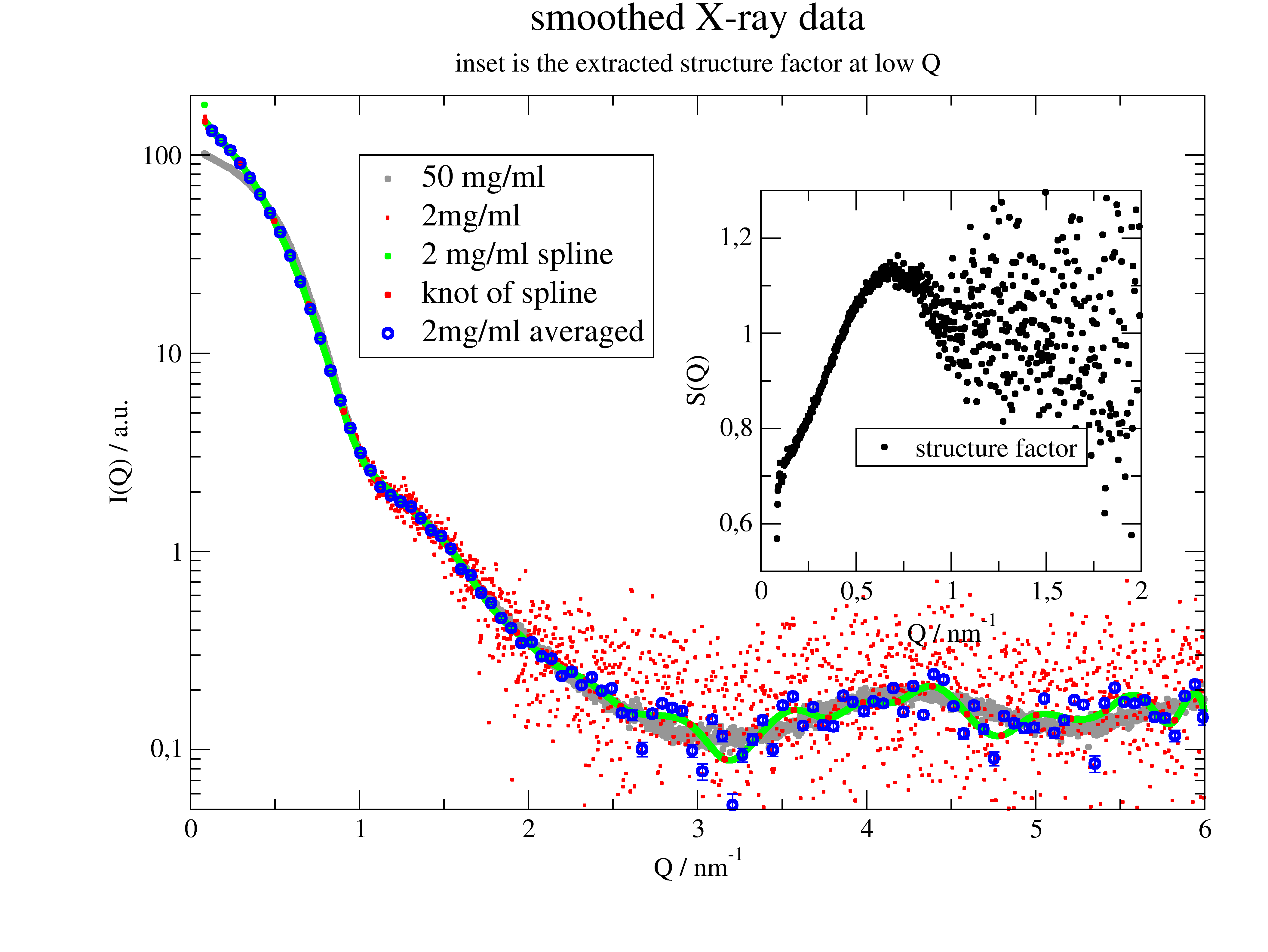
How to smooth Xray data and make an inset in the plot

SAS data often have a large number of points at higher Q. The best way to get reasonable statistics there is to reduce the number of points by averaging in intervals (see .prune). Spline gives trust less results.

These are real data from X33 beamline, EMBL Hamburg.

import jscatter as js
import numpy as np
from scipy.interpolate import LSQUnivariateSpline

# load data
ao50 = js.dA(js.examples.datapath + '/a0_336.dat')
ao50.conc = 50
ao10 = js.dA(js.examples.datapath + '/a0_338.dat')
ao10.conc = 2

p = js.grace(1.5, 1)
p.clear()

p.plot(ao50.X, ao50.Y, symbol=[1, 0.2, 9], legend='50 mg/ml')
p.plot(ao10.X, ao10.Y, line=0, symbol=[1, 0.05, 2], legend='2mg/ml')
p.xaxis(0, 6, label=r'Q / nm\S-1')
p.yaxis(0.05, 200, scale='logarithmic', label='I(Q) / a.u.')
p.title('smoothed X-ray data')
p.subtitle('inset is the extracted structure factor at low Q')

# smoothing with a spline
# determine the knots of the spline 
# less points than data points
t = np.r_[ao10.X[1]:ao10.X[-2]:30j]
# calculate the spline
f = LSQUnivariateSpline(ao10.X, ao10.Y, t)
# calculate the new y values of the spline at the x points
ys = f(ao10.X)
p.plot(ao10.X, ys, symbol=[1, 0.2, 5, 5], legend='2 mg/ml spline ')
p.plot(t, f(t), line=0, symbol=[1, 0.2, 2, 1], legend='knot of spline')

# other idea: use lower number of points with averages in intervals
# this makes 100 intervals with average X and Y values and errors if wanted. Check prune how to use it!
# this is the best solution and additionally creates good error estimate!!!
p.plot(ao10.prune(number=100), line=0, symbol=[1, 0.5, 4], legend='2mg/ml averaged')
p.legend(x=1, y=100, charsize=1.2)
p.xaxis(0, 6)
p.yaxis(0.05, 200, scale='logarithmic')

# make a smaller plot inside for the structure factor
p.new_graph()
p[1].SetView(0.6, 0.4, 0.9, 0.8)
p[1].plot(ao50.X, ao50.Y / ao10.Y, symbol=[1, 0.2, 1, ''], legend='structure factor')
p[1].yaxis(0.5, 1.3, label='S(Q)')
p[1].xaxis(0, 2, label=r'Q / nm\S-1')
p[1].legend(x=0.5, y=0.8)

p.save('smooth_xraydata.png')

Analysis of SAS data

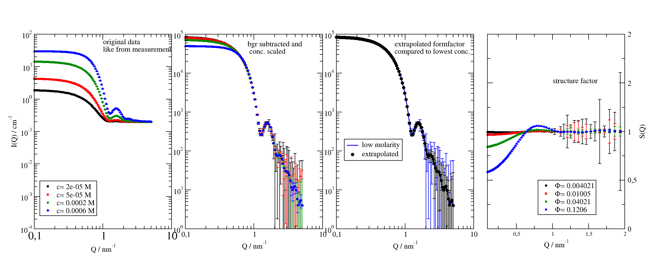
In small angle scattering a typical situation is that you want to measure a formfactor (particle shape) or structure factor (particle interaction). For this a concentration series is measured and we need to extrapolate to zero concentration to get the formfactor. Afterwards we can divide the measurement by the formfactor to get the structure factor. So we have three key parts :

• Correction for transmission, dark and empty cell scattering to get instrument independent datasets.

• Extrapolating concentration scaled data to get the formfactor.

• Divide by formfactor to get structure factor

Correction

Brulet at al [1] describe the data correction for SANS, which is in principle also valid for SAXS, if incoherent contributions are neglected.

The difference is, that SAXS has typical transmission around ~0.3 for 1mm water sample in quartz cell due to absorption, while in SANS typical values are around ~0.9 for D2O. Larger volume fractions in the sample play a more important rule for SANS as hydrogenated ingredients reduce the transmission significantly, while in SAXS still the water and the cell (quartz) dominate.

One finds for a sample inside of a container with thicknesses (\(z\)) for sample, buffer (solvent), empty cell and empty beam measurement (omitting the overall q dependence):

\[I_s = \frac{1}{z_S}\big((\frac{I_S-I_{dark}}{T_S}-I_{b}T_S\big) -\big(\frac{I_{EC}-I_{dark}}{T_{EC}}-I_{b}T_{EC})\big) - \frac{1}{z_B}\big((\frac{I_B-I_{dark}}{T_B}-I_{b}T_B\big) -\big(\frac{I_{EC}-I_{dark}}{T_{EC}}-I_{b}T_{EC})\big)\]

where

• \(I_s\) is the interesting species

• \(I_S\) is the sample of species in solvent (buffer)

• \(I_B\) is the pure solvent (describing a constant background)

• \(I_{dark}\) is the dark current measurement. For Pilatus detectors equal zero.

• \(I_b\) is the empty beam measurement

• \(I_{EC}\) is the empty cell measurement

• \(z_x\) corresponding sample thickness

• \(T_x\) corresponding transmission

The recurring pattern \(\big((\frac{I-I_{dark}}{T}-I_{b}T\big)\) shows that the the beam tail (border of primary beam not absorbed by the beam stop) is attenuated by the corresponding sample.

For equal sample thickness \(z\) the empty beam is included in subtraction of \(I_B\) :

\[I_s = \frac{1}{z} \big((\frac{I_S-I_{dark}}{T_S}-I_{b}T_S) - (\frac{I_B-I_{dark}}{T_B}-I_{b}T_B)\big)\]

• The simple case

  If the transmissions are nearly equal as for e.g. protein samples with low concentration (\(T_S \approx T_B\)) we only need to subtract the transmission and dark current corrected buffer measurement from the sample.

  \[I_s = \frac{1}{z} \big((\frac{I_S-I_{dark}}{T_S}) - (\frac{I_B-I_{dark}}{T_B}\big)\]

• Higher accuracy for large volume fractions

  For larger volume fractions \(\Phi\) the transmission might be different and we have to take into account that only \(1-\Phi\) of solvent contributes to \(I_S\). We may incorporate this in the sense of an optical density changing the effective thickness \(\frac{1}{z_B}\rightarrow\frac{1-\Phi}{z_B}\) resulting in different thicknesses \(z_S \neq z_B\)

[1]

Improvement of data treatment in small-angle neutron scattering Brûlet et al Journal of Applied Crystallography 40, 165-177 (2007)

Extrapolation and dividing by concentration

We assume that the above correction was correctly applied and we have a transmission corrected sample and buffer (background) measurement. This is what you typically get from SANS instruments as e.g KWS1-3 from MLZ Garching or D11-D33 at ILL, Grenoble.

The key part is dataff=datas.extrapolate(molarity=0)[0] to extrapolate to zero molarity.

# Analyse SAS data by extrapolating the form factor followed by structure factor determination

import jscatter as js
import numpy as np

# generate some synthetic data just for this demonstration
# import the model described in example_buildComplexModel
# it describes ellipsoids with PercusYevick structure factor
from jscatter.examples import particlesWithInteraction as PWI

NN = 100
q = js.loglist(0.1, 5, NN)
data = js.dL()
bgr = js.dA(np.c_[q, 0.2 + np.random.randn(NN) * 1e-3, [1e-3] * NN].T)  # background
for m in [0.02, 0.05, 0.2, 0.6]:
    pwi = PWI(q, Ra=3, Rb=4, molarity=m * 1e-3, bgr=0, contrast=6e-4)
    pwi = pwi.addColumn(1, np.random.randn(NN) * 1e-3)
    pwi.Y = pwi.Y + bgr.Y
    pwi.setColumnIndex(iey=-1)
    data.append(pwi)

# With measured data the above is just reading data and background
# with an attribute molarity or concentration.
# This might look like this
if 0:
    data = js.dL()
    bgr = js.dA('backgroundmeasurement.dat')
    for name in ['data_conc01.dat', 'data_conc02.dat', 'data_conc05.dat', 'data_conc08.dat']:
        data.append(name)
        data[-1].molarity = float(name.split('.')[0][-2:])

p = js.grace(2, 0.8)
p.multi(1, 4)
p[0].plot(data, sy=[-1, 0.3, -1], le='c= $molarity M')
p[0].yaxis(min=1e-4, max=1e2, scale='l', label=r'I(Q) / cm\S-1', tick=[10, 9], charsize=1, ticklabel=['power', 0, 1])
p[0].xaxis(scale='l', label=r'Q / nm\S-1', min=1e-1, max=1e1, charsize=1)
p[0].text(r'original data\nlike from measurement', y=50, x=1)
p[0].legend(x=0.12, y=0.003)

# Using the synthetic data we extract again the form factor and structure factor
# subtract background and scale data by concentration or volume fraction
datas = data.copy()
for dat in datas:
    dat.Y = (dat.Y - bgr.Y) / dat.molarity
    dat.eY = (dat.eY + bgr.eY) / dat.molarity  # errors increase
p[1].plot(datas, sy=[-1, 0.3, -1], le='c= $molarity M')
p[1].yaxis(min=1, max=1e5, scale='l', tick=[10, 9], charsize=1, ticklabel=['power', 0])
p[1].xaxis(scale='l', label=r'Q / nm\S-1', min=1e-1, max=1e1, charsize=1)
p[1].text(r'bgr subtracted and\n conc. scaled', y=5e4, x=0.8)

# extrapolate to zero concentration to get the  form factor
# dataff=datas.extrapolate(molarity=0,func=lambda y:-1/y,invfunc=lambda y:-1/y)
dataff = datas.extrapolate(molarity=0)[0]
# as error *estimate* we may use the mean of the errors which is not absolutely correct
dataff = dataff.addColumn(1, datas.eY.array.mean(axis=0))
dataff.setColumnIndex(iey=2)
p[2].plot(datas[0], li=[1, 2, 4], sy=0, le='low molarity')
p[2].plot(dataff, sy=[1, 0.5, 1, 1], le='extrapolated')
p[2].yaxis(min=1, max=1e5, scale='l', tick=[10, 9], charsize=1, ticklabel=['power', 0])
p[2].xaxis(scale='l', label=r'Q / nm\S-1', min=1e-1, max=1e1, charsize=1)
p[2].legend(x=0.13, y=200)
p[2].text(r'extrapolated formfactor \ncompared to lowest conc.', y=5e4, x=0.7)

# calc the structure factor by dividing by the form factor
sf = datas.copy()
for dat in sf:
    dat.Y = dat.Y / dataff.Y
    dat.eY = (dat.eY ** 2 / dataff.Y ** 2 + dataff.eY ** 2 * (dat.Y / dataff.Y ** 2) ** 2) ** 0.5
    dat.volfrac = dat.Volume * dat.molarity
p[3].plot(sf, sy=[-1, 0.3, -1], le=r'\xF\f{}= $volfrac')
p[3].yaxis(min=0, max=2, scale='n', label=['S(Q)', 1, 'opposite'], charsize=1, ticklabel=['General', 0, 1, 'opposite'])
p[3].xaxis(scale='n', label=r'Q / nm\S-1', min=1e-1, max=2, charsize=1)
p[3].text('structure factor', y=1.5, x=1)
p[3].legend(x=0.8, y=0.5)

# remember so safe the form factor and structurefactor
# sf.save('uniquenamestructurefactor.dat')
# dataff.save('uniquenameformfactor.dat')

# save the figures
p.save('SAS_sf_extraction.agr')
p.save('SAS_sf_extraction.png', size=(2500/300, 1000/300), dpi=300)

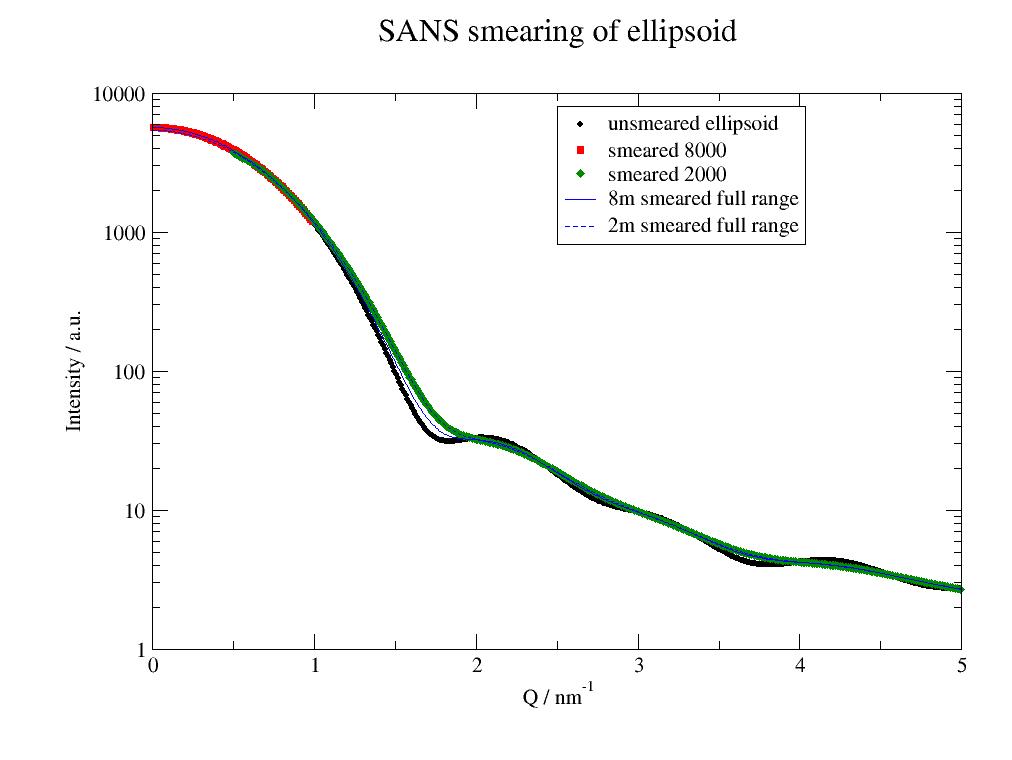
How to fit SANS data including the resolution for different detector distances

First this example shows the influence of smearing, then how to do a fit including

smearing a la Pedersen. The next example can do the same.

import jscatter as js
import numpy as np

# prepare profiles SANS for typical 2m and 8m measurement
# smear calls resFunc with the respective parameters; smear also works with line collimation SAXS if needed
resol8m = js.sas.prepareBeamProfile('SANS', collDist=8000., collAperture=10, detDist=8000., sampleAperture=10,
                                    wavelength=0.5, wavespread=0.2, dpixelWidth=10, dringwidth=1)


# demonstration smearing effects

# define model and use @smear to wrap it with the smearing function
# detDist and collDist will be used in js.sas.smear to change the beamprofile for smearing

@js.sas.smear(beamProfile=resol8m)
def ellipsoid(q, a, b, bgr, detDist=2000, collDist=2000.):
    elli = js.ff.ellipsoid(q, a, b)
    elli.Y = elli.Y + bgr
    return elli


# generate some smeared data, or load them from measurement
a, b = 2, 3
data = js.dL()
data.append(ellipsoid(np.r_[0.01:1:0.01], a, b, 2, detDist=8000, collDist=8000.))
data.append(ellipsoid(np.r_[0.5:5:0.05], a, b, 2, detDist=2000, collDist=2000.))

# here we compare the difference between the 2 profiles using for both the full q range
data2 = js.dL()
data2.append(ellipsoid(np.r_[0.01:5:0.02], a, b, 2, detDist=8000, collDist=8000.))
data2.append(ellipsoid(np.r_[0.01:5:0.02], a, b, 2, detDist=2000, collDist=2000.))

# plot it
p = js.grace()
ellip = js.ff.ellipsoid(np.r_[0.01:5:0.01], a, b)
ellip.Y += 2
p.plot(ellip, sy=[1, 0.3, 1], legend='unsmeared ellipsoid')
p.yaxis(label='Intensity / a.u.', scale='l', min=1, max=1e4)
p.xaxis(label=r'Q / nm\S-1', scale='n')
p.plot(data, legend='smeared $rf_detDist')
p.plot(data2[0], li=[1, 1, 4], sy=0, legend='8m smeared full range')
p.plot(data2[1], li=[3, 1, 4], sy=0, legend='2m smeared full range')
p.legend(x=2.5, y=8000)
p.title('SANS smearing of ellipsoid')
p.save('SANSsmearing.jpg')

# now we use the simulated data to fit this to a model
# the data need attributes detDist and collDist to use correct parameters in smearing
# here we add these from above in rf_detDist (set in smear)
# for a measurement this needs to be added to the experimental data
data[0].detDist = data[0].rf_detDist
data[0].collDist = data[0].rf_collDist
data[1].detDist = data[1].rf_detDist
data[1].collDist = data[1].rf_collDist


@js.sas.smear(beamProfile=resol8m)
def smearedellipsoid(q, A, a, b, bgr, detDist=2000, collDist=2000.):
    """
    The model may use all needed parameters for smearing.
    """
    ff = js.ff.ellipsoid(q, a, b)  # calc model
    ff.Y = ff.Y * A + bgr  # multiply amplitude factor and add bgr
    return ff


# fit it , here no errors
data.makeErrPlot(yscale='l', fitlinecolor=[1, 2, 5])
data.fit(smearedellipsoid, {'A': 1, 'a': 2.5, 'b': 3.5, 'bgr': 0}, {}, {'q': 'X'})
# show the unsmeared model
p = js.grace()
for oo in data:
    p.plot(oo, sy=[-1, 0.5, -1], le='lastfit smeared')
    p.plot(oo.X, oo[2], li=[3, 2, 4], sy=0, legend='lastfit unsmeared')
p.yaxis(scale='l')
p.legend()
p.save('SANSsmearingFit.jpg')

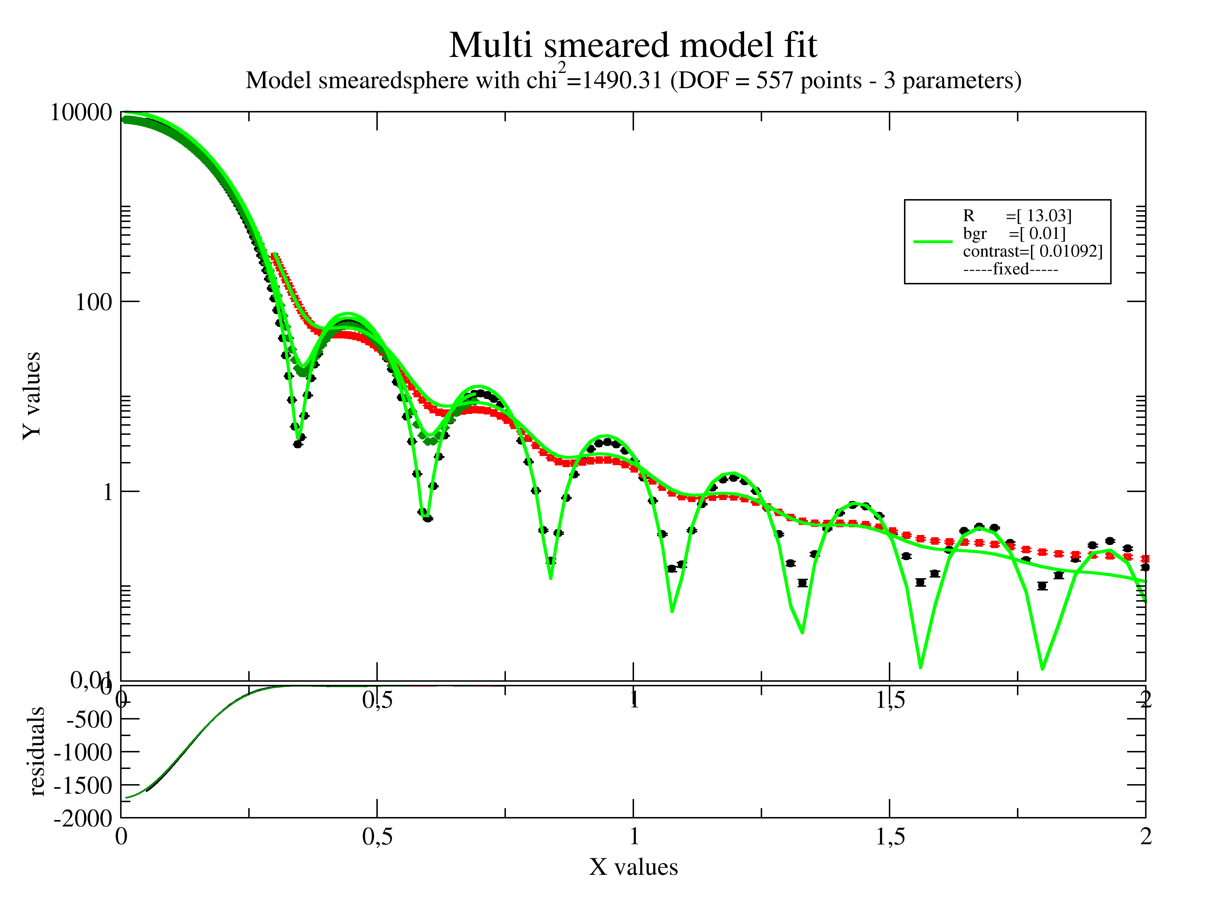
Fitting multiple smeared data together

In the following example all smearing types may be mixed and can be fitted together. For details and more examples on smearing see smear()

This examples shows SAXS/SANS smearing with different collimation.

import jscatter as js
import numpy as np

# prepare beamprofiles according to measurement setup
# SAXS with small resolution
fbeam = js.sas.prepareBeamProfile(0.01)
# low and high Q SANS
Sbeam4m = js.sas.prepareBeamProfile('SANS', detDist=4000, wavelength=0.4, wavespread=0.1)
Sbeam20m = js.sas.prepareBeamProfile('SANS', detDist=20000, wavelength=0.4, wavespread=0.1)


# define smeared model with beamProfile as parameter
@js.sas.smear(beamProfile=fbeam)
def smearedsphere(q, R, bgr, contrast=1, beamProfile=None):
    sp = js.ff.sphere(q=q, radius=R, contrast=contrast)
    sp.Y = sp.Y + bgr
    return sp


# read data with 3 measurements
smeared = js.dL(js.examples.datapath+'/smearedSASdata.dat')

# add corresponding smearing to the datasets
# that the model can see in attribute beamprofile how to smear
smeared[0].beamProfile = fbeam
smeared[1].beamProfile = Sbeam4m
smeared[2].beamProfile = Sbeam20m

if 0:
    # For scattering data it is sometimes advantageous
    # to use a log weight in fit using the error weight
    for temp in smeared:
        temp.eY = temp.eY *np.log(temp.Y)

# fit it
smeared.setlimit(bgr=[0.01])
smeared.makeErrPlot(yscale='l', fitlinecolor=[1, 2, 5], title='Multi smeared model fit')
smeared.fit(smearedsphere, {'R': 12, 'bgr': 0.1, 'contrast': 1e-2}, {}, {'q': 'X'})
# smeared.errplot.save(js.examples.imagepath+'/smearedfitexample.png')

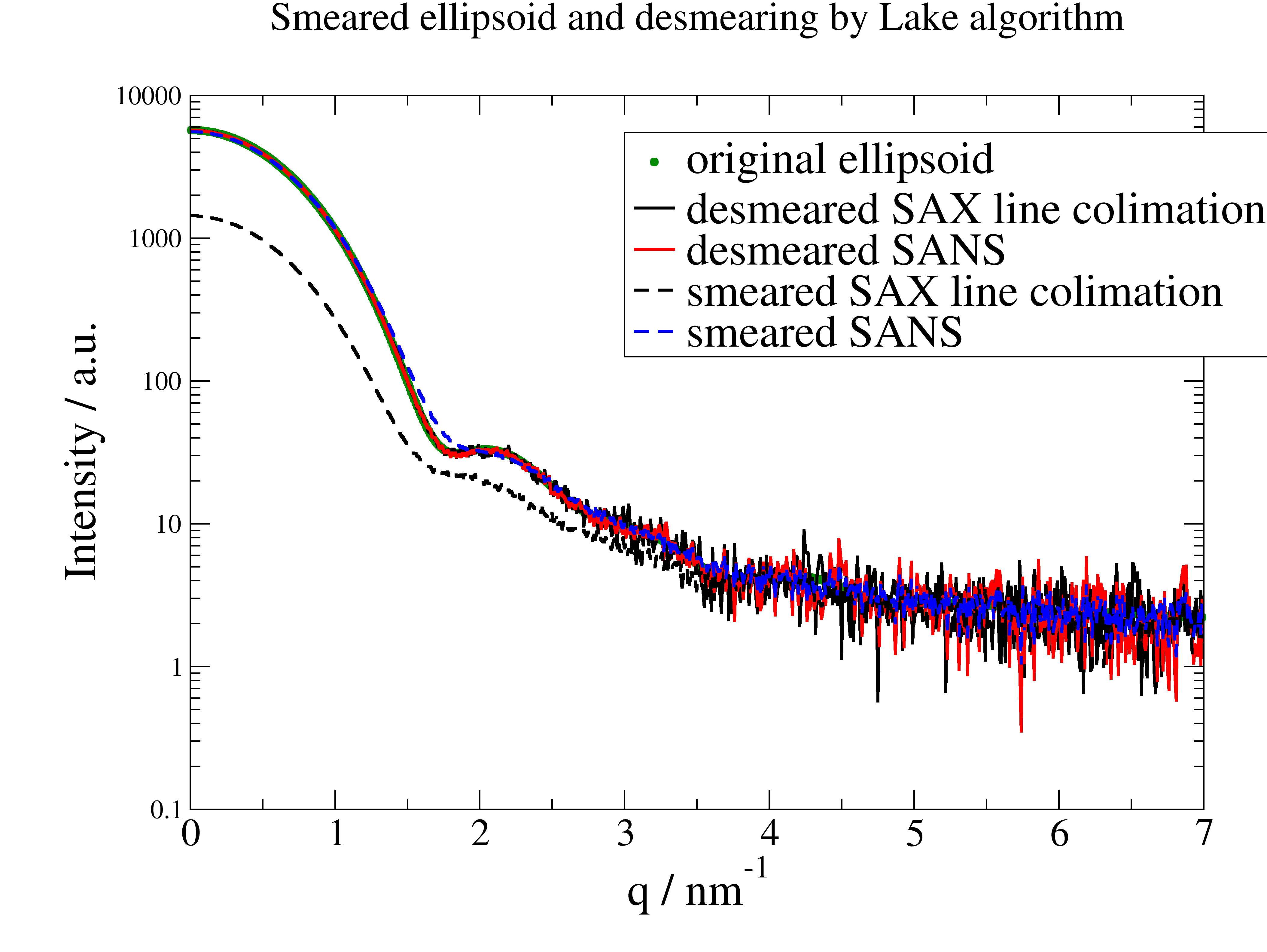
Smearing and desmearing of SAX and SANS data

Here we examine the effect of instrumental smearing for SAX (Kratky Camera, line! ) and SANS and how we can use the Lake algorithm for desmearing.

The conclusion is that because of the increased noise it is in most cases more effective to fit smeared models than to desmear data and fit these. The additional advantage is that at the edges (eg detector limits) we can desmear a model correctly while we need assumptions for the data (e.g. low Q Guinier behavior, high Q as constant) which are sometimes difficult to justify.

import jscatter as js
import numpy as np

# Here we examine the effect of instrumental smearing for SAX (Kratky Camera, line! ) and SANS
# and how we can use the Lake algorithm for desmearing.

# some data
q = np.r_[0.01:7:0.01]
# obj = js.ff.sphere(q,5)
data = js.ff.ellipsoid(q, 2, 3)
# add background
data.Y += 2
# load data for beam width profile
empty = js.dA(js.examples.datapath + '/buffer_averaged_corrected_despiked.pdh', usecols=[0, 1],
              lines2parameter=[2, 3, 4])
# read beam length profile measurement for a slit (Kratky Camera)
beam = js.dA(js.examples.datapath + '/BeamProfile.pdh', usecols=[0, 1], lines2parameter=[2, 3, 4])

# fit beam width for line collimation with semitransparent beam stop
bwidth = js.sas.getBeamWidth(empty, 'auto')

# prepare measured beamprofile from beam measurement
mbeam = js.sas.prepareBeamProfile(beam, a=2, b=1, bxw=bwidth, dIW=1.)
# prepare profile with trapezoidal shape using explicit given parameters (using parameters from above to have equal)
tbeam = js.sas.prepareBeamProfile('trapez', a=mbeam.a, b=mbeam.b, bxw=bwidth, dIW=1)
# prepare profile SANS a la Pedersen in point collimation. This can be used for SAXS with smaller apertures too!
Sbeam = js.sas.prepareBeamProfile('SANS', detDist=2000, wavelength=0.4, wavespread=0.15)

if 0:
    p = js.sas.plotBeamProfile(mbeam)
    p = js.sas.plotBeamProfile(mbeam, p)

# smear
datasm = js.sas.smear(unsmeared=data, beamProfile=mbeam)
datast = js.sas.smear(unsmeared=data, beamProfile=tbeam)
datasS = js.sas.smear(unsmeared=data, beamProfile=Sbeam)
# add noise
datasm.Y += np.random.normal(0, 0.5, len(datasm.X))
datast.Y += np.random.normal(0, 0.5, len(datast.X))
datasS.Y += np.random.normal(0, 0.5, len(datasS.X))

# desmear again
ws = 11
NI = -15
dsm = js.sas.desmear(datasm, mbeam, NIterations=NI, windowsize=ws)
dst = js.sas.desmear(datast, tbeam, NIterations=NI, windowsize=ws)
dsS = js.sas.desmear(datasS, Sbeam, NIterations=NI, windowsize=ws)

# compare
p = js.grace(2, 1.4)
p.plot(data, sy=[1, 0.3, 3], le='original ellipsoid')
p.plot(dst, sy=0, li=[1, 2, 1], le='desmeared SAX line collimation')
p.plot(dsS, sy=0, li=[1, 2, 2], le='desmeared SANS')
p.plot(datasm, li=[3, 2, 1], sy=0, le='smeared SAX line collimation')
p.plot(datasS, li=[3, 2, 4], sy=0, le='smeared SANS')
p.yaxis(max=1e4, min=0.1, scale='l', label='Intensity / a.u.', size=1.7)
p.xaxis(label=r'q / nm\S-1', size=1.7)
p.legend(x=3, y=5500, charsize=1.7)
p.title('Smeared ellipsoid and desmearing by Lake algorithm')

# The conclusion is to better fit smeared models than to desmear and fit unsmeared models.
p.save('SASdesmearing.png')

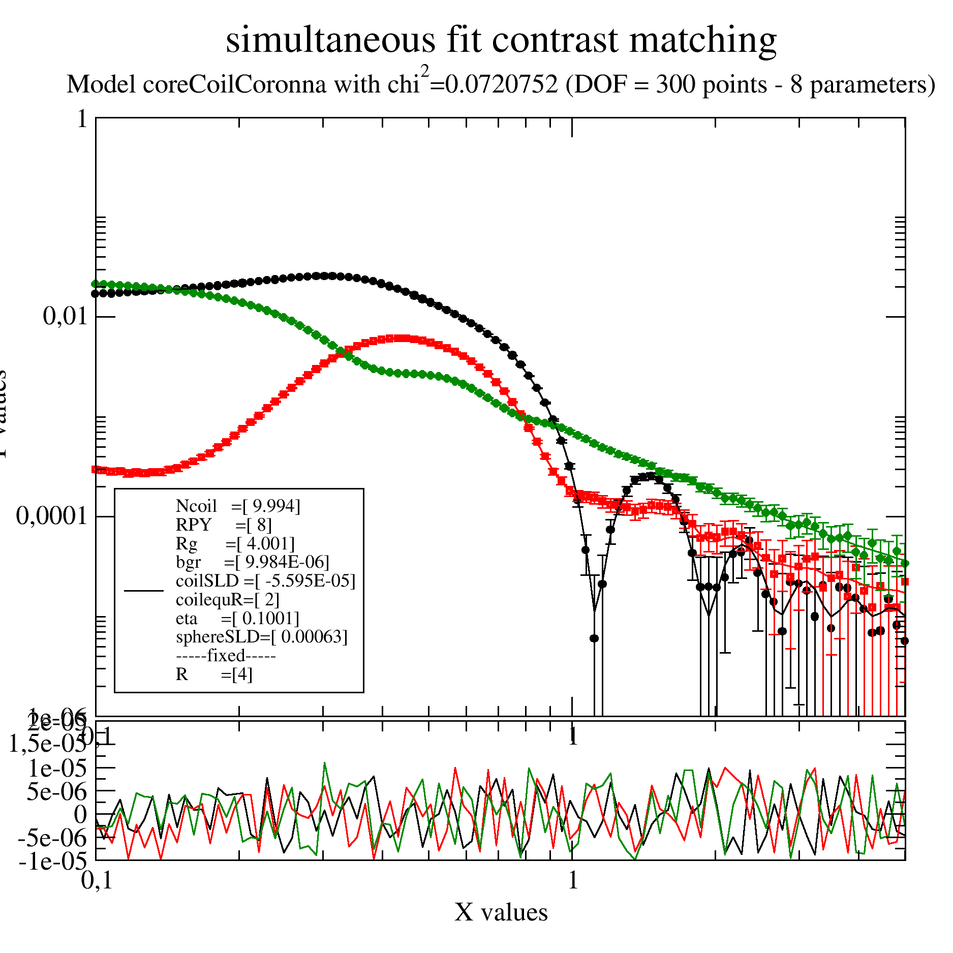
Simultaneous fit SANS data of a partly matched sample measured at 3 contrast conditions

In this example we ignore smearing (Add it if needed).

We have a sample like a micelles of a diblock copolymer with a shorter hydrophobic and a longer hydrophilic part. The hydrophobic part will make a core with hydrophilic extended Gaussian coils into the solvent.

To separate core and coils 3 contrast were measured in H2O, a H2O/D2O mixture with SLD 3e-4 and D2O.

As a reasonable high concentration was used we observe in the core contrast (black points) already a structure factor as a maximum at around 0.3 /nm. The minimum around 1 /nm defines the core radius in ths contrast that we fix. This structure factor we need to include.

We do a simultaneous fit of all together using the coreGaussiancoronna model. To add structure factor and background we write our own model.

import jscatter as js

# read data measured at 3 contrast conditions:
i5 = js.dL(js.examples.datapath + '/gauscoronna.dat')
# add solvent contrast to data from preparation, will be used as fixed parameter per dataArray
i5[0].solventSLD = -0.56e-4    # H2O contrast (nearly its actually lower, but this is just an example)
i5[1].solventSLD = 3e-4        # some H2O/D2O mixture
i5[2].solventSLD = 6.3e-4      # D2O
i5.setlimit(bgr=[0, 0.00001], RPY=[0, 20])


# define sphereGaussianCorona with background
def coreCoilCoronna(q, R, Ncoil, Nmonomer, monomerVolume, a, coilSLD, sphereSLD, solventSLD, RPY,eta,bgr):
    res = js.ff.sphereGaussianCorona(q, R=R, Ncoil=Ncoil,Nmonomer=Nmonomer,monomerVolume=monomerVolume,a=a ,
                                     coilSLD=coilSLD, sphereSLD=sphereSLD, solventSLD=solventSLD)
    res.Y =res.Y * js.sf.PercusYevick(q, RPY, eta=eta).Y + bgr
    return res


# make ErrPlot to see progress of intermediate steps with residuals (updated all 2 seconds)
i5.makeErrPlot(title='simultaneous fit contrast matching', xscale='log', yscale='log', legpos=[0.12, 0.5])

# fit it
# the minimum in core contrast can be used to predetermine "R":4
# Method 'Nelder-Mead' searches more for a solution,direct use of 'lm' works here
i5.fit(model=coreCoilCoronna,  # the fit function
       freepar={ 'Ncoil': 8, 'Nmonomer':100,
                 'coilSLD': 3e-4, 'sphereSLD': 3e-4, 'bgr': 0, 'RPY':7,'eta':0.1},
       fixpar={'R': 4, 'a':0.8, 'monomerVolume':0.12},
       mapNames={'q': 'X', })

# use a 'lm' to polish the result and get errors using the last fit result as start
# here this really improves the fit
i5.estimateError()

# i5.errplot.save(js.examples.imagepath+'/multicontrastfit.png', size=(1.5, 1.5))

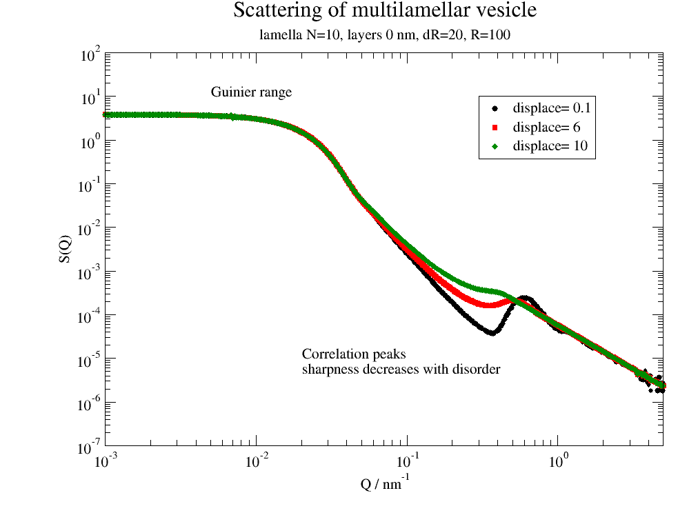
Multilamellar Vesicles

Here we look at the various effects appearing for vesicles and how they change the scattering.

import jscatter as js

Q = js.loglist(0.001, 5, 500)  # np.r_[0.01:5:0.01]

ffmV = js.ff.multilamellarVesicles
save = 0

# correlation peak sharpness depends on disorder
dR = 20
nG = 200
p = js.grace(1, 1)
for dd in [0.1, 6, 10]:
    p.plot(ffmV(Q=Q, R=100, displace=dd, dR=dR, N=10, dN=0, phi=0.2, nGauss=nG),
           le='displace= %g ' % dd)

p.legend(x=0.3, y=10)
p.title('Scattering of multilamellar vesicle')
p.subtitle('lamella N=10, layerd 0 nm, dR=20, R=100')
p.yaxis(label='S(Q)', scale='l', min=1e-7, max=1e2, ticklabel=['power', 0])
p.xaxis(label=r'Q / nm\S-1', scale='l', min=1e-3, max=5, ticklabel=['power', 0])
p.text('Guinier range', x=0.005, y=10)
p.text(r'Correlation peaks\nsharpness decreases with disorder', x=0.02, y=0.00001)
if save: p.save('multilamellar1.png')

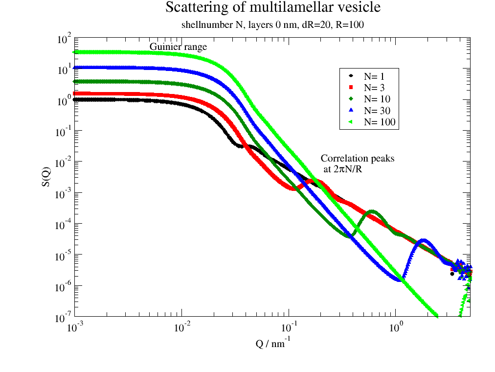
# Correlation peak position depends on average layer distance
dd = 0
dR = 20
nG = 200
p = js.grace(1, 1)
for N in [1, 3, 10, 30, 100]:
    p.plot(ffmV(Q=Q, R=100, displace=dd, dR=dR, N=N, dN=0, phi=0.2, nGauss=nG), le='N= %g ' % N)

p.legend(x=0.3, y=10)
p.title('Scattering of multilamellar vesicle')
p.subtitle('shellnumber N, layers 0 nm, dR=20, R=100')
p.yaxis(label='S(Q)', scale='l', min=1e-7, max=1e2, ticklabel=['power', 0])
p.xaxis(label=r'Q / nm\S-1', scale='l', min=1e-3, max=5, ticklabel=['power', 0])

p.text('Guinier range', x=0.005, y=40)
p.text(r'Correlation peaks\n at 2\xp\f{}N/R', x=0.2, y=0.01)
if save: p.save('multilamellar2.png')

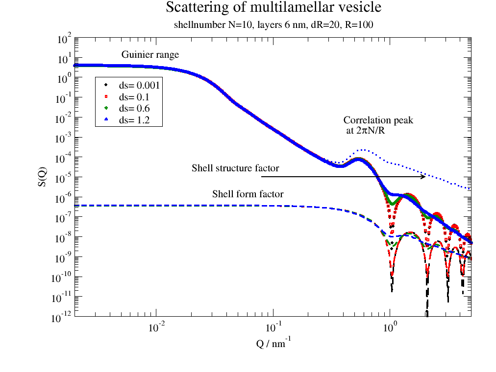
# including the shell formfactor with fluctuations of layer thickness
dd = 2
dR = 20
nG = 200
p = js.grace(1, 1)
# multi lamellar structure factor
mV = ffmV(Q=Q, R=100, displace=dd, dR=dR, N=10, dN=0, phi=0.2, layerd=6, layerSLD=1e-4, nGauss=nG)
for i, ds in enumerate([0.001, 0.1, 0.6, 1.2], 1):
    # calc layer fomfactor
    lf = js.formel.pDA(js.ff.multilayer, ds, 'layerd', q=Q, layerd=6, layerSLD=1e-4)
    p.plot(mV.X, mV._Sq * lf.Y / lf.Y[0], sy=[i, 0.3, i], le='ds= %g ' % ds)
    p.plot(mV.X, lf.Y, sy=0, li=[3, 3, i])
    p.plot(mV.X, mV._Sq, sy=0, li=[2, 3, i])

p.legend(x=0.003, y=1)
p.title('Scattering of multilamellar vesicle')
p.subtitle('shellnumber N=10, layers 6 nm, dR=20, R=100')
p.yaxis(label='S(Q)', scale='l', min=1e-12, max=1e2, ticklabel=['power', 0])
p.xaxis(label=r'Q / nm\S-1', scale='l', min=2e-3, max=5, ticklabel=['power', 0])

p.text('Guinier range', x=0.005, y=10)
p.text(r'Correlation peak\n at 2\xp\f{}N/R', x=0.4, y=5e-3)
p.text('Shell form factor', x=0.03, y=1e-6)
p.text(r'Shell structure factor', x=0.02, y=2e-5)
p[0].line(0.08, 1e-5, 2, 1e-5, 2, arrow=2)
if save: p.save('multilamellar3.png')

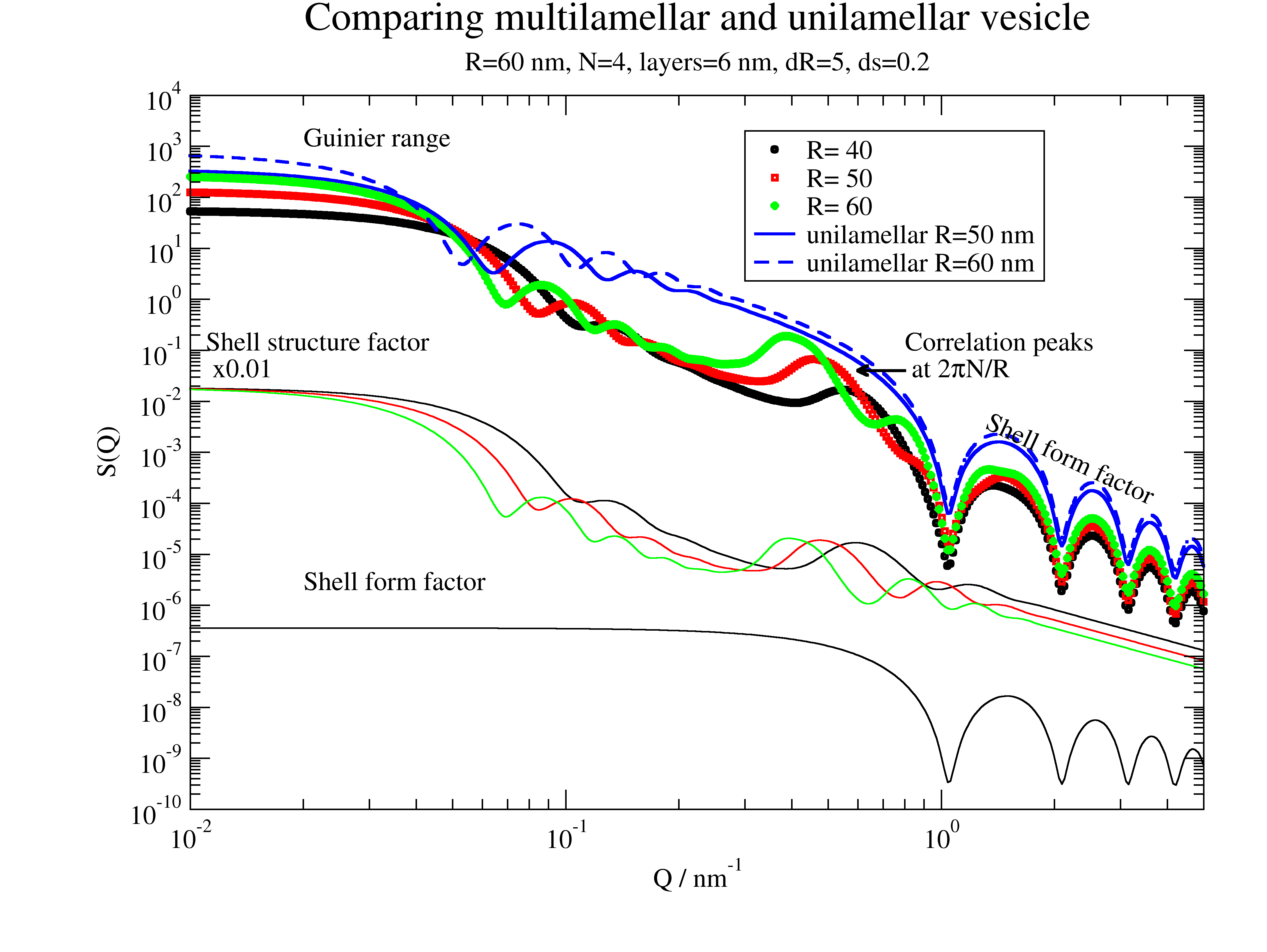
# Comparing multilamellar and unilamellar vesicle
dd = 2
dR = 5
nG = 100
ds = 0.2
N = 4
p = js.grace(1, 1)
for i, R in enumerate([40, 50, 60], 1):
    mV = ffmV(Q=Q, R=R, displace=dd, dR=dR, N=N, dN=0, phi=0.2, layerd=6, ds=ds, layerSLD=1e-4, nGauss=nG)
    p.plot(mV, sy=[i, 0.3, i], le='R= %g ' % R)
    p.plot(mV.X, mV[-2] * 0.01, sy=0, li=[1, 1, i])
# is same for all
p.plot(mV.X, mV[-1], sy=0, li=[1, 1, 1])

# comparison double sphere
mV = ffmV(Q=Q, R=50., displace=0, dR=5, N=1, dN=0, phi=1, layerd=6, ds=ds, layerSLD=1e-4, nGauss=100)
p.plot(mV, sy=0, li=[1, 2, 4], le='unilamellar R=50 nm')
mV = ffmV(Q=Q, R=60., displace=0, dR=5, N=1, dN=0, phi=1, layerd=6, ds=ds, layerSLD=1e-4, nGauss=100)
p.plot(mV, sy=0, li=[3, 2, 4], le='unilamellar R=60 nm')

p.legend(x=0.3, y=2e3)
p.title('Comparing multilamellar and unilamellar vesicle')
p.subtitle(f'R={R} nm, N={N}, layers={6} nm, dR={dR}, ds={ds}')
p.yaxis(label='S(Q)', scale='l', min=1e-10, max=1e4, ticklabel=['power', 0])
p.xaxis(label=r'Q / nm\S-1', scale='l', min=1e-2, max=5, ticklabel=['power', 0])

p.text('Guinier range', x=0.02, y=1000)
p.text(r'Correlation peaks\n at 2\xp\f{}N/R', x=0.8, y=0.1)
p[0].line(0.8, 4e-2, 0.6, 4e-2, 2, arrow=2)
p.text('Shell form factor', x=1.3, y=0.3e-2, rot=335)
# p[0].line(0.2,4e-5,0.8,4e-5,2,arrow=2)
p.text(r'Shell structure factor\n x0.01', x=0.011, y=0.1, rot=0)
p.text('Shell form factor ', x=0.02, y=2e-6, rot=0)
if save: p.save('multilamellar4.png')

The first image shows how a multilamellar vesicles changes the shape of the membrane correlation peak with increasing dislocations of the centers.

Larger number of lamella shifts the correlation peak to higher Q.

The shell formfactor determines the high Q minima. This allows to access the structure of e.g. bilayers.

Multilamellar and unilamellar can be distinguished with the aid of the appearing correlation peaks. See below.

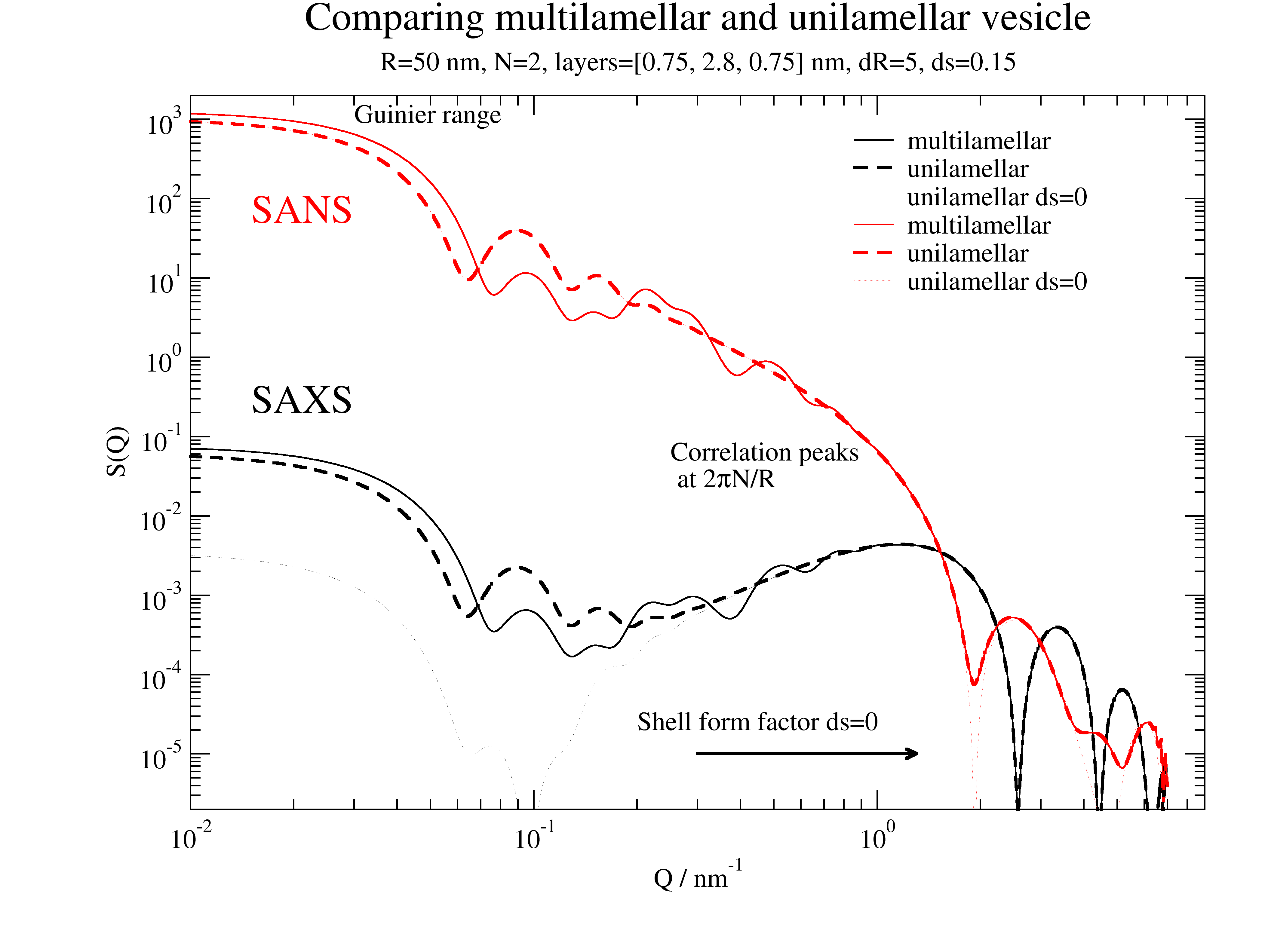
DPPC Vesicle in SAXS

A more realistic example for DPPC We use a simplified model with 3 box layers and approximate thickness and scattering length densities. Kučerka uses a multi Gaussian profile.

# Values for layer thickness can be found in
# Structure of lipid bilayers
# John F. Nagle et al. Biochim Biophys Acta. 1469, 159–195. (2000)

# scattering length densities of head groups and tails
# Small-Angle Neutron Scattering for Studying Lipid Bilayer Membranes
# William T Heller, Biomolecules 2022 Oct 29;12(11):1591.   doi: 10.3390/biom12111591.
#
# phospholipid headgroups (HG) in 1e-4 nm^2
# PC HG           1.877
# 2H18-PC HG      7.736
# PE HG           2.483
# PA HG           2.494
# PG HG (in H2O)  2.382
# PG HG (in2H2O)  3.076
# PS HG (in H2O)  3.466
# PS HG (in2H2O)  3.893
#
# acyl chains in phospholipids in 1e-4 nm^2
# lauroyl (12:0)         -0.386
# 2H23-lauroyl (12:0)     6.755
# myristoyl (14:0)       -0.375
# 2H27-myristoyl (14:0)   6.837
# palmitoyl (16:0)       -0.386
# 2H31-palmitoyl (16:0)   6.557
# oleoyl (18:1c)         -0.386
#
# cholesterol (in H2O)    0.216
# cholesterol (in2H2O)    0.386


import jscatter as js
import numpy as np

ffmV = js.ff.multilamellarVesicles
save = 0

Q = js.loglist(0.01, 7, 500)
dd = 1.5
dR = 5
nG = 100
ds = 0.05  # variation of hydrocarbon layer thickness
R = 50
sd = [0.75, 2.8, 0.75]
N = 2

p = js.grace(1.4,1)
p.title('Multilamellar/unilamellar vesicle for SAXS/SANS')
# SAXS
sld = np.r_[420, 290, 420] * js.formel.felectron  # unit e/nm³*fe
sSLD = 335 * js.formel.felectron  # H2O unit e/nm³*fe
saxm = ffmV(Q=Q, R=R, displace=dd, dR=dR, N=N, dN=0, phi=0.2, layerd=sd, ds=ds, layerSLD=sld, solventSLD=sSLD, nGauss=nG)
p.plot(saxm, sy=0, li=[1, 1, 1], le='multilamellar')
saxu = ffmV(Q=Q, R=R, displace=0, dR=dR, N=1, dN=0, phi=0.2, layerd=sd, ds=ds, layerSLD=sld, solventSLD=sSLD, nGauss=100)
p.plot(saxu, sy=0, li=[3, 2, 1], le='unilamellar')
saxu0 = ffmV(Q=Q, R=R, displace=0, dR=dR, N=1, dN=0, phi=0.2, layerd=sd, ds=0, layerSLD=sld, solventSLD=sSLD, nGauss=100)
p.plot(saxu0, sy=0, li=[2, 0.3, 1], le='unilamellar ds=0')
p.text('SAXS', x=0.015, y=0.2, charsize=1.5,color=1)

# SANS
sld = [1.877e-4, -.375e-4, 1.877e-4]  # unit 1/nm²
sSLD = 6.335e-4  # D2O
sanm = ffmV(Q=Q, R=R, displace=dd, dR=dR, N=N, dN=0, phi=0.2, layerd=sd, ds=ds, layerSLD=sld, solventSLD=sSLD, nGauss=nG)
p.plot(sanm, sy=0, li=[1, 1, 2], le='multilamellar')
sanu = ffmV(Q=Q, R=R, displace=0, dR=dR, N=1, dN=0, phi=0.2, layerd=sd, ds=ds, layerSLD=sld, solventSLD=sSLD, nGauss=100)
p.plot(sanu, sy=0, li=[3, 2, 2], le='unilamellar')
sanu = ffmV(Q=Q, R=R, displace=0, dR=dR, N=1, dN=0, phi=0.2, layerd=sd, ds=0, layerSLD=sld, solventSLD=sSLD, nGauss=100)
p.plot(sanu, sy=0, li=[2, 0.3, 2], le='unilamellar ds=0')
p.text('SANS', x=0.015, y=50, charsize=1.5,color=2)

p.legend(x=0.8, y=950, boxcolor=0, boxfillpattern=0)
p.subtitle('R=%.2g nm, N=%.1g, layerd=%s nm, dR=%.1g, ds=%.2g' % (R, N, sd, dR, ds))

p.yaxis(label='S(Q)', scale='l', min=2e-6, max=2e3, ticklabel=['power', 0])
p.xaxis(label=r'Q / nm\S-1', scale='l', min=1e-2, max=9, ticklabel=['power', 0])
p.text(r'Correlation peaks\n at 2\xp\f{}N/R', x=0.25, y=0.05, charsize=1.,color=1)
p.text('Guinier range', x=0.03, y=900, charsize=1.)
p.text('Shell form factor ds=0', x=0.2, y=0.2e-4)
p[0].line(0.3, 1e-5, 1.3, 1e-5, 2, arrow=2)
if save: p.save('multilamellar5.png')

We observe in this figure modulations at the left flank of the prominent peak. The modulations are caused by the multilamelarity and a clear indication. Already small modulations indicate multi lamellar vesicles in accordance with Kučerka et al.

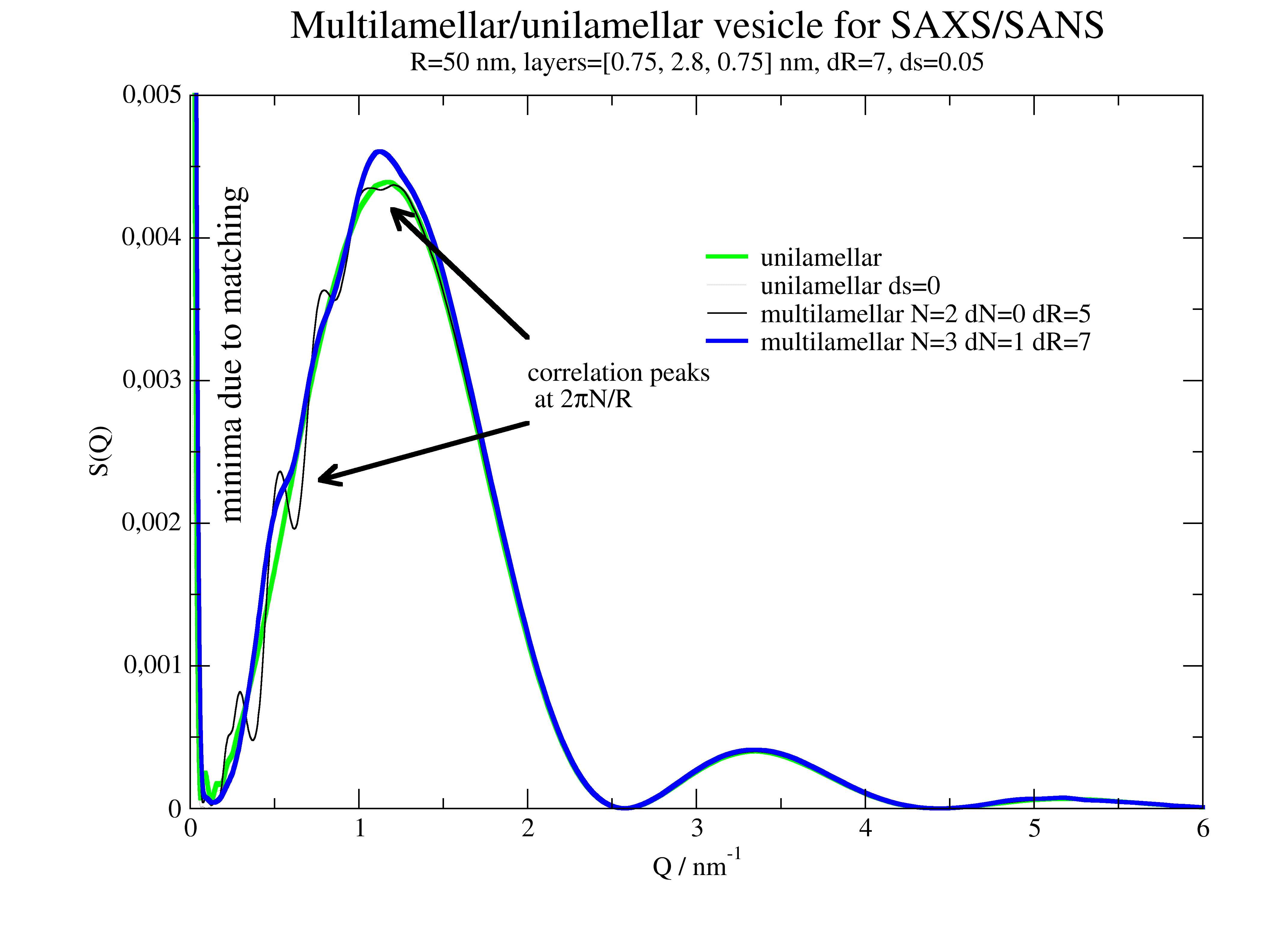
Multilamellar SAXS example for DPPC

The first minima with following increase is a result of the near matching condition for bilayers in SAXS. Additionally we observe characteristic peaks/shoulders in the first increase/top as a result of multilamellar interference. See for comparison Kučerka et al. Langmuir 23, 1292 (2007) https://doi.org/10.1021/la062455t .

We use again the simplified model with 3 box layers and approximate thickness from above

# Values for layer thickness can be found in
# Structure of lipid bilayers
# John F. Nagle et al.Biochim Biophys Acta. 1469, 159–195. (2000)

# scattering length densities of DPPC for SAXS and SANS can be found in
#  Kučerka et al. Biophysical Journal. 95,2356 (2008)
#  https://doi.org/10.1529/biophysj.108.132662

import jscatter as js
import numpy as np

ffmV = js.ff.multilamellarVesicles
save = 0

Q = js.loglist(0.01, 7, 500)
dd = 1.5
dR = 5
nG = 100
ds = 0.05  # variation of hydrocarbon layer thickness
R = 50
sd = [0.75, 2.8, 0.75]
N = 2

p = js.grace(1.4,1)
p.title('Multilamellar/unilamellar vesicle for SAXS/SANS')

# SAXS
sld = np.r_[420, 290, 420] * js.formel.felectron  # unit e/nm³*fe
sSLD = 335 * js.formel.felectron  # H2O unit e/nm³*fe
saxu = ffmV(Q=Q, R=R, displace=0, dR=dR, N=1, dN=0, phi=0.2, layerd=sd, ds=ds, layerSLD=sld, solventSLD=sSLD, nGauss=100)
saxu0 = ffmV(Q=Q, R=R, displace=0, dR=dR, N=1, dN=0, phi=0.2, layerd=sd, ds=0, layerSLD=sld, solventSLD=sSLD, nGauss=100)

p.plot(saxu, sy=0, li=[1, 3, 3], le='unilamellar')
p.plot(saxu0, sy=0, li=[2, 0.3, 1], le='unilamellar ds=0')
N=2; dN=0; dR=5
saxm = ffmV(Q=Q, R=R, displace=dd, dR=dR, N=N, dN=0, phi=0.2, layerd=sd, ds=ds, layerSLD=sld, solventSLD=sSLD, nGauss=nG)
p.plot(saxm, sy=0, li=[1, 1, 1], le=f'multilamellar N={N} dN={dN} dR={dR}')
N=3; dN=1; dR=6
saxm = ffmV(Q=Q, R=R, displace=dd, dR=dR, N=N, dN=dN, phi=0.2, layerd=sd, ds=ds, layerSLD=sld, solventSLD=sSLD, nGauss=nG)
p.plot(saxm, sy=0, li=[1, 3, 4], le=f'multilamellar N={N} dN={dN} dR={dR}')


p.legend(x=3, y=0.004, boxcolor=0, boxfillpattern=0)
p.subtitle('R=%.2g nm, layers=%s nm, dR=%.1g, ds=%.2g' % (R, sd, dR, ds))
p.yaxis(label='S(Q)', scale='n', min=0.0, max=5e-3)
p.xaxis(label=r'Q / nm\S-1', scale='n', min=0, max=6)
p.text(r'correlation peaks\n at 2\xp\f{}N/R', x=2, y=0.003, charsize=1., color=1)
p[0].line(0.77,0.0023,2,2.7e-3, 3,1,1,1,2,2)
p[0].line(1.2,0.0042,2,3.3e-3, 3,1,1,1,2,2)
p.text(r'minima due to matching', x=0.3, y=0.002, charsize=1.3, rot=90)

if save: p.save('multilamellar5SAXS.png')

2D oriented scattering

Formfactors of oriented particles or particle complexes

import jscatter as js
import numpy as np

# Examples for scattering of 2D scattering of some spheres oriented in space relative to incoming beam
# incoming beam along Y
# detector plane X,Z
# For latter possibility to fit 2D data we have Y=f(X,Z)

# two points
rod0 = np.zeros([2, 3])
rod0[:, 1] = np.r_[0, np.pi]
qxz = np.mgrid[-6:6:50j, -6:6:50j].reshape(2, -1).T
ffe = js.ff.orientedCloudScattering(qxz, rod0, mosaicity=[10,0,0], nCone=10, rms=0)
fig = js.mpl.surface(ffe.X, ffe.Z, ffe.Y)
fig.axes[0].set_title('cos**2 for Z and slow decay for X')
fig.show()
# noise in positions
ffe = js.ff.orientedCloudScattering(qxz, rod0, mosaicity=[10,0,0], nCone=100, rms=0.1)
fig = js.mpl.surface(ffe.X, ffe.Z, ffe.Y)
fig.axes[0].set_title('cos**2 for Y and slow decay for X with position noise')
fig.show()
#
# two points along z result in symmetric pattern around zero
# asymmetry is due to small nCone and reflects the used Fibonacci lattice
rod0 = np.zeros([2, 3])
rod0[:, 2] = np.r_[0, np.pi]
ffe = js.ff.orientedCloudScattering(qxz, rod0, mosaicity=[45,0,0], nCone=10, rms=0.05)
fig2 = js.mpl.surface(ffe.X, ffe.Z, ffe.Y)
fig2.axes[0].set_title('symmetric around zero')
fig2.show()
#
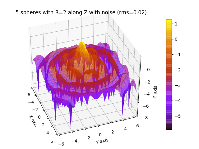
# 5 spheres in line with small position distortion
rod0 = np.zeros([5, 3])
rod0[:, 1] = np.r_[0, 1, 2, 3, 4] * 3
qxz = np.mgrid[-6:6:50j, -6:6:50j].reshape(2, -1).T
ffe = js.ff.orientedCloudScattering(qxz, rod0, formfactoramp='sphere', V=4 / 3. * np.pi * 2 ** 3, mosaicity=[20,0,0],
                                    nCone=30, rms=0.02)
fig4 = js.mpl.surface(ffe.X, ffe.Z, np.log10(ffe.Y), colorMap='gnuplot')
fig4.axes[0].set_title('5 spheres with R=2 along Z with noise (rms=0.02)')
fig4.show()
#
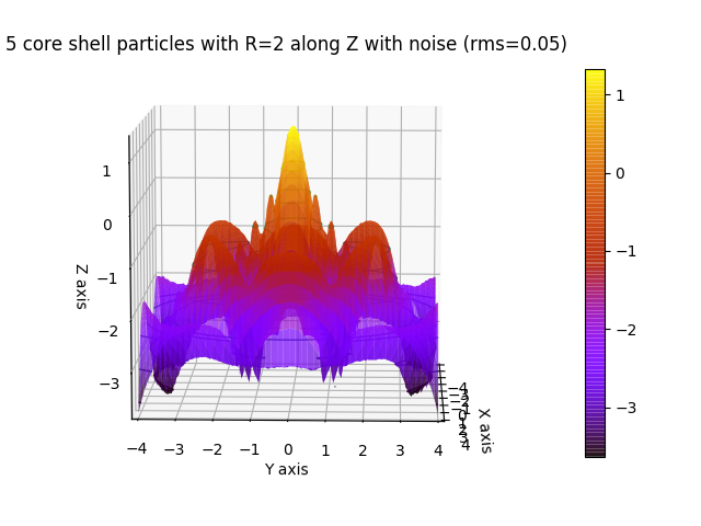
# 5 core shell particles in line with small position distortion (Gaussian)
rod0 = np.zeros([5, 3])
rod0[:, 1] = np.r_[0, 1, 2, 3, 4] * 3
qxz = np.mgrid[-6:6:50j, -6:6:50j].reshape(2, -1).T
# only as demo : extract q from qxz
qxzy = np.c_[qxz, np.zeros_like(qxz[:, 0])]
qrpt = js.formel.xyz2rphitheta(qxzy)
q = np.unique(sorted(qrpt[:, 0]))
# or use interpolation
q = js.loglist(0.01, 7, 100)
# explicitly given isotropic form factor amplitude
cs = js.ff.sphereCoreShell(q=q, Rc=1, Rs=2, bc=0.1, bs=1, solventSLD=0)[[0, 2]]
ffe = js.ff.orientedCloudScattering(qxz, rod0, formfactoramp=cs, mosaicity=[20,0,0], nCone=100, rms=0.05)
fig4 = js.mpl.surface(ffe.X, ffe.Z, np.log10(ffe.Y), colorMap='gnuplot')
fig4.axes[0].set_title('5 core shell particles with R=2 along Z with noise (rms=0.05)')
fig4.show()

# Extracting 1D data
# 1. average angular region (similar to experimental detector data)
# 2. direct calculation
# Here with higher resolution to see the additional peaks due to alignment.
#
# 1:
rod0 = np.zeros([5, 3])
rod0[:, 1] = np.r_[0, 1, 2, 3, 4] * 3
qxz = np.mgrid[-4:4:150j, -4:4:150j].reshape(2, -1).T
# only as demo : extract q from qxz
qxzy = np.c_[qxz, np.zeros_like(qxz[:, 0])]
qrpt = js.formel.xyz2rphitheta(qxzy)
q = np.unique(sorted(qrpt[:, 0]))
# or use interpolation
q = js.loglist(0.01, 7, 100)
cs = js.ff.sphereCoreShell(q=q, Rc=1, Rs=2, bc=0.1, bs=1, solventSLD=0)[[0, 2]]
ffe = js.ff.orientedCloudScattering(qxz, rod0, formfactoramp=cs, mosaicity=[20,0,0], nCone=100, rms=0.05)
fig4 = js.mpl.surface(ffe.X, ffe.Z, np.log10(ffe.Y), colorMap='gnuplot')
fig4.axes[0].set_title('5 core shell particles with R=2 along Z with noise (rms=0.05)')
fig4.show()
#
# transform X,Z to spherical coordinates
qphi = js.formel.xyz2rphitheta([ffe.X, ffe.Z, abs(ffe.X * 0)], transpose=True)[:, :2]
# add qphi or use later rp[1] for selection
ffb = ffe.addColumn(2, qphi.T)
# select a portion of the phi angles
phi = np.pi / 2
dphi = 0.2
ffn = ffb[:, (ffb[-1] < phi + dphi) & (ffb[-1] > phi - dphi)]
ffn.isort(-2)  # sort along radial q
p = js.grace()
p.plot(ffn[-2], ffn.Y, le='oriented spheres form factor')
# compare to coreshell formfactor scaled
p.plot(cs.X, cs.Y ** 2 / cs.Y[0] ** 2 * 25, li=1, le='coreshell form factor')
p.yaxis(label='F(Q,phi=90°+-11°)', scale='log')
p.title('5 aligned core shell particle with additional interferences', size=1.)
p.subtitle(' due to sphere alignment dependent on observation angle')

# 2: direct way with 2D q in xz plane
rod0 = np.zeros([5, 3])
rod0[:, 1] = np.r_[0, 1, 2, 3, 4] * 3
x = np.r_[0.0:6:0.05]
qxzy = np.c_[x, x * 0, x * 0]
for alpha in np.r_[0:91:30]:
    R = js.formel.rotationMatrix(np.r_[0, 0, 1], np.deg2rad(alpha))  # rotate around Z axis
    qa = np.dot(R, qxzy.T).T[:, :2]
    ffe = js.ff.orientedCloudScattering(qa, rod0, formfactoramp=cs, mosaicity=[20,0,0], nCone=100, rms=0.05)
    p.plot(x, ffe.Y, li=[1, 2, -1], sy=0, le='alpha=%g' % alpha)
p.xaxis(label=r'Q / nm\S-1')
p.legend()
p.save('5alignedcoreshellparticlewithadditionalinterferences.png')

Oriented crystal structure factors in 2D

# Comparison of different domain sizes dependent on direction of scattering ::

import jscatter as js
import numpy as np

# make xy grid in q space
R = 8  # maximum
N = 50  # number of points
qxy = np.mgrid[-R:R:N * 1j, -R:R:N * 1j].reshape(2, -1).T
# add z=0 component
qxyz = np.c_[qxy, np.zeros(N ** 2)]
# create sc lattice which includes reciprocal lattice vectors and methods to get peak positions
sclattice = js.lattice.scLattice(2.1, 5)
sclattice.rotatehkl2Vector([1, 0, 0], [0, 0, 1])
# define crystal size in directions
ds = [[20, 1, 0, 0], [5, 0, 1, 0], [5, 0, 0, 1]]
# We orient to 100 direction perpendicular to center of qxy plane
ffs = js.sf.orientedLatticeStructureFactor(qxyz, sclattice, domainsize=ds, rmsd=0.1, hklmax=2)
fig = js.mpl.surface(qxyz[:, 0], qxyz[:, 1], ffs[3].array)
fig.axes[0].set_title('symmetric peaks: thinner direction perpendicular to scattering plane')
fig.show()
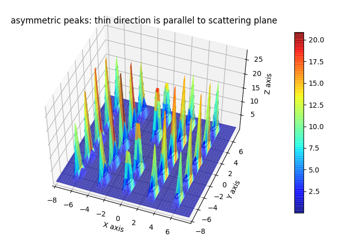
# We orient to 010 direction perpendicular to center of qxy plane
sclattice.rotatehkl2Vector([0, 1, 0], [0, 0, 1])
ffs = js.sf.orientedLatticeStructureFactor(qxyz, sclattice, domainsize=ds, rmsd=0.1, hklmax=2)
fig2 = js.mpl.surface(qxyz[:, 0], qxyz[:, 1], ffs[3].array)
fig2.axes[0].set_title('asymmetric peaks: thin direction is parallel to scattering plane')
fig2.show()

# rhombic lattice simple and body centered

import jscatter as js
import numpy as np

# make xy grid in q space
R = 8  # maximum
N = 50  # number of points
qxy = np.mgrid[-R:R:N * 1j, -R:R:N * 1j].reshape(2, -1).T
# add z=0 component
qxyz = np.c_[qxy, np.zeros(N ** 2)]
# create rhombic  bc lattice which includes reciprocal lattice vectors and methods to get peak positions
rblattice = js.lattice.rhombicLattice([[2, 0, 0], [0, 3, 0], [0, 0, 1]], size=[5, 5, 5],
                                      unitCellAtoms=[[0, 0, 0], [0.5, 0.5, 0.5]])
# We orient to 100 direction perpendicular to xy plane
rblattice.rotatehkl2Vector([1, 0, 0], [0, 0, 1])

# define crystal size in directions
ds = [[20, 1, 0, 0], [5, 0, 1, 0], [5, 0, 0, 1]]
ffs = js.sf.orientedLatticeStructureFactor(qxyz, rblattice, domainsize=ds, rmsd=0.1, hklmax=2)
fig = js.mpl.surface(ffs.X, ffs.Z, ffs[3].array)
fig.axes[0].set_title('rhombic body centered lattice')
fig.show()
# same without body centered atom
tlattice = js.lattice.rhombicLattice([[2, 0, 0], [0, 3, 0], [0, 0, 1]], size=[5, 5, 5])
tlattice.rotatehkl2Vector([1, 0, 0], [0, 0, 1])
ffs = js.sf.orientedLatticeStructureFactor(qxyz, tlattice, domainsize=ds, rmsd=0.1, hklmax=2)
fig2 = js.mpl.surface(ffs.X, ffs.Z, ffs[3].array)
fig2.axes[0].set_title('rhombic lattice')
fig2.show()

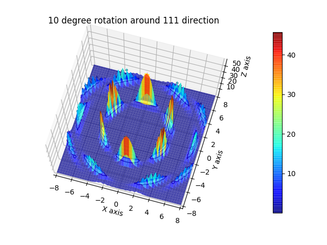
# Rotation of 10 degrees along [1,1,1] axis. It looks spiky because of low number of points in xy plane ::

import jscatter as js
import numpy as np

# make xy grid in q space
R = 8  # maximum
N = 800  # number of points
qxy = np.mgrid[-R:R:N * 1j, -R:R:N * 1j].reshape(2, -1).T
# add z=0 component
qxyz = np.c_[qxy, np.zeros(N ** 2)]  # as position vectors
# create sc lattice which includes reciprocal lattice vectors and methods to get peak positions
sclattice = js.lattice.scLattice(2.1, 5)
# We orient to 111 direction perpendicular to xy plane
sclattice.rotatehkl2Vector([1, 1, 1], [0, 0, 1])
# this needs crystal rotation by 15 degrees to be aligned to xy plane after rotation to 111 direction
# The crystals rotates by 10 degrees around 111 to broaden peaks.
ds = 15
fpi = np.pi / 180.
ffs = js.sf.orientedLatticeStructureFactor(qxyz, sclattice, rotation=[1, 1, 1, 10 * fpi],
                                           domainsize=ds, rmsd=0.1, hklmax=2, nGauss=23)
fig = js.mpl.surface(ffs.X, ffs.Z, ffs[3].array)
fig.axes[0].set_title('10 degree rotation around 111 direction')
fig.show()

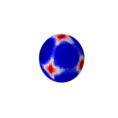
Ewald Sphere of simple cubic lattice

import jscatter as js
import numpy as np

import matplotlib.pyplot as pyplot
from matplotlib import cm

phi, theta = np.meshgrid(np.r_[0:np.pi:45j], np.r_[0:2 * np.pi:90j])

# The Cartesian coordinates of the sphere
q = 3
x = q * (np.sin(phi) * np.cos(theta) + 1)
y = q * np.sin(phi) * np.sin(theta)
z = q * np.cos(phi)
qxzy = np.asarray([x, y, z]).reshape(3, -1).T

sclattice = js.lattice.scLattice(2.1, 5)
ffe = js.ff.orientedCloudScattering(qxzy, sclattice.XYZ, mosaicity=[5,0,0], nCone=20, rms=0.02)

# log scale for colors
ffey = np.log(ffe.Y)
fmax, fmin = ffey.max(), ffey.min()
ffeY = (np.reshape(ffey, x.shape) - fmin) / (fmax - fmin)

# Set the aspect ratio to 1 so our sphere looks spherical
fig = pyplot.figure(figsize=pyplot.figaspect(1.))
ax = fig.add_subplot(111, projection='3d')
ax.plot_surface(x, y, z, rstride=1, cstride=1, facecolors=cm.seismic(ffeY))

# Turn off the axis planes
ax.set_axis_off()
pyplot.show(block=False)

# ------------------------------------

phi, theta = np.meshgrid(np.r_[0:np.pi:90j], np.r_[0:1 * np.pi:90j])
# The Cartesian coordinates of the unit sphere
q = 8
x = q * (np.sin(phi) * np.cos(theta) + 1)
y = q * np.sin(phi) * np.sin(theta)
z = q * np.cos(phi)
qxzy = np.asarray([x, y, z]).reshape(3, -1).T

# Set the aspect ratio to 1 so our sphere looks spherical
fig = pyplot.figure(figsize=pyplot.figaspect(1.))
ax = fig.add_subplot(111, projection='3d')

# create lattice and show it scaled
sclattice = js.lattice.scLattice(2.1, 1)
sclattice.rotatehkl2Vector([1, 1, 1], [0, 0, 1])
gg = ax.scatter(sclattice.X / 3 + q, sclattice.Y / 3, sclattice.Z / 3, c='k', alpha=0.9)
gg.set_visible(True)

ds = 15
fpi = np.pi / 180.
ffs = js.sf.orientedLatticeStructureFactor(qxzy, sclattice, rotation=None, domainsize=ds, rmsd=0.1, hklmax=2, nGauss=23)
# show scattering in log scale on Ewald sphere
ffsy = np.log(ffs.Y)
fmax, fmin = ffsy.max(), ffsy.min()
ffsY = (np.reshape(ffsy, x.shape) - fmin) / (fmax - fmin)

ax.plot_surface(x, y, z, rstride=1, cstride=1, facecolors=cm.hsv(ffsY), alpha=0.4)
ax.plot([q, 2 * q], [0, 0], [0, 0], color='k')
pyplot.show(block=False)

#  ad flat detector xy plane
xzw = np.mgrid[-8:8:80j, -8:8:80j]
qxzw = np.stack([np.zeros_like(xzw[0]), xzw[0], xzw[1]], axis=0)

ff2 = js.sf.orientedLatticeStructureFactor(qxzw.reshape(3, -1).T, sclattice, rotation=None, domainsize=ds, rmsd=0.1,
                                           hklmax=2, nGauss=23)
ffs2 = np.log(ff2.Y)
fmax, fmin = ffs2.max(), ffs2.min()
ff2Y = (np.reshape(ffs2, xzw[0].shape) - fmin) / (fmax - fmin)
ax.plot_surface(qxzw[0], qxzw[1], qxzw[2], rstride=1, cstride=1, facecolors=cm.gist_ncar(ff2Y), alpha=0.3)
ax.set_xlabel('x axis')
ax.set_ylabel('y axis')
ax.set_zlabel('z axis')

fig.suptitle('Scattering plane and Ewald sphere of lattice \nmatplotlib is limited in 3D')
pyplot.show(block=False)
# matplotlib is not real 3D rendering
# maybe use later something else

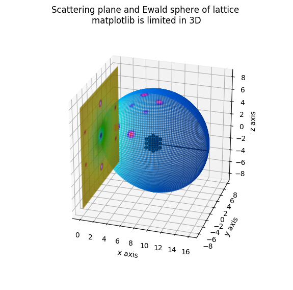
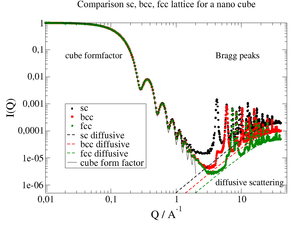
A nano cube build of different lattices

Here we build a nano cube from different crystal structures.

We can observe the cube formfactor and at larger Q the crystal peaks broadened by the small size. The scattering is explicitly calculated from the grids by ff.cloudScattering. Smoothing with a Gaussian considers experimental broadening (and smooth the result:-).

relError is set to higher value to speed it up. For precise calculation decrease it. For the pictures it was 0.02, this takes about 26 s on 6 core CPU for last bcc example with about 10000 atoms and 900 Q values.

Model with explicit atom positions in small grid

The peaks at large Q are Bragg peaks. Due to the small size extinction rules are not fulfilled completely, which is best visible at first peak positions where we still observe forbidden peaks for bcc and fcc. All Bragg peaks are shown in the second example. The formfactor shows reduced amplitudes due to Debye-Waller factor (rms) and the number of grid atoms. The analytical solution has infinite high density of atoms and a sharp interface.

import jscatter as js
import numpy as np

q = np.r_[js.loglist(0.01, 3, 200), 3:40:800j]
unitcelllength = 1.5
N = 8
rms = 0.05
relError = 20  # 0.02 for picture below

# make grids and calc scattering
scgrid = js.sf.scLattice(unitcelllength, N)
sc = js.ff.cloudScattering(q, scgrid.points, relError=relError, rms=rms)
bccgrid = js.sf.bccLattice(unitcelllength, N)
bcc = js.ff.cloudScattering(q, bccgrid.points, relError=relError, rms=rms)
fccgrid = js.sf.fccLattice(unitcelllength, N)
fcc = js.ff.cloudScattering(q, fccgrid.points, relError=relError, rms=rms)
#
# plot  data
p = js.grace(1.5, 1)
# smooth with Gaussian to include instrument resolution
p.plot(sc.X, js.formel.smooth(sc, 10, window='gaussian'), legend='sc')
p.plot(bcc.X, js.formel.smooth(bcc, 10, window='gaussian'), legend='bcc')
p.plot(fcc.X, js.formel.smooth(fcc, 10, window='gaussian'), legend='fcc')
#
# diffusive scattering
# while cloudScattering is normalized to one (without normalization ~ N**2),
# diffusive is proportional to scattering of single atoms (incoherent ~ N)
q = q = js.loglist(1, 35, 100)
p.plot(q, (1 - np.exp(-q * q * rms ** 2)) / scgrid.numberOfAtoms(), li=[3, 2, 1], sy=0, le='sc diffusive')
p.plot(q, (1 - np.exp(-q * q * rms ** 2)) / bccgrid.numberOfAtoms(), li=[3, 2, 2], sy=0, le='bcc diffusive')
p.plot(q, (1 - np.exp(-q * q * rms ** 2)) / fccgrid.numberOfAtoms(), li=[3, 2, 3], sy=0, le='fcc diffusive')
#
# cuboid formfactor for small Q
q = js.loglist(0.01, 2, 300)
cube = js.ff.cuboid(q, unitcelllength * (2 * N + 1))
p.plot(cube.X, js.formel.smooth(cube, 10, window='gaussian') / cube.Y[0], sy=0, li=1, le='cube form factor')
#
p.title('Comparison sc, bcc, fcc lattice for a nano cube')
p.yaxis(scale='l', label='I(Q)', max=1, min=5e-7)
p.xaxis(scale='l', label=r'Q / A\S-1', max=50, min=0.01)
p.legend(x=0.02, y=0.001, charsize=1.5)
p.text('cube formfactor', x=0.02, y=0.05, charsize=1.4)
p.text('Bragg peaks', x=4, y=0.05, charsize=1.4)
p.text('diffusive scattering', x=4, y=1e-6, charsize=1.4)
p.save('LatticeComparison.png')

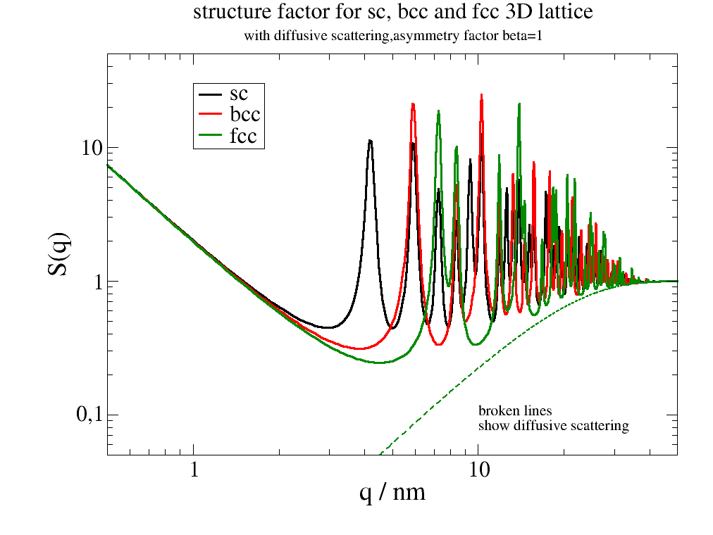
Analytical model assuming crystal lattice with limited size

This shows the Bragg peaks of crystal structures with broadening due to limited size.

The low Q scattering from the chrystal shape is not covered well as only the asymptotic behavior is governed.

import jscatter as js
import numpy as np

q = np.r_[js.loglist(0.5, 3, 50), 3:80:1200j]
unitcelllength = 1.5
N = 8
a = 1.5  # unit cell length
domainsize = a * (2 * N + 1)
rms = 0.05
p = js.grace(1.5, 1)
p.title('structure factor for sc, bcc and fcc 3D lattice')
p.subtitle('with diffusive scattering,asymmetry factor beta=1')

scgrid = js.sf.scLattice(unitcelllength, N)
sc = js.sf.latticeStructureFactor(q, lattice=scgrid, rmsd=rms, domainsize=domainsize)
p.plot(sc, li=[1, 3, 1], sy=0, le='sc')
p.plot(sc.X, 1 - sc[-3], li=[3, 2, 1], sy=0)  # diffusive scattering

bccgrid = js.sf.bccLattice(unitcelllength, N)
bcc = js.sf.latticeStructureFactor(q, lattice=bccgrid, rmsd=rms, domainsize=domainsize)
p.plot(bcc, li=[1, 3, 2], sy=0, le='bcc')
p.plot(bcc.X, 1 - bcc[-3], li=[3, 2, 2], sy=0)

fccgrid = js.sf.fccLattice(unitcelllength, N)
fcc = js.sf.latticeStructureFactor(q, lattice=fccgrid, rmsd=rms, domainsize=domainsize)
p.plot(fcc, li=[1, 3, 3], sy=0, le='fcc')
p.plot(fcc.X, 1 - fcc[-3], li=[3, 2, 3], sy=0)

p.text(r"broken lines \nshow diffusive scattering", x=10, y=0.1)
p.yaxis(label='S(q)', scale='l', max=50, min=0.05)
p.xaxis(label=r'q / A\S-1', scale='l', max=50, min=0.5)
p.legend(x=1, y=30, charsize=1.5)
p.save('LatticeComparison2.png')

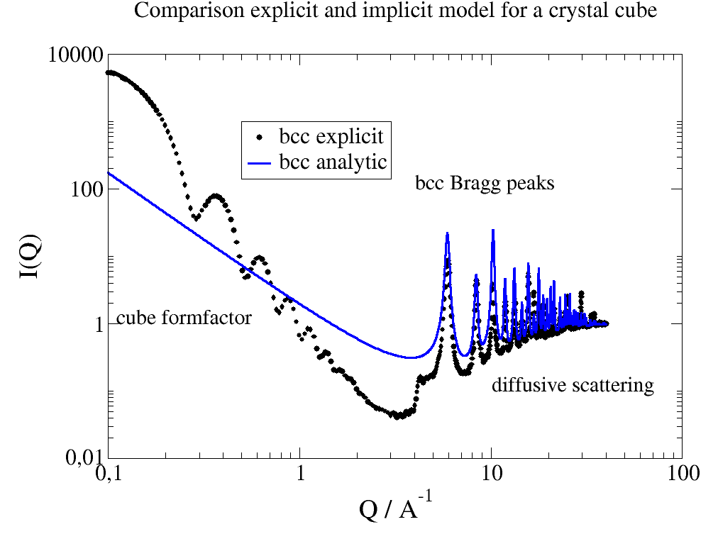
A direct comparison between both models for bcc cube

Differences are due to incomplete extinction of peaks and due to explicit dependence on the edges (incomplete elementary cells)

relError=0.02 samples until the error is smaller 0.02 for a q point with pseudorandom numbers. The same can be done with relError=400 on a fixed Fibonacci lattice. Both need longer for the computation.

The 1/q² power law at low q for the analytic model results from integration over infinite, d=3 dimensional q space. For a real nanoparticle or crystal domain the size (~ integration volume ) is finite resulting in the typical formfactor behavior with a plateau for lowest q, a Guinier range determined by Rg and a Porod region at higher q dependent on the fractal structure.

formfactor behavior with a plateau for lowest q, a Guinier range determined by Rg
and a Porod region at higher q dependent on the fractal structure.  

#end3
"""

import jscatter as js
import numpy as np

q = np.r_[js.loglist(0.1, 3, 100), 3:40:800j]
unitcelllength = 1.5
N = 8
rms = 0.05
relError = 20  # 0.02 for the picture below
domainsize = unitcelllength * (2 * N + 1)

bccgrid = js.sf.bccLattice(unitcelllength, N)
bcc = js.ff.cloudScattering(q, bccgrid.points, relError=relError, rms=rms)
p = js.grace(1.5, 1)
p.plot(bcc.X, js.formel.smooth(bcc, 10, window='gaussian') * bccgrid.numberOfAtoms(), legend='bcc explicit')

q = np.r_[js.loglist(0.1, 3, 200), 3:40:1600j]
sc = js.sf.latticeStructureFactor(q, lattice=bccgrid, rmsd=rms, domainsize=domainsize)
p.plot(sc, li=[1, 3, 4], sy=0, le='bcc analytic')
p.yaxis(scale='l', label='I(Q)', max=20000, min=0.05)
p.xaxis(scale='l', label=r'Q / A\S-1', max=50, min=0.1)
p.legend(x=0.5, y=1000, charsize=1.5)
p.title('Comparison explicit and implicit model for a crystal cube')
p.text('cube formfactor', x=0.11, y=1, charsize=1.4)
p.text('bcc Bragg peaks', x=4, y=100, charsize=1.4)
p.text('diffusive scattering', x=10, y=0.1, charsize=1.4)
p.save('LatticeComparison3.png')

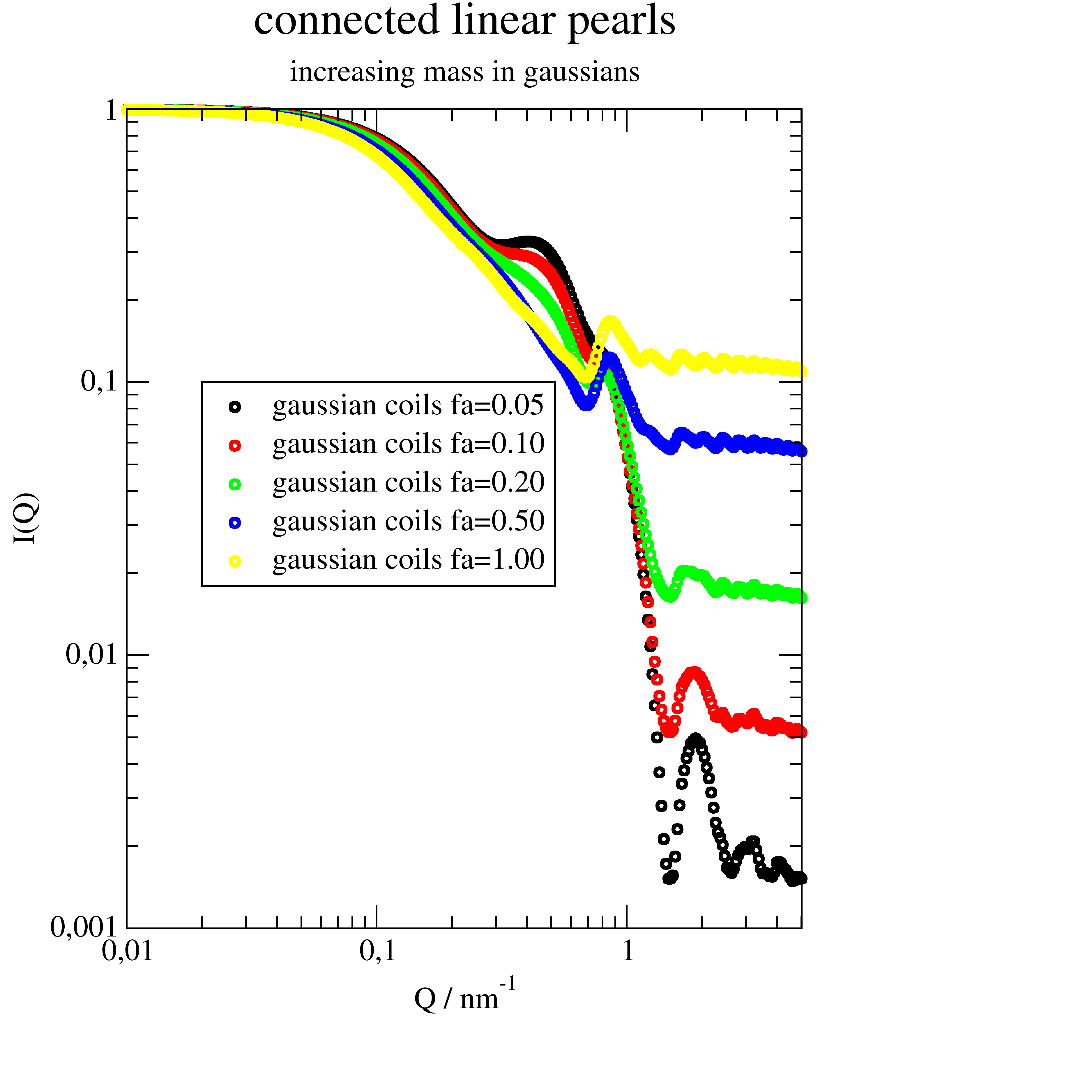
Linear Pearls with connecting coils

The example uses cloudscattering to build a line of spheres. Between the spheres are Gaussian coils to represent chains connecting the spheres. The model linearPearls() is very similar build but uses a simpler build of the linear chain.

import jscatter as js
import numpy as np

q = js.loglist(0.01, 5, 300)

# create array containing formfactors
# columns will be [q, sphere, gaussian chain]
ffs = js.ff.sphere(q[::2], 3)
ffg = js.ff.gaussianChain(q[::2], 0.1)
ff = ffs.addColumn(1, ffg.Y)

# line of points
scl = js.sf.scLattice(8, [2, 0, 0])
# alternating sphere [1] anf gaussian coils [2]
grid1 = np.c_[scl.points, np.r_[[1] * 5]]
grid1[::2, -1] = 2

# grid points have default b=1
# we change gaussians to fa
p = js.grace()
for i, fa in enumerate([0.05, 0.1, 0.2, 0.5, 1], 1):
    grid1[::2, -2] = fa
    fq = js.ff.cloudScattering(q, grid1, relError=0, formfactoramp=ff)
    p.plot(fq, sy=[1, 0.4, i], le='gaussian coils fa={0:.2f}'.format(fa))

p.yaxis(scale='l', label='I(Q)')
p.xaxis(scale='l', label=r'Q / nm\S-1')
p.title('connected linear pearls')
p.subtitle('increasing mass in gaussians')
p.legend(x=0.02, y=0.1)
p.save('connected_linearPearls.png', size=(3, 3), dpi=150)

# same with orientation in 2D
grid1[::2, -2] = 0.1
qxzw = np.mgrid[-6:6:50j, -6:6:50j].reshape(2, -1).T
ffe = js.ff.orientedCloudScattering(qxzw, grid1, mosaicity=[5,0,0], nCone=10, rms=0)
fig = js.mpl.surface(ffe.X, ffe.Z, ffe.Y)
fig.axes[0].set_title(r'cos**2 for Z and slow decay for X due to 5 degree cone')
fig.show()